
Homogeneity of Variance, Equal Variances, ANOVA Assumption and Group Spread
Bartlett’s Test: Formula, Interpretation, SPSS, Python, R and Excel Guide
Bartlett’s Test is a statistical test used to check whether two or more independent groups have equal variances. It is commonly used before ANOVA or other group-comparison methods when the equal variance assumption matters. This Salar Cafe guide explains Bartlett’s Test with verified SPSS output, Python charts, R validation charts, formulas, null and alternative hypotheses, group variance interpretation, p-value decision, Excel workflow, SPSS syntax, Python code, R code, APA reporting, common mistakes and downloadable resources.
Google AdSense top placement reserved here
Quick Answer: Bartlett’s Test Result
The verified SPSS output compares the variance of G3 final grade across the two sex groups, F and M. The female group has N = 383, mean = 12.25, standard deviation = 3.124, and variance = 9.760. The male group has N = 266, mean = 11.41, standard deviation = 3.321, and variance = 11.027. The total sample has N = 649, mean = 11.91, standard deviation = 3.231, and variance = 10.437.
The Bartlett’s Test result reports k = 2 groups, total N = 649, pooled variance = 10.27911, Bartlett chi-square = 1.17082, df = 1, and p = .27923. Since the p-value is greater than .05, we fail to reject the null hypothesis. This means the evidence is not strong enough to conclude that the group variances are significantly different.
Hypothesis-style interpretation: The null hypothesis says the group variances are equal. The alternative hypothesis says at least one group variance is different. Since p = .27923, the test does not find a statistically significant variance difference between the female and male G3 final grade groups. For this output, Bartlett’s Test supports the equal variance assumption.
Final interpretation: Bartlett’s Test is not significant, χ²(1) = 1.17082, p = .27923. Therefore, the G3 final grade variances for female and male students are not significantly different at the .05 level. The equal variance assumption is acceptable according to Bartlett’s Test.
Important note: Bartlett’s Test is sensitive to non-normality. The SPSS normality context shows that both sex groups have significant normality tests for G3: female group Kolmogorov-Smirnov = .105, p < .001; Shapiro-Wilk = .934, p < .001, and male group Kolmogorov-Smirnov = .148, p < .001; Shapiro-Wilk = .913, p < .001. Because of this, it is wise to compare Bartlett’s Test with robust alternatives such as Levene’s test and the Brown-Forsythe test.
Table of Contents
- What Is Bartlett’s Test?
- Why Bartlett’s Test Matters
- Bartlett’s Test Formula
- Null and Alternative Hypothesis
- Dataset and Variables Used
- Verified SPSS Output Interpretation
- Python Chart-by-Chart Interpretation
- R Chart-by-Chart Validation
- SPSS, R, Python and Excel Workflows
- Code Blocks for Bartlett’s Test
- APA Reporting Wording
- Common Mistakes
- When to Use Bartlett’s Test
- Downloads and Resources
- Related Guides
- FAQs
What Is Bartlett’s Test?
Bartlett’s Test is a homogeneity-of-variance test. It checks whether the variances of a numeric variable are equal across two or more independent groups. In this guide, the numeric variable is G3 final grade, and the grouping variable is sex, with the groups F and M.
The test is commonly used when analysts need to decide whether the equal variance assumption is reasonable before running an analysis that relies on similar group variances. For example, a one-way ANOVA assumes that the dependent variable has roughly equal variances across groups. Bartlett’s Test gives a formal statistical decision about this assumption.
The key idea is simple: if group variances are similar, the test statistic is small and the p-value is usually not significant. If group variances are very different, the test statistic becomes larger and the p-value becomes smaller. In this example, the female variance is 9.760 and the male variance is 11.027. These values are close enough that Bartlett’s Test gives p = .27923, so the equal variance assumption is not rejected.
Bartlett’s Test is strongly connected with other variance and assumption checks. If the data are clearly non-normal, compare its conclusion with Levene’s test, Brown-Forsythe test, Cochran’s C test, and Goldfeld-Quandt test. If you are checking distribution shape before choosing Bartlett’s Test, review the Q-Q plot normality check, P-P plot normality check, Kolmogorov-Smirnov test, Lilliefors test, D’Agostino-Pearson test, and Cramer-von Mises test.
Practical meaning: Bartlett’s Test answers this question: “Are the group variances similar enough that the equal variance assumption is reasonable?” In this example, the answer is yes according to Bartlett’s Test, because p = .27923.
Why Bartlett’s Test Matters
Bartlett’s Test matters because many group-comparison methods are affected by unequal variances. When one group has much larger spread than another, standard tests can produce misleading p-values, confidence intervals and conclusions. Checking variance equality helps you decide whether the ordinary equal-variance method is acceptable or whether a robust alternative is needed.
In the verified SPSS output, the female group has a standard deviation of 3.124, while the male group has a standard deviation of 3.321. The male group is slightly more variable, but the difference is not statistically significant under Bartlett’s Test. Therefore, for this specific comparison of G3 by sex, there is no strong evidence of unequal variances.
| Reason to Use Bartlett’s Test | What It Checks | Why It Helps |
|---|---|---|
| ANOVA assumption checking | Whether group variances are equal. | Supports the decision to use ordinary ANOVA when assumptions are acceptable. |
| Group spread comparison | Whether one group has much larger spread than another. | Prevents misleading interpretation of group differences. |
| Pre-test diagnostic workflow | Whether variance assumptions are reasonable before hypothesis testing. | Helps choose between ordinary and robust methods. |
| Reporting transparency | Whether the equal variance assumption was tested and documented. | Improves thesis, dissertation, research and consulting reports. |
| Software validation | Whether SPSS, Python and R support the same decision. | Strengthens reproducibility and confidence in the result. |
For a complete reporting workflow, Bartlett’s Test should be supported by descriptive summaries, boxplots and standard deviation comparisons. Use descriptive statistics, frequency distribution, histogram interpretation, box plot interpretation, five-number summary, and coefficient of variation to explain the group spread before reporting the formal test.
Bartlett’s Test Formula
Bartlett’s Test compares the natural logarithm of the pooled variance with the weighted natural logarithms of the group variances. The test statistic is approximately chi-square distributed when the normality assumption is reasonable.
Let k be the number of groups, ni be the sample size of group i, si2 be the variance of group i, and N be the total sample size.
1. Pooled Variance
In the verified SPSS output, the pooled variance is:
2. Bartlett’s Test Statistic
The correction factor is:
3. Degrees of Freedom
For this example, k = 2, so df = 1. The verified result is:
Formula caution: Bartlett’s Test assumes approximate normality inside groups. When group distributions are strongly non-normal, Bartlett’s Test can become too sensitive. In such cases, compare it with Levene’s test or Brown-Forsythe test.
Null and Alternative Hypothesis for Bartlett’s Test
Bartlett’s Test is a formal hypothesis test for equality of variances across groups. In this post, it compares the variance of G3 final grade across the female and male groups.
| Hypothesis | Statement | Meaning in This Example |
|---|---|---|
| Null hypothesis | H0: σF2 = σM2 | The G3 variance is equal for female and male students. |
| Alternative hypothesis | H1: At least one group variance is different. | The G3 variance differs between female and male students. |
| Decision rule | Reject H0 if p < .05. | If p is below .05, equal variances are rejected. |
| Observed result | χ²(1) = 1.17082, p = .27923. | The p-value is greater than .05. |
Hypothesis decision: Because p = .27923 is greater than .05, fail to reject the null hypothesis. The G3 final grade variances are not significantly different between the female and male groups according to Bartlett’s Test.
Interpretation nuance: “Fail to reject equal variances” does not prove the variances are exactly identical. It means the sample does not provide enough evidence to conclude that the group variances differ significantly.
Dataset and Variables Used
The worked example uses a student performance-style dataset. The dependent or measured variable is G3 final grade, and the grouping variable is sex. Bartlett’s Test checks whether the spread of G3 is statistically similar for female and male students.
| Variable | Role | Verified Value / Use | Why It Matters |
|---|---|---|---|
| G3 | Tested numeric variable | Total N = 649, mean = 11.91, SD = 3.231, variance = 10.437 | Final grade variable whose group variances are compared. |
| sex | Grouping variable | Groups: F and M | Defines the independent groups for Bartlett’s Test. |
| Female group | Group 1 | N = 383, mean = 12.25, SD = 3.124, variance = 9.760 | Provides the first group variance. |
| Male group | Group 2 | N = 266, mean = 11.41, SD = 3.321, variance = 11.027 | Provides the second group variance. |
| Pooled variance | Bartlett calculation component | 10.27911 | Weighted estimate of common variance under the equal-variance null hypothesis. |
Before applying Bartlett’s Test, always inspect the group distributions. In this example, the normality context is important because the SPSS normality tests are significant in both groups. Use normality and shape guides such as Q-Q plot normality check, P-P plot normality check, histogram interpretation, and box plot interpretation before relying only on the Bartlett p-value.
Google AdSense middle placement reserved here
Verified SPSS Output Interpretation
The verified SPSS output provides the group descriptives, normality context, Bartlett variance components and final equal-variance decision. The output compares G3 final grade by sex. There are 649 included cases, 0 excluded cases, and 649 total cases.
The SPSS output PDF for this guide is available here:
Download SPSS Bartlett’s Test Output PDF
Verified SPSS output for Bartlett’s Test, group descriptives, normality context and equal-variance decision.
Copy SPSS, Python, R and Excel Code
Use the code section below to reproduce the Bartlett’s Test workflow.
SPSS Group Descriptives
| Group | N | Mean | Standard Deviation | Variance | Interpretation |
|---|---|---|---|---|---|
| Female | 383 | 12.25 | 3.124 | 9.760 | The female group has slightly lower spread than the male group. |
| Male | 266 | 11.41 | 3.321 | 11.027 | The male group has slightly higher spread, but not enough to be significant in Bartlett’s Test. |
| Total | 649 | 11.91 | 3.231 | 10.437 | The total spread summarizes both groups together. |
SPSS Normality Context
| Group | Kolmogorov-Smirnov | Shapiro-Wilk | Normality Interpretation |
|---|---|---|---|
| Female | Statistic = .105, df = 383, p < .001 | W = .934, df = 383, p < .001 | Normality is rejected for the female G3 distribution. |
| Male | Statistic = .148, df = 266, p < .001 | W = .913, df = 266, p < .001 | Normality is rejected for the male G3 distribution. |
SPSS Bartlett’s Test Result
| Output Item | Verified Result | Interpretation |
|---|---|---|
| Number of groups | 2 | Female and male groups were compared. |
| Total N | 649 | All valid cases were included. |
| Pooled variance | 10.27911 | Weighted estimate of common variance under equal variance assumption. |
| Bartlett chi-square | 1.17082 | The test statistic is small relative to the chi-square reference distribution. |
| Degrees of freedom | 1 | df = k − 1 = 2 − 1. |
| p-value | .27923 | The p-value is greater than .05. |
| Reject equal variances at .05? | No | Fail to reject the equal variance assumption. |
SPSS Decision Summary
SPSS interpretation summary: Bartlett’s Test for G3 across sex groups produced χ²(1) = 1.17082 with p = .27923. Since the p-value is greater than .05, the test does not reject the equality of variances. The female variance was 9.760 and the male variance was 11.027, but this difference was not statistically significant.
How to Handle the Normality Warning
The normality context shows significant normality tests in both groups. Because Bartlett’s Test is sensitive to non-normality, the safest reporting strategy is to state both findings: Bartlett’s Test did not find unequal variances, but because group distributions departed from normality, a robust variance test such as Levene’s test or Brown-Forsythe test should also be considered. This balanced interpretation is stronger than reporting Bartlett’s p-value alone.
Python Chart-by-Chart Interpretation
The Python charts show Bartlett’s Test visually. They explain group spread, group variance comparison, p-value decision, normality context and group size with standard deviation. These visuals help turn the variance test into a clear report.
Python Chart 1: Group Spread Boxplots
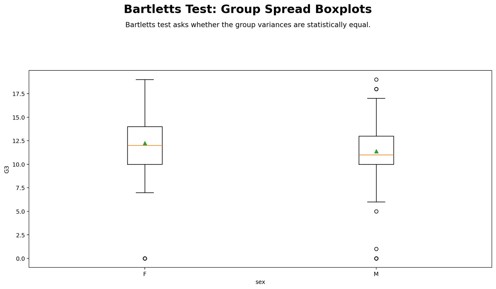
This chart shows the distribution of G3 final grades by group. Boxplots are useful before Bartlett’s Test because they show the median, interquartile range, overall spread and possible unusual values. If one group’s box or whiskers were much wider than the other group’s, that would visually suggest unequal variance.
In this example, the female and male spreads are broadly similar. The male group has a slightly larger standard deviation and variance, but the difference is not visually extreme. This matches the SPSS result where the female variance is 9.760 and the male variance is 11.027.
Decision/reporting conclusion: The boxplots support the Bartlett’s Test decision. The group spreads do not appear dramatically different, and the formal test does not reject equal variances.
Python Chart 2: Group Variance Comparison
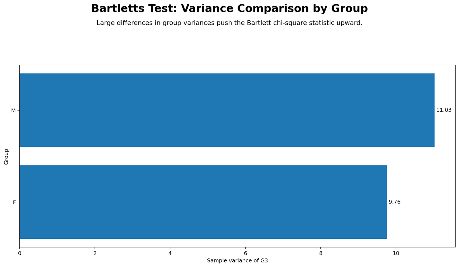
This chart directly compares the variance values used in Bartlett’s Test. The female group variance is 9.760, and the male group variance is 11.027. The male variance is numerically higher, but the difference is modest.
Bartlett’s Test evaluates whether this observed variance difference is large enough to be statistically significant. The result, χ²(1) = 1.17082, p = .27923, shows that the difference is not statistically significant at the .05 level.
Decision/reporting conclusion: Report that the variance comparison chart shows only a modest variance difference, and Bartlett’s Test confirms that the difference is not statistically significant.
Python Chart 3: Bartlett p-value Decision
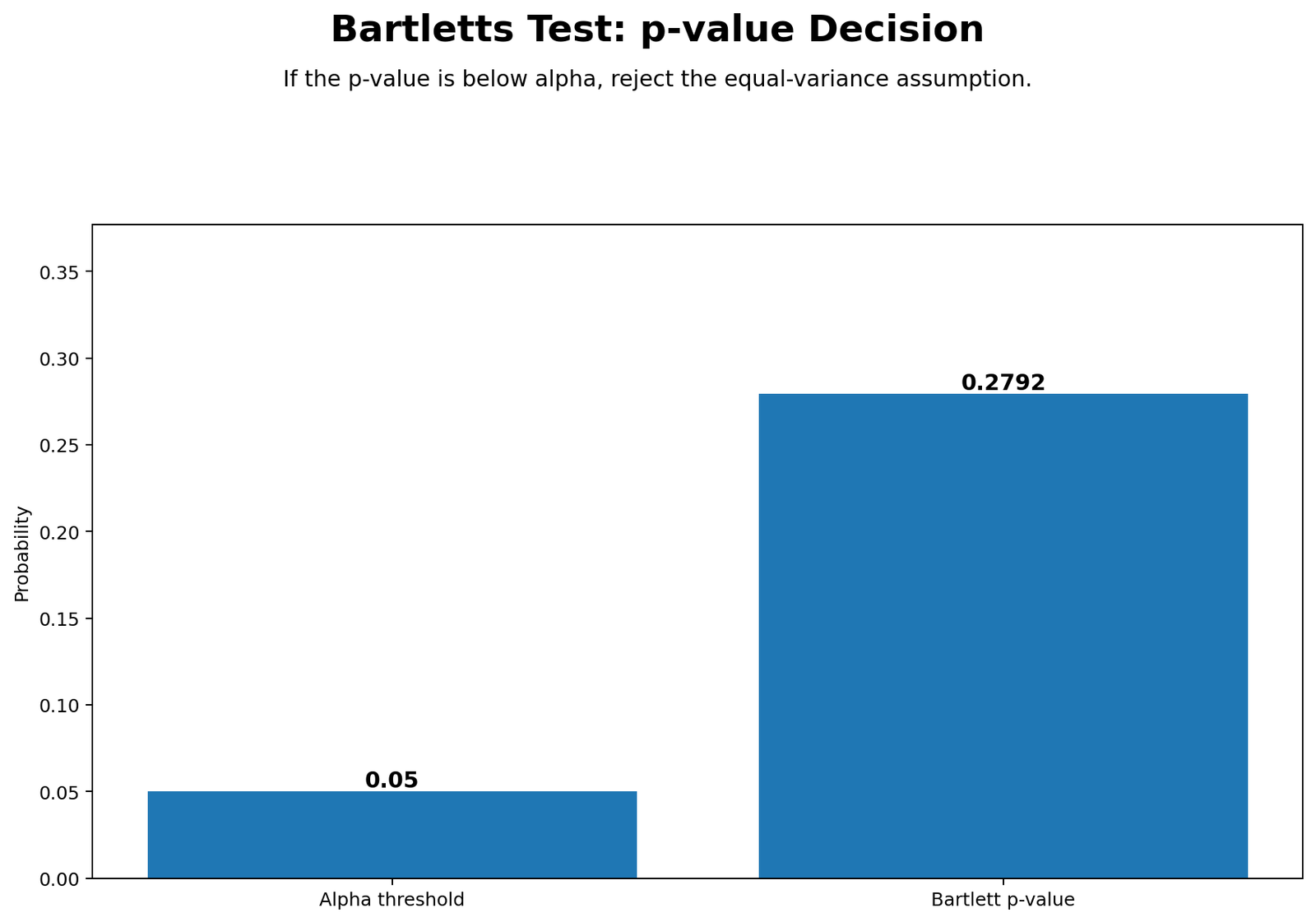
This chart presents the most important decision visually. Bartlett’s Test gives a p-value of .27923. Since this value is greater than the common alpha level of .05, the correct decision is to fail to reject the null hypothesis of equal variances.
A p-value chart is useful for student reports because it makes the decision rule obvious. The p-value sits above the rejection boundary, so the test does not provide evidence that the group variances are different.
Decision/reporting conclusion: Report that Bartlett’s Test was not statistically significant, p = .27923. The equal variance assumption is acceptable according to Bartlett’s Test.
Python Chart 4: Normality Context Distribution
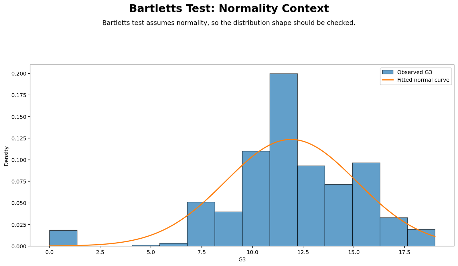
This chart is important because Bartlett’s Test assumes that the group distributions are approximately normal. The SPSS normality context shows that both groups reject normality: female group Shapiro-Wilk W = .934, p < .001, and male group Shapiro-Wilk W = .913, p < .001.
Because of this, the Bartlett result should be interpreted carefully. The non-significant Bartlett result still suggests no strong variance difference, but robust tests are recommended as a confirmation. This is where Levene’s test and Brown-Forsythe test become useful.
Decision/reporting conclusion: Report that the normality context warns against relying only on Bartlett’s Test. The result is non-significant, but robust variance tests should be considered because group normality is not supported.
Python Chart 5: Group Size and Standard Deviation
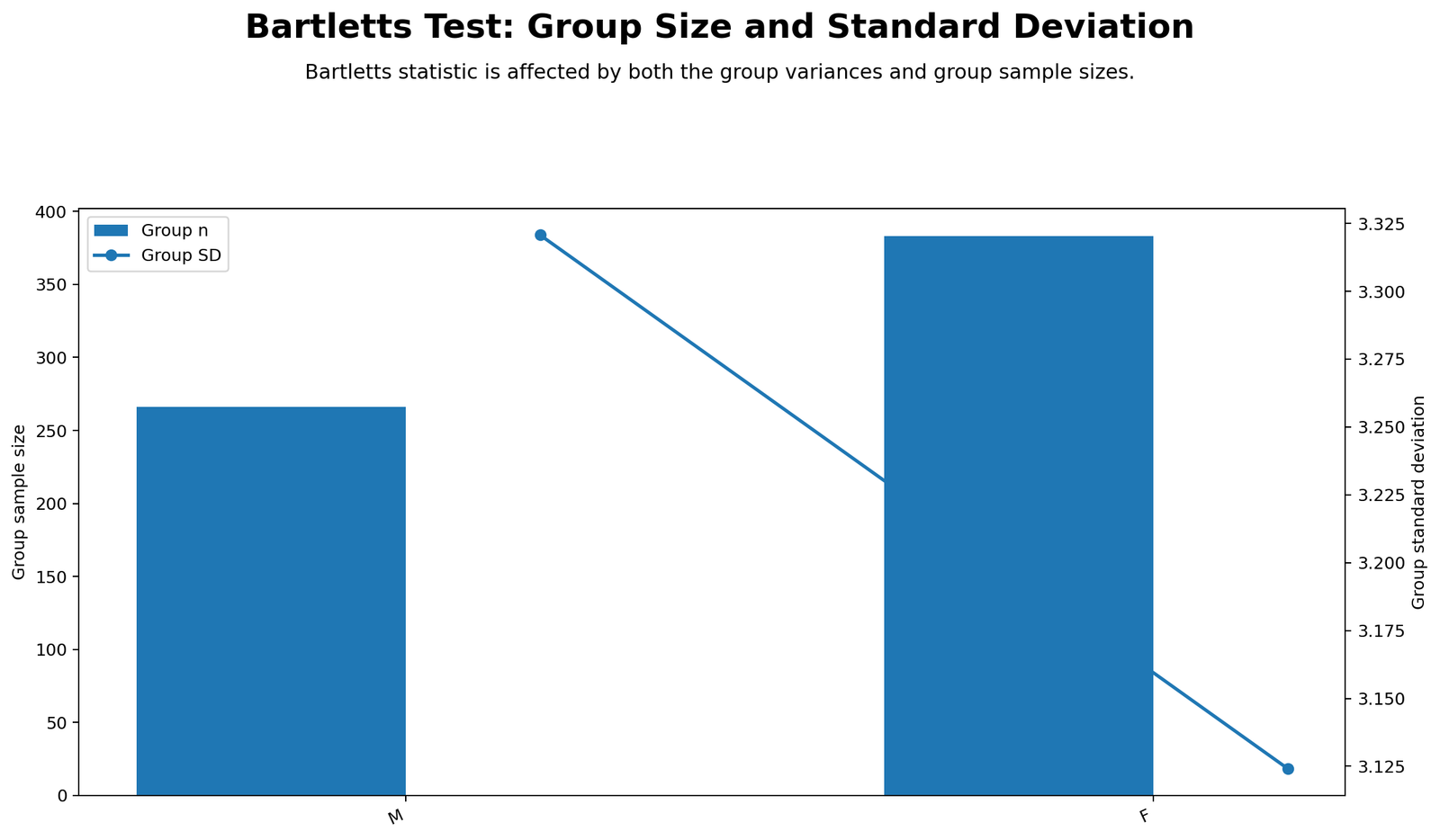
This chart combines group size and spread. The female group has N = 383 and SD = 3.124, while the male group has N = 266 and SD = 3.321. The group sizes are not identical, but both groups are large enough for stable descriptive summaries.
The standard deviations are close, which supports the non-significant Bartlett result. If the standard deviations were very different, the p-value decision might be different, especially with large sample sizes.
Decision/reporting conclusion: Report that the group standard deviations are similar and support the equal variance conclusion. The male group is slightly more variable, but not significantly so under Bartlett’s Test.
R Chart-by-Chart Validation
The R charts validate the same Bartlett’s Test workflow using a separate statistical environment. Agreement between SPSS, Python and R strengthens the conclusion that the group variances are not significantly different.
R Chart 1: Group Spread Boxplots
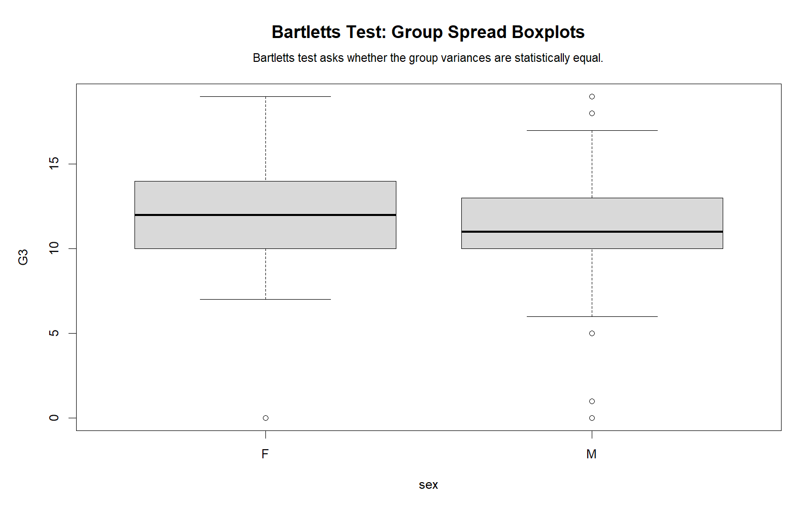
The R boxplot chart validates the Python boxplot interpretation. It shows that the female and male distributions have broadly comparable spread. Any difference in spread appears modest rather than extreme.
Decision/reporting conclusion: Report that the R boxplots confirm the Python visual conclusion: the two groups do not show a large visual variance difference.
R Chart 2: Group Variance Comparison
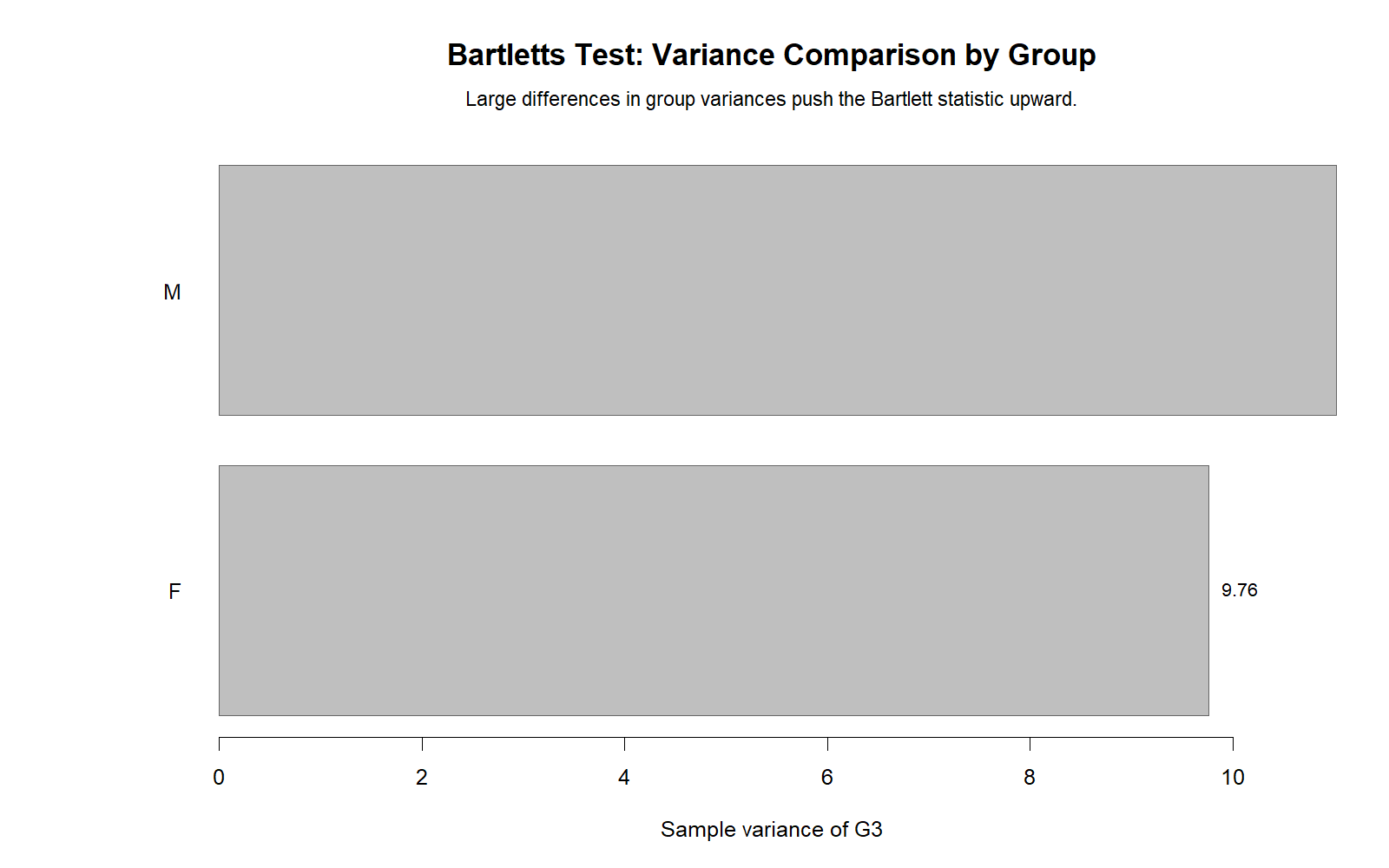
The R variance comparison chart confirms that the male group variance is slightly larger than the female group variance, but the difference is not large enough to reject equal variances. This visual result aligns with χ²(1) = 1.17082, p = .27923.
Decision/reporting conclusion: Report that R validates the same modest variance difference seen in Python and SPSS. The equal variance assumption is not rejected.
R Chart 3: Bartlett p-value Decision
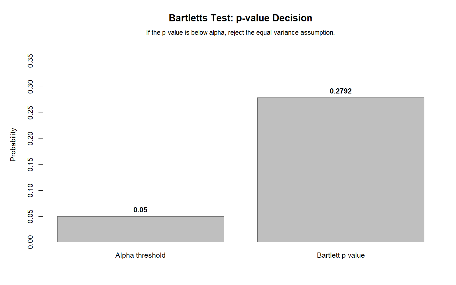
The R p-value decision chart confirms the formal Bartlett conclusion. Because p = .27923 is greater than .05, the test result is not statistically significant. The null hypothesis of equal variances is not rejected.
Decision/reporting conclusion: Report that the R decision chart validates the Python and SPSS decision. Bartlett’s Test supports equal variances for G3 across sex groups.
R Chart 4: Normality Context Distribution
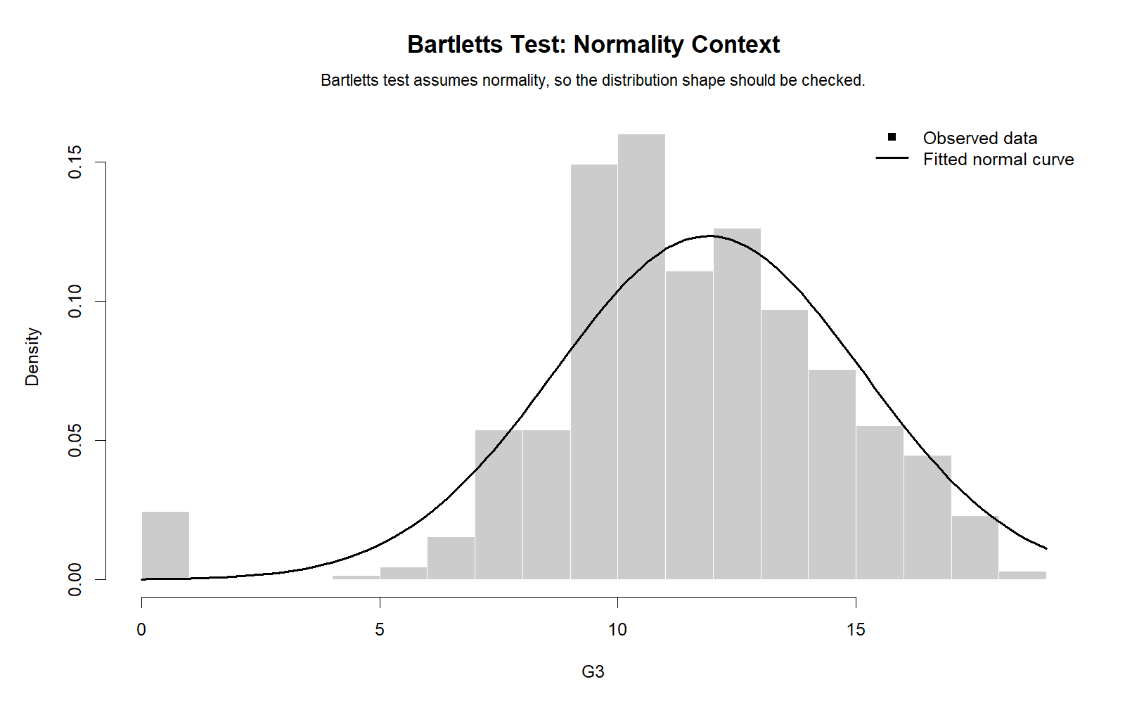
The R normality context chart confirms that Bartlett’s Test should be interpreted with caution when group distributions deviate from normality. The SPSS normality tests are significant in both groups, so the result should be complemented with more robust variance checks.
Decision/reporting conclusion: Report that the R normality context supports the same caution as Python and SPSS. Bartlett’s Test is non-significant, but Levene or Brown-Forsythe can be reported as robustness checks when distributions are non-normal.
R Chart 5: Group Size and Standard Deviation
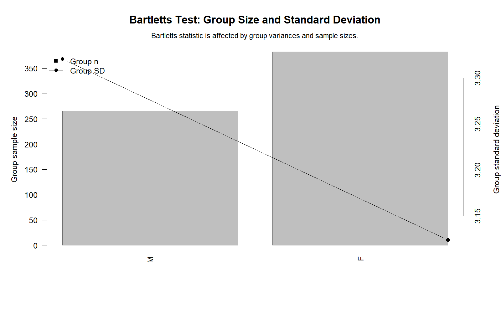
The R group size and standard deviation chart validates the descriptive basis of the test. The female group is larger, but both groups have substantial sample sizes. The standard deviations are close: 3.124 for female students and 3.321 for male students.
Decision/reporting conclusion: Report that R confirms the descriptive similarity in group spread. The standard deviation difference is small and consistent with the non-significant Bartlett result.
Google AdSense in-content placement reserved here
SPSS, R, Python and Excel Workflows for Bartlett’s Test
The Bartlett’s Test workflow is simple across statistical software. First, identify the numeric dependent variable and the independent grouping variable. Second, inspect group descriptive statistics and distribution shape. Third, run Bartlett’s Test. Fourth, interpret the chi-square statistic, degrees of freedom and p-value. Finally, report whether the equal variance assumption is acceptable.
SPSS Workflow
| Step | SPSS Menu or Syntax | Purpose |
|---|---|---|
| Open dataset | File > Open > Data | Load the SPSS-ready dataset. |
| Inspect group descriptives | Analyze > Compare Means > Means | Get N, mean, standard deviation and variance by group. |
| Inspect normality context | Analyze > Descriptive Statistics > Explore | Check histograms, Q-Q plots and normality tests by group. |
| Run Bartlett calculation | SPSS syntax or prepared calculation table | Calculate pooled variance, chi-square statistic, df and p-value. |
| Compare robust tests | Use Levene / Brown-Forsythe where appropriate | Check robustness when normality is questionable. |
| Export output | OUTPUT EXPORT | Save SPSS output PDF for reporting. |
Python Workflow
| Step | Python Action | Purpose |
|---|---|---|
| Read data | pandas.read_csv() | Load the dataset into a DataFrame. |
| Select groups | df.groupby("sex") | Separate G3 values by female and male groups. |
| Calculate descriptives | mean(), std(), var() | Summarize group spread. |
| Run Bartlett’s Test | scipy.stats.bartlett() | Obtain Bartlett statistic and p-value. |
| Create charts | matplotlib | Generate boxplots, variance comparison and p-value decision charts. |
| Report result | APA wording | State whether equal variances are rejected or not rejected. |
R Workflow
| Step | R Action | Purpose |
|---|---|---|
| Read data | read.csv() | Load the dataset. |
| Prepare grouping variable | as.factor() | Ensure the grouping variable is treated as categorical. |
| Run Bartlett’s Test | bartlett.test(G3 ~ sex, data = df) | Calculate Bartlett’s K-squared statistic and p-value. |
| Calculate group summaries | aggregate() or dplyr | Summarize N, SD and variance by group. |
| Create validation charts | ggplot2 | Build R charts to validate the Python and SPSS interpretation. |
Excel Workflow
| Excel Task | Formula or Tool | Purpose |
|---|---|---|
| Separate groups | Filter or create group columns | Place female and male G3 scores in separate columns. |
| Group sample size | =COUNT(range) | Calculate N for each group. |
| Group variance | =VAR.S(range) | Calculate each group variance. |
| Pooled variance | Weighted variance formula | Calculate common variance under H0. |
| Chi-square p-value | =CHISQ.DIST.RT(statistic,df) | Convert Bartlett statistic into p-value. |
Code Blocks for Bartlett’s Test
SPSS Syntax for Bartlett’s Test Support
* Bartlett's Test support in SPSS.
* Example: G3 final grade by sex group.
TITLE "Bartlett's Test: Homogeneity of Variance for G3 by Sex".
DATASET ACTIVATE DataSet1.
* Group descriptives.
MEANS TABLES=G3 BY sex
/CELLS=COUNT MEAN STDDEV VARIANCE.
* Normality context by group.
EXAMINE VARIABLES=G3 BY sex
/PLOT BOXPLOT HISTOGRAM NPPLOT
/COMPARE GROUPS
/STATISTICS DESCRIPTIVES
/CINTERVAL 95
/MISSING LISTWISE
/NOTOTAL.
* If Bartlett components are already calculated in a grouped table,
* report the verified result:
* k = 2, total N = 649, pooled variance = 10.27911,
* Bartlett chi-square = 1.17082, df = 1, p = .27923.
* Robust context: Levene-style test is available through ONEWAY
* when the grouping variable is numeric or properly recoded.
* Example after recoding sex to numeric group:
* ONEWAY G3 BY sex_num
* /STATISTICS HOMOGENEITY
* /MISSING ANALYSIS.
OUTPUT EXPORT
/CONTENTS EXPORT=VISIBLE
/PDF DOCUMENTFILE="Bartletts-Test-SPSS-Output.pdf".Python Code for Bartlett’s Test
import pandas as pd
import numpy as np
from scipy import stats
import matplotlib.pyplot as plt
# Load data
df = pd.read_csv("dataset.csv")
# Prepare variables
df["G3"] = pd.to_numeric(df["G3"], errors="coerce")
df = df.dropna(subset=["G3", "sex"])
# Split groups
groups = [g["G3"].values for name, g in df.groupby("sex")]
group_names = list(df.groupby("sex").groups.keys())
# Group summaries
summary = df.groupby("sex")["G3"].agg(["count", "mean", "std", "var"])
print(summary)
# Bartlett's Test
bart_stat, bart_p = stats.bartlett(*groups)
print("Bartlett chi-square:", bart_stat)
print("Bartlett p-value:", bart_p)
# Decision
alpha = 0.05
if bart_p < alpha:
print("Reject H0: group variances are significantly different.")
else:
print("Fail to reject H0: no significant evidence of unequal variances.")
# Chart 1: Group spread boxplots
plt.figure(figsize=(8, 6))
plt.boxplot(groups, labels=group_names)
plt.xlabel("Group")
plt.ylabel("G3 final grade")
plt.title("Group Spread Boxplots for Bartlett's Test")
plt.tight_layout()
plt.savefig("bartlett-s-test-python-01-chart_01_group_spread_boxplots.png", dpi=300)
plt.close()
# Chart 2: Group variance comparison
plt.figure(figsize=(8, 6))
plt.bar(summary.index.astype(str), summary["var"])
plt.xlabel("Group")
plt.ylabel("Variance")
plt.title("Group Variance Comparison")
plt.tight_layout()
plt.savefig("bartlett-s-test-python-02-chart_02_group_variance_comparison.png", dpi=300)
plt.close()
# Chart 3: Bartlett p-value decision
plt.figure(figsize=(8, 5))
plt.bar(["Bartlett p-value"], [bart_p])
plt.axhline(alpha, linestyle="--")
plt.ylabel("p-value")
plt.title("Bartlett p-value Decision")
plt.tight_layout()
plt.savefig("bartlett-s-test-python-03-chart_03_bartlett_p_value_decision.png", dpi=300)
plt.close()
# Chart 4: Normality context distribution
plt.figure(figsize=(8, 6))
for name, g in df.groupby("sex"):
plt.hist(g["G3"], bins=15, alpha=0.5, label=str(name), density=True)
plt.xlabel("G3 final grade")
plt.ylabel("Density")
plt.title("Normality Context Distribution")
plt.legend()
plt.tight_layout()
plt.savefig("bartlett-s-test-python-04-chart_04_normality_context_distribution.png", dpi=300)
plt.close()
# Chart 5: Group size and standard deviation
fig, ax1 = plt.subplots(figsize=(8, 6))
ax1.bar(summary.index.astype(str), summary["count"], alpha=0.7)
ax1.set_xlabel("Group")
ax1.set_ylabel("Sample size")
ax2 = ax1.twinx()
ax2.plot(summary.index.astype(str), summary["std"], marker="o")
ax2.set_ylabel("Standard deviation")
plt.title("Group Size and Standard Deviation")
fig.tight_layout()
plt.savefig("bartlett-s-test-python-05-chart_05_group_size_and_standard_deviation.png", dpi=300)
plt.close()R Code for Bartlett’s Test
# Bartlett's Test in R
library(ggplot2)
library(dplyr)
df <- read.csv("dataset.csv")
df$G3 <- as.numeric(df$G3)
df$sex <- as.factor(df$sex)
df_clean <- df %>%
filter(!is.na(G3), !is.na(sex))
# Group summaries
summary_table <- df_clean %>%
group_by(sex) %>%
summarise(
n = n(),
mean = mean(G3),
sd = sd(G3),
variance = var(G3),
.groups = "drop"
)
print(summary_table)
# Bartlett's Test
bart_result <- bartlett.test(G3 ~ sex, data = df_clean)
print(bart_result)
# Decision
alpha <- 0.05
if (bart_result$p.value < alpha) {
cat("Reject H0: group variances are significantly different.\n")
} else {
cat("Fail to reject H0: no significant evidence of unequal variances.\n")
}
# Chart 1: Group spread boxplots
ggplot(df_clean, aes(x = sex, y = G3)) +
geom_boxplot() +
labs(title = "Group Spread Boxplots for Bartlett's Test",
x = "Group", y = "G3 final grade")
# Chart 2: Group variance comparison
ggplot(summary_table, aes(x = sex, y = variance)) +
geom_col() +
labs(title = "Group Variance Comparison",
x = "Group", y = "Variance")
# Chart 3: Bartlett p-value decision
p_df <- data.frame(test = "Bartlett p-value", p_value = bart_result$p.value)
ggplot(p_df, aes(x = test, y = p_value)) +
geom_col() +
geom_hline(yintercept = alpha, linetype = "dashed") +
labs(title = "Bartlett p-value Decision",
x = "", y = "p-value")
# Chart 4: Normality context distribution
ggplot(df_clean, aes(x = G3, fill = sex)) +
geom_histogram(aes(y = after_stat(density)), bins = 15, alpha = 0.5, position = "identity") +
labs(title = "Normality Context Distribution",
x = "G3 final grade", y = "Density")
# Chart 5: Group size and standard deviation
ggplot(summary_table, aes(x = sex)) +
geom_col(aes(y = n)) +
geom_point(aes(y = sd * max(n) / max(sd)), size = 3) +
geom_line(aes(y = sd * max(n) / max(sd), group = 1)) +
labs(title = "Group Size and Standard Deviation",
x = "Group", y = "Sample size with scaled SD overlay")Excel Formulas for Bartlett’s Test
Assume:
Female G3 values are in A2:A384.
Male G3 values are in B2:B267.
Female sample size:
=COUNT(A2:A384)
Male sample size:
=COUNT(B2:B267)
Female variance:
=VAR.S(A2:A384)
Male variance:
=VAR.S(B2:B267)
Total N:
=COUNT(A2:A384)+COUNT(B2:B267)
Number of groups:
=2
Pooled variance:
=((n1-1)*var1+(n2-1)*var2)/(N-k)
Correction factor:
=1+(1/(3*(k-1)))*((1/(n1-1)+1/(n2-1))-(1/(N-k)))
Bartlett chi-square:
=(((N-k)*LN(pooled_variance))-((n1-1)*LN(var1)+(n2-1)*LN(var2)))/correction_factor
Degrees of freedom:
=k-1
p-value:
=CHISQ.DIST.RT(bartlett_chisq,df)
Decision:
If p < .05, reject equal variances.
If p >= .05, fail to reject equal variances.APA Reporting Wording for Bartlett’s Test
When reporting Bartlett’s Test, include the tested variable, grouping variable, group variances, test statistic, degrees of freedom, p-value and final equal-variance decision. Also mention the normality context if the group distributions are non-normal.
APA-Style Report
Bartlett’s Test was conducted to evaluate the homogeneity of variance assumption for G3 final grades across sex groups. The female group had a variance of 9.760, and the male group had a variance of 11.027. Bartlett’s Test was not statistically significant, χ²(1) = 1.17082, p = .27923. Therefore, the null hypothesis of equal variances was not rejected, indicating no statistically significant evidence of unequal G3 variances across the two sex groups.
Short Report Sentence
Bartlett’s Test indicated that the G3 variances for female and male students were not significantly different, χ²(1) = 1.17082, p = .27923. Therefore, the equal variance assumption was retained for this comparison.
Normality-Cautious Report Sentence
Bartlett’s Test did not reject the equal variance assumption, χ²(1) = 1.17082, p = .27923. However, because the group normality tests were significant in both groups, the result should be interpreted alongside a more robust homogeneity test such as Levene’s test or the Brown-Forsythe test.
Student-Friendly Report Example
The female and male G3 grade variances were close to each other. Bartlett’s Test gave a p-value of .27923, which is greater than .05. This means the difference in variances was not statistically significant. We can say that the equal variance assumption was not violated according to Bartlett’s Test.
Common Mistakes in Bartlett’s Test Interpretation
| Mistake | Why It Is a Problem | Correct Practice |
|---|---|---|
| Ignoring normality | Bartlett’s Test is sensitive to non-normal group distributions. | Check histograms, Q-Q plots and normality tests before relying only on Bartlett’s Test. |
| Saying p > .05 proves variances are exactly equal | Failing to reject H0 does not prove perfect equality. | Say there is no statistically significant evidence of unequal variances. |
| Using Bartlett’s Test for heavily skewed data without alternatives | Non-normality can affect the test’s reliability. | Compare with Levene’s test or Brown-Forsythe test. |
| Reporting only the p-value | The p-value alone does not show group spread size. | Report group variances, standard deviations and a boxplot interpretation. |
| Confusing variance equality with mean equality | Bartlett’s Test checks variance, not group mean differences. | Use t-tests or ANOVA for mean differences, and Bartlett’s Test for variance differences. |
| Using string groups incorrectly in software | Some procedures require grouping variables to be coded correctly. | Make sure the grouping variable is treated as categorical in R/Python or properly coded in SPSS procedures. |
Key reminder: Bartlett’s Test is best when group distributions are approximately normal. When normality is questionable, report Bartlett’s Test carefully and consider robust alternatives.
When to Use Bartlett’s Test
Use Bartlett’s Test when you need a formal test of equal variances across two or more independent groups and the group distributions are approximately normal. It is especially useful as an assumption check before ANOVA or other equal-variance procedures.
| Use Case | Why Bartlett’s Test Helps | Example from This Guide |
|---|---|---|
| ANOVA assumption check | Tests whether group variances are equal before comparing means. | G3 variance was compared across sex groups. |
| Two or more independent groups | Works for multiple group variance comparisons. | Female and male groups were compared. |
| Normally distributed group data | Bartlett’s Test performs best when normality is reasonable. | Normality context was checked before final interpretation. |
| Variance-focused reporting | Provides chi-square statistic, df and p-value. | χ²(1) = 1.17082, p = .27923. |
| Software validation | Can be reproduced in SPSS, Python and R. | Python and R charts validate the SPSS result. |
If Bartlett’s Test is significant, the equal variance assumption may be violated. Depending on the analysis, you may need Welch’s ANOVA, robust standard errors, transformations or nonparametric alternatives. For related assumption and reporting decisions, see confidence interval, effect size, one-tailed t-test, one-sample z-test, one-proportion z-test, and cross tabulation.
Downloads and Resources for Bartlett’s Test
The resources below include the verified SPSS output PDF, Python charts and R validation charts used in this guide. These files support direct reporting, teaching, WordPress publishing and variance-assumption diagnostics practice.
Download SPSS Output PDF
Verified SPSS output for Bartlett’s Test, group descriptives and equal variance interpretation.
Copy Bartlett’s Test Code
Use SPSS, Python, R and Excel code blocks to reproduce the workflow.
Python Variance Comparison Chart
Group variance comparison chart for Bartlett’s Test interpretation.
R p-value Decision Chart
R validation chart showing the Bartlett’s Test p-value decision.
Related Statistical Guides
Use these related Salar Cafe guides to connect Bartlett’s Test with equal-variance checks, normality testing, descriptive statistics, transformations, hypothesis testing, confidence intervals and reporting.
Cramer-von Mises Test
Cochran’s C Test
Brown-Forsythe Test
Greenhouse-Geisser Correction
Goldfeld-Quandt Test
Kolmogorov-Smirnov Test
One-Tailed T-Test
One-Sample Z-Test
One-Proportion Z-Test
Mauchly’s Test of Sphericity
Levene’s Test
Lilliefors Test
Q-Q Plot Normality Check 2
P-P Plot Normality Check
Cross Tabulation
Confidence Interval
Coefficient of Variation
Clinical Trial Data Analysis Using R
Box Plot Interpretation
Central Limit Theorem
Reciprocal Transformation
Ryan-Joiner Test
Ramsey RESET Test
Q-Q Plot Normality Check
Descriptive Statistics
Effect Size
Five Number Summary
Frequency Distribution
Histogram Interpretation
FAQs About Bartlett’s Test
What is Bartlett’s Test?
Bartlett’s Test is a statistical test used to check whether two or more independent groups have equal variances. It is commonly used as a homogeneity-of-variance test before ANOVA and other equal-variance procedures.
What was the Bartlett’s Test result in this example?
The verified result was χ²(1) = 1.17082, p = .27923. Since p is greater than .05, the equal variance null hypothesis was not rejected.
What variable was tested in this Bartlett’s Test guide?
The tested variable was G3 final grade, and the grouping variable was sex with female and male groups.
What are the group variances in the SPSS output?
The female group variance was 9.760, and the male group variance was 11.027. The difference was not statistically significant under Bartlett’s Test.
What is the null hypothesis of Bartlett’s Test?
The null hypothesis says that all group variances are equal. In this example, it means the G3 variance is equal for female and male students.
When do I reject Bartlett’s Test?
Reject the null hypothesis when the p-value is below the chosen alpha level, usually .05. A significant result suggests that at least one group variance differs.
Is Bartlett’s Test sensitive to non-normality?
Yes. Bartlett’s Test is sensitive to non-normal group distributions. If normality is questionable, compare the result with Levene’s test or the Brown-Forsythe test.
How is Bartlett’s Test different from Levene’s Test?
Bartlett’s Test is powerful when group distributions are approximately normal, but it is sensitive to non-normality. Levene’s Test is generally more robust when distributions are non-normal.
Can I run Bartlett’s Test in Python and R?
Yes. In Python, use scipy.stats.bartlett(). In R, use bartlett.test(). Both can reproduce the equal-variance decision and support chart-based interpretation.
What should I report in APA style?
Report the grouping variable, tested variable, group variances, chi-square statistic, degrees of freedom, p-value and decision. For this example: Bartlett’s Test was not significant, χ²(1) = 1.17082, p = .27923.
