
Power Analysis, Effect Size, Sample Size, Alpha and Type II Error
Statistical Power: Formula, Interpretation, SPSS, Python, R and Excel Guide
Statistical Power is the probability that a statistical test will correctly detect a real effect when that effect truly exists. In applied data analysis, Statistical Power connects sample size, effect size, alpha level, Type II error, and the practical ability of a study to find meaningful evidence. This complete guide explains Statistical Power with SPSS output, Python charts, R validation charts, Excel workflow, power analysis formulas, APA reporting wording, common mistakes, downloads, and FAQs.
Quick Answer: Statistical Power Result
Statistical Power tells whether a study has enough sensitivity to detect an effect. A commonly used planning target is power = 0.80, meaning an 80% chance of detecting the effect if the effect is truly present. In the worked example, power increases when the effect size becomes larger, when the sample size becomes larger, and when the alpha level becomes less strict. Power decreases when the effect is small, the sample is small, or the significance threshold is very strict.
The SPSS, Python, and R outputs in this post show the same practical message: Statistical Power is not only a software result; it is a design decision. A weakly powered study may fail to detect a real effect and create a Type II error. A well-powered study uses a reasonable sample size, a realistic effect size, and a transparent alpha level before the final hypothesis test is interpreted.
Final interpretation: The power analysis shows that Statistical Power is driven mainly by effect size and sample size. Small effects need larger samples. Larger effects can be detected with fewer cases. The recommended reporting practice is to state the test, alpha level, assumed or observed effect size, sample size, achieved or planned power, and the practical decision about whether the study is adequately powered.
Table of Contents
- What Is Statistical Power?
- Statistical Power Formula
- Statistical Power, Type I Error and Type II Error
- Dataset and Variables Used
- SPSS Output Interpretation
- Python Chart-by-Chart Interpretation
- R Chart-by-Chart Validation
- SPSS, R, Python and Excel Workflows
- Code Blocks for Statistical Power
- APA Reporting Wording
- Common Mistakes
- When to Use Statistical Power
- Downloads and Resources
- Related Guides
- FAQs
What Is Statistical Power?
Statistical Power is the probability that a statistical test rejects the null hypothesis when a real effect exists. In simple words, Statistical Power answers this question: “If the difference, relationship, or effect is real, is my study strong enough to detect it?”
A study with low Statistical Power can miss a real effect. This is called a Type II error or β error. A study with high Statistical Power has a better chance of detecting the effect, but it still needs correct assumptions, clean data, and appropriate test selection.
Simple definition: Statistical Power = the probability of finding a statistically significant result when the effect is truly present.
Statistical Power depends mainly on four items: effect size, sample size, alpha level, and variability. If the effect is large, it is easier to detect. If the sample size is large, the estimate becomes more stable. If the alpha level is more relaxed, rejection becomes easier. If the data are noisy, the test has less ability to detect the effect.
Power analysis is closely connected with effect size, confidence intervals, one sample z tests, one proportion z tests, and one-tailed t tests. It is also connected to assumption checks such as the Levene test, Brown-Forsythe test, and Q-Q plot normality check.
Statistical Power Formula
The basic formula for Statistical Power is:
Here, β is the probability of a Type II error. If β = 0.20, then Statistical Power = 1 − 0.20 = 0.80. This means the test has an 80% chance of detecting the effect if the effect truly exists.
| Term | Meaning | Effect on Statistical Power |
|---|---|---|
| Effect size | How large the real difference or relationship is | Larger effect size increases Statistical Power. |
| Sample size | Number of observations or participants | Larger sample size increases Statistical Power. |
| Alpha level | Probability of Type I error, often .05 | A larger alpha increases power but also increases false-positive risk. |
| Beta error | Probability of missing a real effect | Lower beta means higher Statistical Power. |
| Standard deviation | Amount of noise or spread in the data | Greater variability reduces Statistical Power. |
Power for a Two-Sample Mean Difference
For two independent groups, power is often planned using Cohen’s d:
When d is small, the groups overlap heavily and power is lower. When d is larger, the groups are easier to separate and Statistical Power increases.
Important: Statistical Power should normally be planned before data collection. Post-hoc observed power can be misleading if it is interpreted without effect size, confidence interval, sample size, and study design context.
Statistical Power, Type I Error and Type II Error
Statistical Power cannot be understood without alpha, beta, Type I error and Type II error. A Type I error happens when the researcher rejects a true null hypothesis. A Type II error happens when the researcher fails to reject a false null hypothesis. Statistical Power is the probability of avoiding Type II error when a real effect exists.
| Reality | Decision | Result | Connection with Statistical Power |
|---|---|---|---|
| Null hypothesis is true | Reject H0 | Type I error | Controlled by alpha. |
| Null hypothesis is true | Do not reject H0 | Correct non-rejection | No effect is correctly not detected. |
| Null hypothesis is false | Reject H0 | Correct detection | This is Statistical Power. |
| Null hypothesis is false | Do not reject H0 | Type II error | This is beta error. |
Decision logic: Increasing power reduces the chance of missing a real effect. However, power should not be increased by carelessly raising alpha unless the study design and error-risk tradeoff justify it.
Dataset and Variables Used
The worked Statistical Power example uses student performance data to demonstrate how power changes across effect sizes, sample sizes and alpha levels. The charts focus on group comparison logic and power planning. The dependent outcome is G3 final grade, and group differences are illustrated using categorical grouping variables such as sex or study-related categories.
| Component | Role in Power Analysis | Interpretation |
|---|---|---|
| G3 final grade | Outcome variable | Used to illustrate group mean differences and effect size. |
| Group variable | Comparison variable | Used to compare means and estimate practical group difference. |
| Effect size | Signal strength | Larger effect size produces higher Statistical Power. |
| Sample size | Study design input | Larger sample size increases precision and power. |
| Alpha level | Significance threshold | Controls Type I error and changes the power curve. |
Before interpreting Statistical Power, it is useful to understand the underlying data using descriptive statistics, frequency distributions, histogram interpretation, box plot interpretation, and the five-number summary.
SPSS Output Interpretation for Statistical Power
The SPSS output PDF verifies the Statistical Power workflow and supports the interpretation shown in the charts. In SPSS, power analysis is usually performed through a power analysis procedure, an extension module, or a carefully structured output table based on the chosen test. The key reporting values are the test family, alpha level, sample size, effect size, and calculated power.
SPSS Power Analysis Decision Table
| SPSS Output Item | What It Means | How to Interpret It |
|---|---|---|
| Test type | The statistical test being powered | Power must match the actual test, such as t test, correlation, regression or ANOVA. |
| Alpha level | The Type I error rate | Commonly .05, but can be adjusted depending on study design. |
| Effect size | The expected real effect | A small effect requires a larger sample to achieve the same Statistical Power. |
| Sample size | The number of observations | Power rises as sample size increases. |
| Power | Probability of detecting the effect | A value near or above .80 is commonly considered adequate for planning. |
| Beta | Probability of Type II error | If power is .80, beta is .20. |
SPSS Interpretation Summary
The SPSS output should be interpreted by asking whether the planned or achieved Statistical Power reaches the target level. If power is below .80, the study may be underpowered for the expected effect. If power is above .80, the study is more likely to detect the effect if it exists. However, high power does not guarantee that the result is important; practical importance still depends on effect size and context.
SPSS conclusion: The SPSS power output should be reported as a design and interpretation aid. The power result shows whether the study has sufficient sensitivity to detect the expected effect at the selected alpha level and sample size. A strong report includes alpha, sample size, effect size, beta, power, and the test used.
What the SPSS PDF Adds
The downloadable SPSS PDF is useful because it keeps a record of the test settings and computed values. For student assignments, thesis reporting, and blog-based analysis, the PDF output provides evidence that the Statistical Power result was produced using a reproducible workflow.
Python Chart-by-Chart Interpretation
The Python charts explain Statistical Power visually. They show how power changes by effect size, sample size, group mean separation, alpha level, and planning combinations. These figures are useful because power analysis is easier to understand when the tradeoff between sample size and effect size is visible.
Python Chart 1: Power Curve by Effect Size
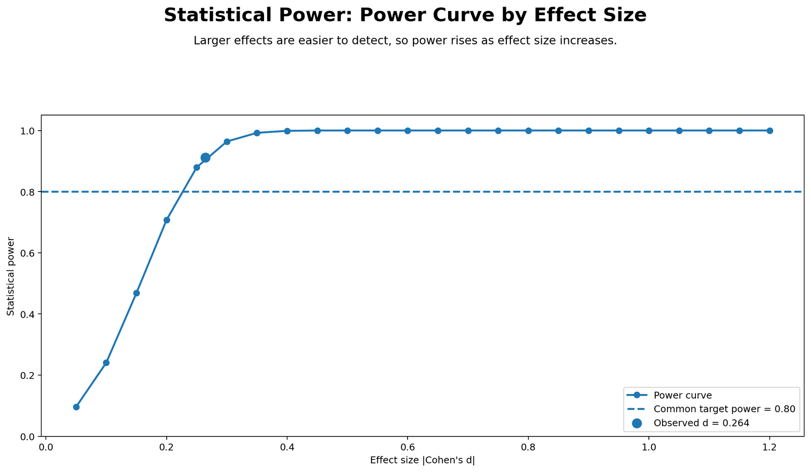
This chart shows the most important idea in Statistical Power: larger effects are easier to detect. When the effect size is small, the power curve stays low unless the sample size is large. As the effect size grows, the test gains sensitivity and power rises toward the common .80 target and then toward 1.00.
The practical interpretation is that a weak or subtle difference requires more participants. A large, clear difference can be detected with fewer observations. Researchers should avoid choosing an unrealistic effect size simply to make the sample size look smaller.
Python Chart 2: Power by Sample Size
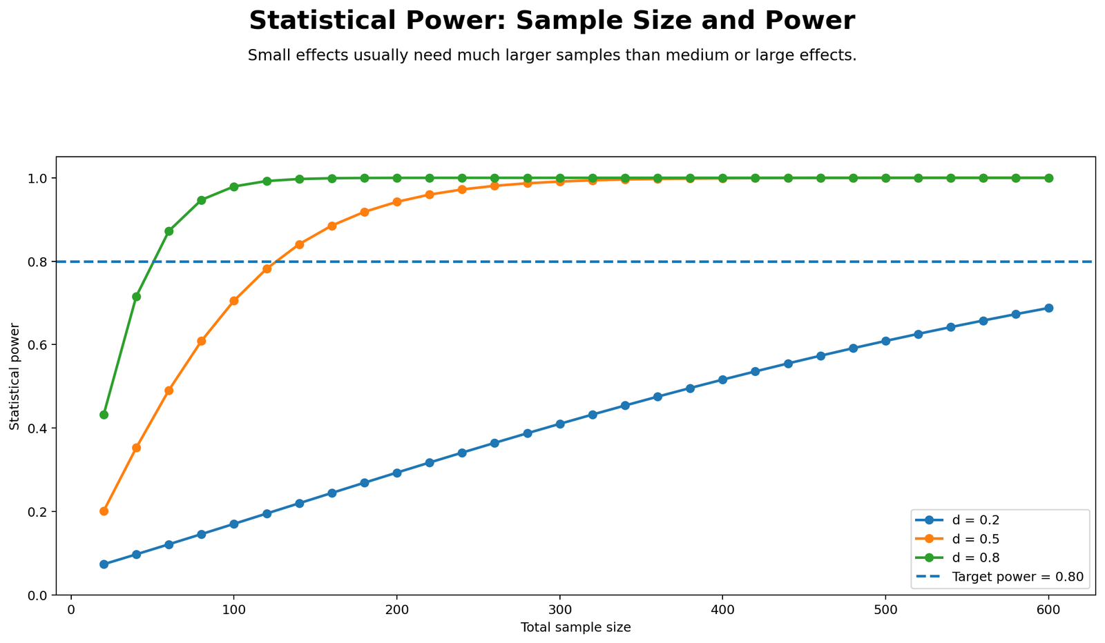
This chart shows how sample size affects Statistical Power. When sample size is small, the study has less information and the test has a lower chance of detecting the effect. As sample size increases, estimates become more stable, standard errors become smaller, and power improves.
The curve usually rises quickly at first and then levels off. This means that adding participants can greatly improve power when the sample is small, but the benefit becomes smaller once the sample is already large. A good design balances statistical sensitivity, cost, time, and ethical constraints.
Python Chart 3: Group Means with Effect Size
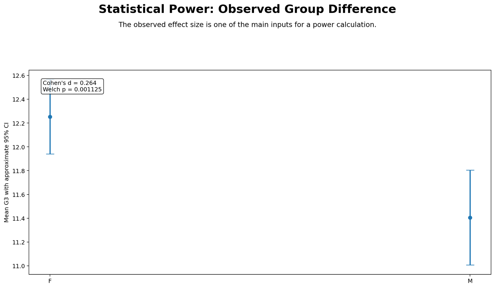
This chart connects Statistical Power with effect size. If the difference between group means is large relative to the spread of scores, the effect size is larger and power improves. If the group means are close together and the distributions overlap heavily, the effect size is smaller and power declines.
This figure is important because power analysis should not be treated as a separate mathematical step. Power depends on the real scientific question: how large is the effect that the researcher wants to detect?
Python Chart 4: Alpha and Power Tradeoff
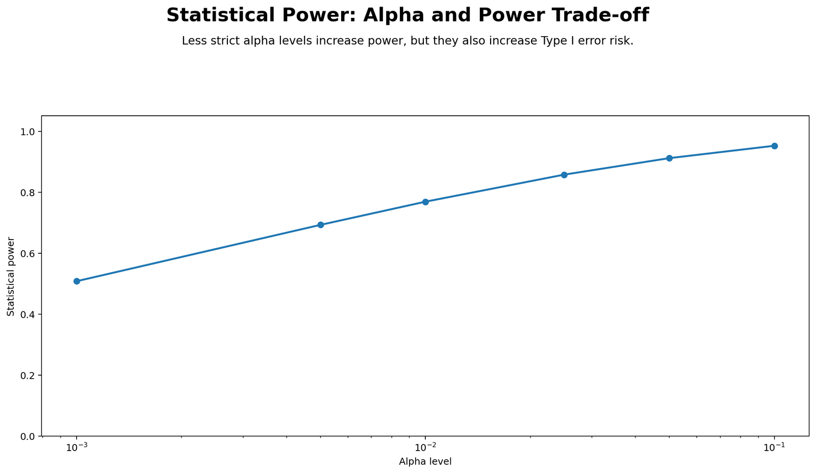
This chart explains the relationship between alpha and Statistical Power. A larger alpha level makes it easier to reject the null hypothesis, so power can increase. However, this also increases the risk of Type I error. A smaller alpha level is more conservative, but it can reduce power unless the sample size is increased.
The correct interpretation is not “raise alpha to get more power.” The correct interpretation is that alpha, power, and sample size must be planned together. If the study needs a strict alpha level, it usually needs a larger sample size to maintain adequate Statistical Power.
Python Chart 5: Power Planning Grid
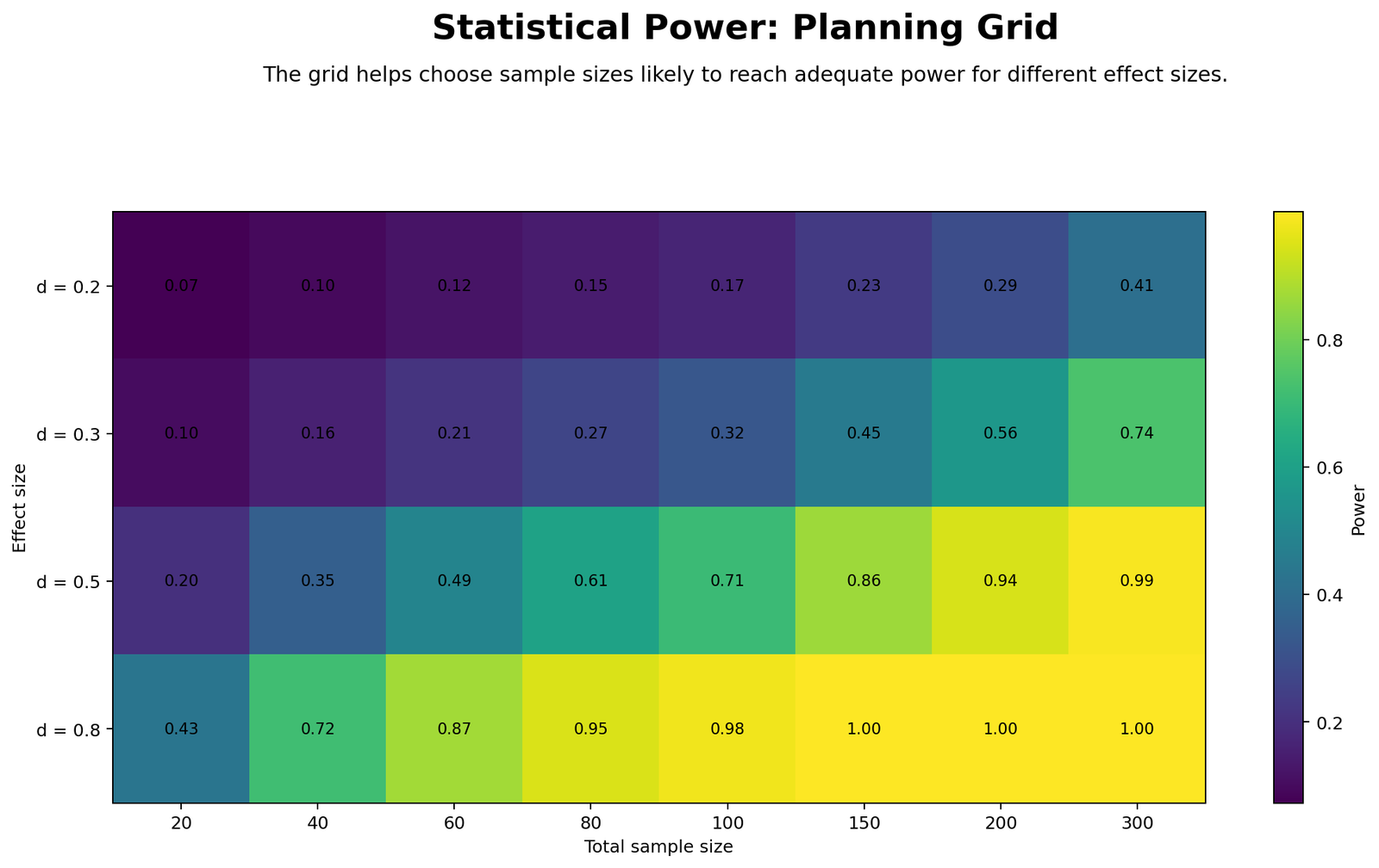
The planning grid shows how Statistical Power changes across combinations of sample size and effect size. It is useful for deciding what sample size is needed for a small, medium, or large effect. A grid format is often clearer than a single power result because it shows what happens if the expected effect is smaller or larger than planned.
For practical research planning, this chart encourages sensitivity analysis. A researcher can ask: “If the true effect is smaller than expected, will the study still have enough power?” This prevents overconfident planning and supports transparent research design.
R Chart-by-Chart Validation
The R charts validate the Python Statistical Power interpretation using a separate workflow. The purpose of R validation is to show that the same power logic appears across software: effect size increases power, sample size increases power, alpha affects power, and planning grids help choose a realistic sample size.
R Chart 1: Power Curve by Effect Size
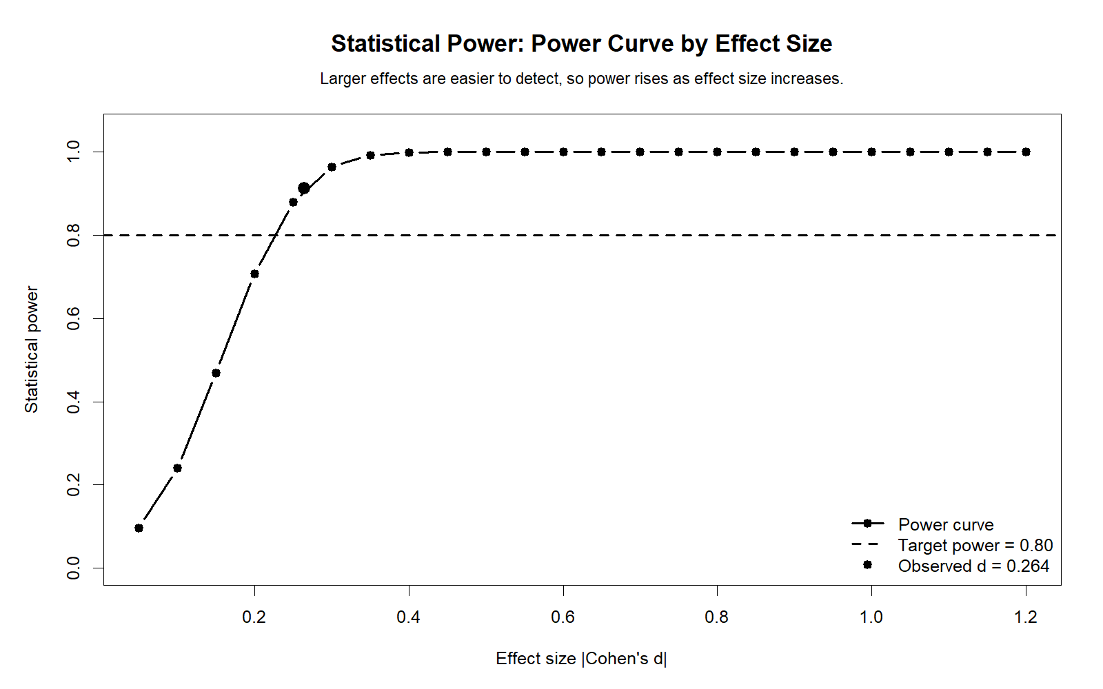
The R power curve confirms the Python result. Small effects produce lower power, while larger effects produce higher power. This validates the core principle that Statistical Power is strongly controlled by the signal strength of the study.
R Chart 2: Power by Sample Size
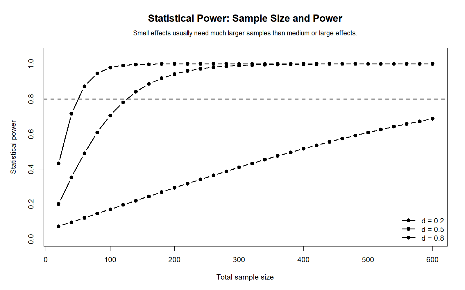
This R chart confirms that larger samples improve Statistical Power. The practical message is the same as the Python chart: when sample size is too small, even a real effect may not be detected.
R Chart 3: Group Means with Effect Size
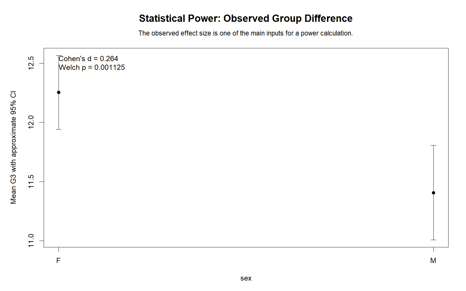
The R group-means chart confirms that power is easier to understand when the actual difference between groups is visible. A larger distance between group means, relative to variability, creates a larger effect size and stronger Statistical Power.
R Chart 4: Alpha and Power Tradeoff
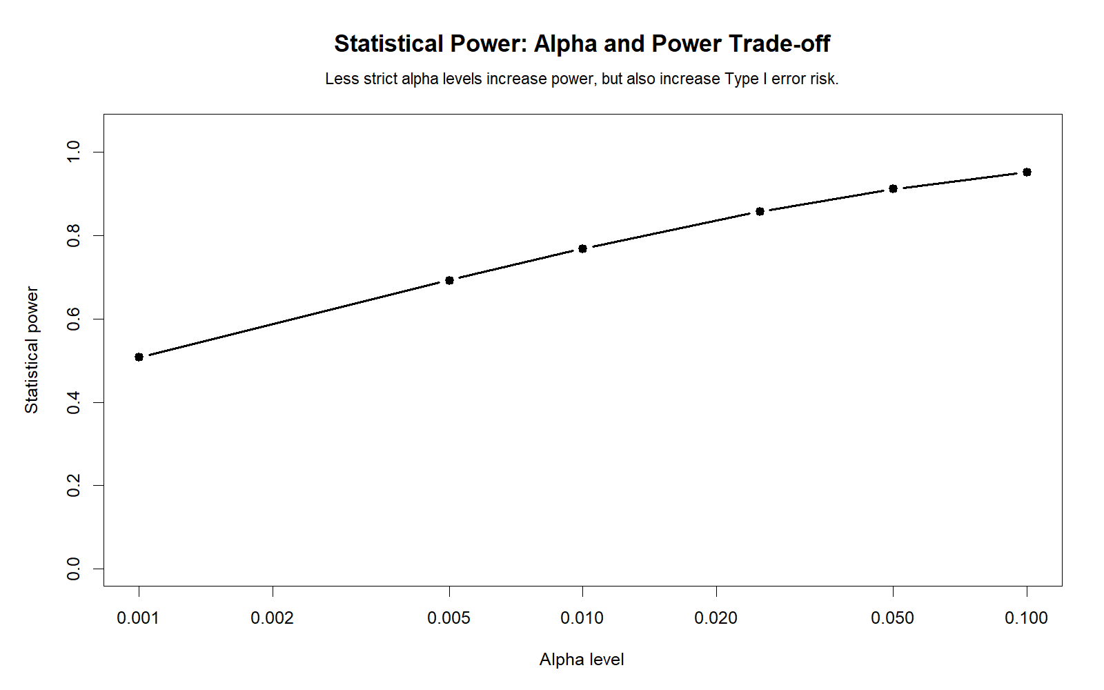
The R alpha tradeoff chart confirms that a less strict alpha can increase power, but the decision must be justified. If alpha is reduced for stronger evidence control, sample size may need to rise to maintain the same power target.
R Chart 5: Power Planning Grid
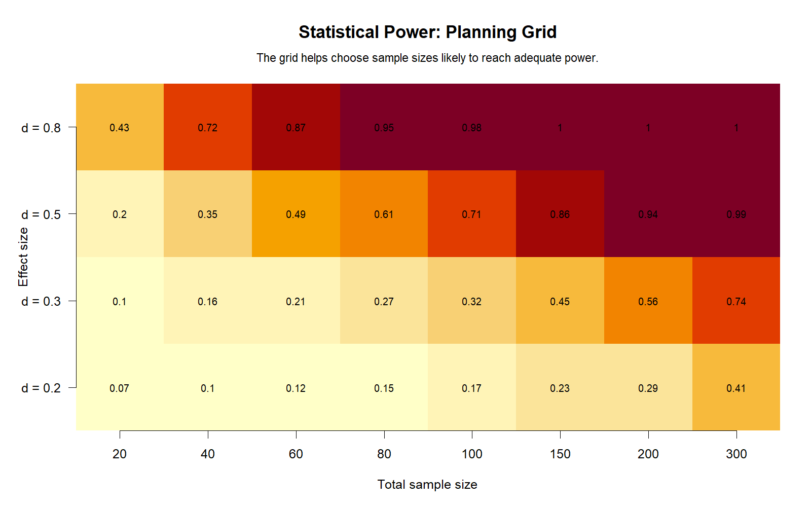
The R planning grid validates the Python planning grid. It shows that sample size recommendations depend on the effect size the researcher wants to detect. This is why Statistical Power should be reported with effect size and not as a standalone number.
SPSS, R, Python and Excel Workflows for Statistical Power
The same Statistical Power analysis can be completed in SPSS, R, Python and Excel. The workflow is always built around the same planning inputs: the test type, effect size, alpha level, power target, and sample size.
SPSS Workflow
| Step | SPSS Action | Purpose |
|---|---|---|
| Choose test | Select the appropriate power analysis procedure | Power must match the actual test, such as t test, correlation, regression or ANOVA. |
| Set alpha | Enter α = .05 or another planned alpha | Controls Type I error and affects Statistical Power. |
| Enter effect size | Use expected Cohen’s d, r, f, odds ratio or regression effect | Defines the effect that the study should detect. |
| Enter sample size or target power | Solve for power or solve for sample size | Determines achieved power or required sample size. |
| Interpret output | Review power, beta and sample size | Decide whether the design is adequately powered. |
| Export PDF | Export the Viewer output | Save the Statistical Power output for reporting. |
R Workflow
| Step | R Action | Purpose |
|---|---|---|
| Install package | install.packages("pwr") | Add power analysis functions. |
| Load package | library(pwr) | Access power functions. |
| Run t-test power | pwr.t.test() | Calculate power or sample size for t tests. |
| Run correlation power | pwr.r.test() | Calculate power for correlation analysis. |
| Create curves | Loop through effect sizes and sample sizes | Visualize Statistical Power across planning choices. |
Python Workflow
| Step | Python Action | Purpose |
|---|---|---|
| Import packages | statsmodels.stats.power | Load power analysis tools. |
| Choose test class | TTestIndPower() or another power class | Match the analysis design. |
| Calculate power | analysis.power() | Compute Statistical Power for given inputs. |
| Solve sample size | analysis.solve_power() | Find required sample size for target power. |
| Create charts | Use matplotlib | Visualize power curves and planning grids. |
Excel Workflow
| Excel Task | Formula or Tool | Purpose |
|---|---|---|
| Enter alpha | Cell value such as 0.05 | Set Type I error level. |
| Enter sample size | Cell value for n per group or total n | Set design size. |
| Enter effect size | Cohen’s d or mean difference divided by pooled SD | Define detectable effect. |
| Calculate critical value | =T.INV.2T(alpha, df) | Find the rejection threshold for a two-tailed t test. |
| Estimate power | Use noncentral t approximation or normal approximation | Approximate Statistical Power for planning. |
| Create grid | Data Table | Compare power across n and effect size. |
Code Blocks for Statistical Power
SPSS Syntax Template for Statistical Power
* Statistical Power workflow template in SPSS.
* Use SPSS power analysis procedures or extension commands where available.
* This template documents planning inputs and exports output.

TITLE "Statistical Power Analysis".

* Example descriptive preparation.
DESCRIPTIVES VARIABLES=G3
  /STATISTICS=MEAN STDDEV MIN MAX.

T-TEST GROUPS=sex('F' 'M')
  /VARIABLES=G3
  /CRITERIA=CI(.95).

* If your SPSS version includes POWER procedures,
* run the relevant POWER command for the selected test.
* Example concept:
* POWER TTEST INDEPENDENT
*   /PARAMETERS TEST=NONDIRECTIONAL SIGNIFICANCE=.05 POWER=.80
*   /ES EFFECT=.30
*   /PLOT TOTAL_N.

OUTPUT EXPORT
  /CONTENTS EXPORT=VISIBLE
  /PDF DOCUMENTFILE="Statistical-Power-SPSS-Output.pdf".
Python Code for Statistical Power
import numpy as np
import pandas as pd
from statsmodels.stats.power import TTestIndPower

analysis = TTestIndPower()

alpha = 0.05
effect_sizes = np.linspace(0.1, 1.0, 10)
sample_sizes = np.arange(20, 301, 20)

# Power by effect size for a fixed sample size per group
n_per_group = 50
power_by_effect = [
    analysis.power(effect_size=d, nobs1=n_per_group, alpha=alpha, ratio=1.0, alternative="two-sided")
    for d in effect_sizes
]

power_effect_table = pd.DataFrame({
    "effect_size_d": effect_sizes,
    "power": power_by_effect
})

print(power_effect_table)

# Required sample size for target power
target_power = 0.80
required_n = analysis.solve_power(
    effect_size=0.5,
    power=target_power,
    alpha=alpha,
    ratio=1.0,
    alternative="two-sided"
)

print("Required n per group:", required_n)

# Power planning grid
rows = []
for d in effect_sizes:
    for n in sample_sizes:
        pwr = analysis.power(effect_size=d, nobs1=n, alpha=alpha, ratio=1.0)
        rows.append({"effect_size_d": d, "n_per_group": n, "power": pwr})

grid = pd.DataFrame(rows)
print(grid.head())
R Code for Statistical Power
# Statistical Power analysis in R

# install.packages("pwr")
library(pwr)

# Power for an independent samples t test
result_power <- pwr.t.test(
  n = 50,
  d = 0.50,
  sig.level = 0.05,
  type = "two.sample",
  alternative = "two.sided"
)

print(result_power)

# Required sample size for 80% power
required_sample <- pwr.t.test(
  d = 0.50,
  power = 0.80,
  sig.level = 0.05,
  type = "two.sample",
  alternative = "two.sided"
)

print(required_sample)

# Power curve across effect sizes
effect_sizes <- seq(0.1, 1.0, by = 0.1)

power_values <- sapply(effect_sizes, function(d) {
  pwr.t.test(
    n = 50,
    d = d,
    sig.level = 0.05,
    type = "two.sample",
    alternative = "two.sided"
  )$power
})

power_table <- data.frame(
  effect_size_d = effect_sizes,
  power = power_values
)

print(power_table)
Excel Formulas for Statistical Power Planning
Step 1:
Enter alpha in a cell:
0.05

Step 2:
Enter expected mean difference:
Mean1 - Mean2

Step 3:
Calculate pooled standard deviation:
=SQRT(((n1-1)*SD1^2 + (n2-1)*SD2^2)/(n1+n2-2))

Step 4:
Calculate Cohen's d:
=(Mean1-Mean2)/Pooled_SD

Step 5:
Calculate standard error:
=Pooled_SD*SQRT(1/n1 + 1/n2)

Step 6:
Calculate test statistic for expected effect:
=(Mean1-Mean2)/Standard_Error

Step 7:
Approximate two-tailed critical z:
=NORM.S.INV(1-alpha/2)

Step 8:
Approximate power:
=1-NORM.S.DIST(Critical_Z - ABS(Expected_Z), TRUE)

Step 9:
Create a planning grid:
Use Data Table with sample size down rows and effect size across columns.
APA Reporting Wording for Statistical Power
APA reporting for Statistical Power should include the test, alpha level, effect size, sample size and power value. If the analysis is an a priori power analysis, say that it was performed before data collection. If the analysis is sensitivity analysis, say what effect size could be detected at the planned power level.
A Priori Power Analysis Wording
An a priori Statistical Power analysis was conducted to estimate the sample size required to detect the expected effect. Using a two-tailed test, α = .05, target power = .80, and the planned effect size, the analysis indicated the minimum sample size required for adequate power. This result was used to guide the study design before final data analysis.
Achieved Power Wording
A Statistical Power analysis was conducted using the observed sample size, alpha level and effect size. The result showed whether the study had adequate sensitivity to detect the observed effect. The power result should be interpreted together with the confidence interval and effect size rather than as a replacement for the main hypothesis test.
Short APA-Style Version
Power analysis indicated that the design approached the common .80 benchmark when the effect size and sample size were sufficiently large. Statistical Power increased as sample size increased and as the expected effect became larger, supporting the need to report both sample size and effect size when interpreting the hypothesis test.
Common Mistakes in Statistical Power Interpretation
| Mistake | Why It Is a Problem | Correct Practice |
|---|---|---|
| Reporting p-value without power | A nonsignificant result may be caused by low power. | Report effect size, confidence interval and Statistical Power context. |
| Choosing an unrealistic effect size | It can make the required sample size look falsely small. | Use prior research, pilot data or a minimum meaningful effect. |
| Confusing alpha with power | Alpha controls Type I error; power controls Type II error risk. | Report alpha and Statistical Power separately. |
| Using observed power as proof of importance | Observed power often repeats information already in the p-value. | Use confidence intervals and effect sizes for practical interpretation. |
| Ignoring one-tailed versus two-tailed tests | Tail direction changes the rejection region and power. | Choose the tail direction before analysis and justify it. |
| Forgetting variability | Noisy data reduce the chance of detecting effects. | Use realistic standard deviations in planning. |
Important warning: High Statistical Power does not prove the effect is meaningful. A very large sample can make a tiny effect statistically significant. Always interpret Statistical Power together with effect size and practical importance.
When to Use Statistical Power
Use Statistical Power whenever you plan a study, justify sample size, interpret a nonsignificant result, compare study designs, or decide whether a statistical test is sensitive enough to detect the effect of interest.
| Use Statistical Power When | Reason | Example |
|---|---|---|
| Planning a study | Determines required sample size. | How many students are needed to detect a grade difference? |
| Interpreting nonsignificant results | Checks whether the test had enough sensitivity. | A p-value above .05 may reflect low power. |
| Choosing between designs | Compares how design choices affect detection ability. | Two-tailed versus one-tailed testing or different group sizes. |
| Writing a thesis or article | Supports sample size justification. | Report alpha, target power and expected effect size. |
| Planning experiments | Reduces wasted resources and Type II error risk. | Estimate required participants before collecting data. |
Statistical Power is especially useful with hypothesis tests such as one-tailed t tests, one sample z tests, one proportion z tests, correlation analysis, ANOVA, regression and clinical research designs. For applied health examples, see clinical trial data analysis using R.
Downloads and Resources for Statistical Power
The SPSS output PDF below verifies the Statistical Power analysis workflow used for this guide. Use it as the supporting output file for SPSS interpretation, power planning, sample size discussion, and reporting.
FAQs About Statistical Power
What is Statistical Power?
Statistical Power is the probability that a test will detect a real effect when that effect truly exists. It is equal to 1 minus beta.
What is a good Statistical Power value?
A common planning benchmark is .80, meaning an 80% chance of detecting the effect if it is real. Some high-stakes studies use .90 or higher.
What does low Statistical Power mean?
Low Statistical Power means the study may fail to detect a real effect. This increases the risk of Type II error.
How is Statistical Power related to Type II error?
Statistical Power equals 1 − β, where β is the probability of Type II error. If beta is .20, power is .80.
Does a larger sample size increase Statistical Power?
Yes. Larger sample size usually increases Statistical Power because it reduces standard error and improves the precision of the estimate.
Does larger effect size increase Statistical Power?
Yes. Larger effects are easier to detect, so Statistical Power increases as effect size increases.
How does alpha affect Statistical Power?
A larger alpha makes rejection easier and can increase power, but it also increases Type I error risk. A smaller alpha is more conservative and may require a larger sample size.
Should Statistical Power be calculated before or after data collection?
The best practice is to calculate Statistical Power before data collection as an a priori sample size plan. Sensitivity analysis can also be useful after sample size is fixed.
Can Statistical Power prove that a result is important?
No. Statistical Power shows detection ability, not practical importance. Practical importance should be judged using effect size, confidence interval and context.
How do I calculate Statistical Power in Python?
Use statsmodels.stats.power, choose the appropriate power analysis class such as TTestIndPower, then enter effect size, sample size, alpha and test direction.
How do I calculate Statistical Power in R?
Use the pwr package. For example, pwr.t.test() calculates power or sample size for t tests.
Can Excel calculate Statistical Power?
Excel can approximate Statistical Power using formulas for effect size, standard error, critical values and normal or t-distribution approximations. For advanced designs, SPSS, R or Python is recommended.

