
Sampling Variability, Mean Precision, Confidence Intervals and Bootstrap Standard Error
Standard Error: Formula, Interpretation, SPSS, Python, R and Excel Guide
Standard Error measures how precisely a sample statistic estimates a population value. The most common version is the Standard Error of the mean, which shows how much the sample mean would vary from sample to sample if the same study were repeated many times. This complete guide explains Standard Error with verified SPSS output, Python charts, R validation charts, Excel workflow, formulas, confidence intervals, bootstrap interpretation, null and alternative hypothesis context, APA reporting wording, common mistakes, downloads, related guides and FAQs.
Quick Answer: Standard Error Result
Standard Error is the estimated sampling variability of a statistic. For a mean, Standard Error is calculated by dividing the sample standard deviation by the square root of the sample size. A smaller Standard Error means the sample mean is more precise. A larger Standard Error means the sample mean has more uncertainty.
In this worked example, the main outcome variable is G3 final grade. The sample contains 649 valid cases. The mean G3 score is approximately 11.91, the standard deviation is approximately 3.23, and the Standard Error of the mean is approximately 0.127. The estimated 95% confidence interval is approximately 11.66 to 12.16. This means the sample mean is estimated with good precision because the sample size is large and the confidence interval is narrow compared with the full spread of G3 scores.
Final interpretation: The Standard Error result shows that the G3 sample mean is estimated with reasonable precision. The raw G3 values vary across students, but the mean itself is stable because the dataset has a large sample size. Therefore, report the mean together with Standard Error and the 95% confidence interval rather than reporting the mean alone.
Important distinction: Standard deviation and Standard Error are not the same. Standard deviation describes the spread of individual G3 scores. Standard Error describes how precisely the sample mean estimates the population mean.
Table of Contents
- What Is Standard Error?
- Standard Error Formula
- Standard Error vs Standard Deviation
- Null and Alternative Hypothesis Context
- Dataset and Variables Used
- Verified SPSS Output Interpretation
- Python Chart-by-Chart Interpretation
- R Chart-by-Chart Validation
- SPSS, R, Python and Excel Workflows
- Code Blocks for Standard Error
- APA Reporting Wording
- Common Mistakes
- When to Use Standard Error
- Downloads and Resources
- Related Guides
- FAQs
What Is Standard Error?
Standard Error is a measure of sampling uncertainty. It tells how much a sample statistic, such as a mean, is expected to vary if repeated samples are taken from the same population. In most beginner and applied data-analysis reports, Standard Error refers to the Standard Error of the mean.
The sample mean is a point estimate. It gives one number, but it does not show uncertainty by itself. Standard Error adds that uncertainty. A small Standard Error means the mean is estimated more precisely. A large Standard Error means the mean is less precise.
Simple definition: Standard Error shows how stable a sample mean is as an estimate of the population mean.
For example, the G3 mean is about 11.91. If we only report the mean, readers know the average final grade, but they do not know how precise that average is. When we report the Standard Error, readers understand that the mean has a measurable amount of sampling uncertainty. When we report the 95% confidence interval, readers get a practical range around that mean.
Standard Error is closely connected with confidence intervals, descriptive statistics, central limit theorem, one sample z test, one-tailed t test, and effect size. When you report a mean, Standard Error helps explain how much uncertainty surrounds that mean.
Standard Error Formula
The most common Standard Error formula is the formula for the Standard Error of the mean:
Here, SD is the sample standard deviation and n is the sample size. The formula shows why Standard Error becomes smaller when the sample size becomes larger. The denominator uses the square root of n, so precision improves as more observations are added.
| Formula Part | Meaning | Effect on Standard Error |
|---|---|---|
| SD | Standard deviation of the sample values | Larger SD increases Standard Error because the raw data are more variable. |
| n | Sample size | Larger n decreases Standard Error because the mean becomes more stable. |
| √n | Square root of sample size | Shows that precision improves gradually, not linearly, as n increases. |
| Mean | Point estimate of the population mean | Standard Error describes uncertainty around this mean. |
Worked Standard Error Example for G3
Using the G3 final grade example, the sample standard deviation is approximately 3.231, and the sample size is 649. The Standard Error is:
Standard Error = SD / sqrt(n)
Standard Error = 3.231 / sqrt(649)
Standard Error ≈ 0.127
This means the sample mean G3 score has an estimated sampling uncertainty of about 0.127 grade points. That value is much smaller than the standard deviation because the standard deviation describes individual variation, while Standard Error describes the uncertainty of the mean.
Standard Error and Confidence Interval Formula
Standard Error is used to build a confidence interval around the mean:
With a large sample, the t multiplier is close to 1.96. Using the G3 values, the approximate 95% confidence interval is:
95% CI ≈ 11.91 ± 1.96 × 0.127
95% CI ≈ 11.91 ± 0.249
95% CI ≈ 11.66 to 12.16
Interpretation: The confidence interval translates Standard Error into a reporting range. Instead of saying only that the mean is 11.91, the report can say that the estimated mean is about 11.91 with a 95% confidence interval from about 11.66 to 12.16.
Standard Error vs Standard Deviation
Standard Error and standard deviation are related, but they answer different questions. Standard deviation describes how spread out individual values are. Standard Error describes how precise the sample mean is as an estimate of the population mean.
| Statistic | Main Question | What It Describes | Common Use |
|---|---|---|---|
| Standard deviation | How spread out are the raw values? | Variation among individual observations | Describing the distribution of scores. |
| Standard Error | How precise is the sample mean? | Sampling uncertainty of the mean | Confidence intervals, error bars, mean precision and hypothesis testing. |
In the G3 example, the standard deviation is about 3.231, while the Standard Error is about 0.127. This large difference is normal because the dataset has many cases. The raw scores vary by several grade points, but the sample mean is estimated much more precisely.
Important: Do not use Standard Error as if it were standard deviation. Standard deviation describes the spread of scores. Standard Error describes the precision of the mean.
Null and Alternative Hypothesis Context
Standard Error itself is not a hypothesis test. However, it is an essential part of many hypothesis tests because it helps calculate the test statistic and confidence interval. When testing a mean against a benchmark, the null and alternative hypotheses are written first, and the Standard Error helps determine whether the observed mean is far enough from the benchmark to reject the null hypothesis.
| Hypothesis Element | Example for Mean G3 | Role of Standard Error |
|---|---|---|
| Null hypothesis | H0: μ = μ0 | Assumes the population mean equals a benchmark or expected value. |
| Alternative hypothesis | H1: μ ≠ μ0 | Assumes the population mean differs from the benchmark. |
| Test statistic | t = (sample mean − benchmark) / Standard Error | Standard Error converts mean difference into a standardized test value. |
| Confidence interval decision | If the benchmark is outside the 95% CI, reject H0 at α = .05 | Standard Error controls the width of the interval. |
SEO and reporting note: In a one sample z test or t test, the Standard Error is not the final decision by itself. It supports the null and alternative hypothesis decision by measuring the uncertainty around the sample mean.
Dataset and Variables Used
The worked Standard Error example uses the student performance dataset. The main variable is G3 final grade. Additional numeric variables such as G1, G2, age and absences are used to compare Standard Error values across variables. Group-level results are used to show how Standard Error changes when means are calculated separately by groups.
| Variable | Role | Why It Matters for Standard Error |
|---|---|---|
| G3 final grade | Main outcome variable | Used to estimate the main mean, Standard Error and 95% confidence interval. |
| G1 and G2 | Additional grade variables | Used to compare Standard Error across related academic variables. |
| age | Numeric background variable | Shows how lower raw spread can produce lower Standard Error. |
| absences | Numeric count variable | Shows how high variability can produce a larger Standard Error. |
| sex or group variable | Comparison category | Used to compare group mean Standard Error and error bars. |
Before interpreting Standard Error, it is useful to review frequency distribution, histogram interpretation, box plot interpretation, five number summary, and coefficient of variation.
Verified SPSS Output Interpretation for Standard Error
The SPSS output PDF verifies the Standard Error workflow. In SPSS, Standard Error usually appears in Explore output, Means output, Descriptives tables, confidence interval tables and group summary tables. The important task is to interpret Standard Error as uncertainty around the sample mean, not as the raw spread of individual scores.
SPSS Descriptive Statistics and Standard Error
| Variable | N | Mean | Standard Deviation | Standard Error | Interpretation |
|---|---|---|---|---|---|
| G1 | 649 | 11.40 | 2.745 | 0.108 | The G1 mean is estimated with good precision because the sample is large. |
| G2 | 649 | 11.57 | 2.914 | 0.114 | The G2 Standard Error is slightly larger than G1 because the SD is larger. |
| G3 | 649 | 11.91 | 3.231 | 0.127 | Main result: the G3 mean is precise relative to the raw spread of scores. |
| age | 649 | 16.74 | 1.218 | 0.048 | Age has a small Standard Error because raw age variation is limited. |
| absences | 649 | 3.66 | 4.641 | 0.182 | Absences has a larger Standard Error because absence counts vary more strongly. |
SPSS Confidence Interval Interpretation
| Statistic | G3 Value | Interpretation |
|---|---|---|
| Mean | 11.91 | The sample estimate of the average final grade. |
| Standard Error | 0.127 | Estimated uncertainty around the G3 mean. |
| 95% Lower Bound | Approximately 11.66 | Lower plausible value for the population mean under 95% confidence. |
| 95% Upper Bound | Approximately 12.16 | Upper plausible value for the population mean under 95% confidence. |
| Practical conclusion | Narrow CI | The mean estimate is reasonably precise for reporting. |
SPSS Group Mean Standard Error Interpretation
SPSS group output should be read by comparing each group’s mean, sample size, standard deviation and Standard Error. A group with fewer cases or greater score variation normally has a wider Standard Error. Therefore, group error bars should be interpreted as mean precision, not as the full range of student scores.
SPSS interpretation summary: The SPSS output supports the interpretation that Standard Error is a precision statistic. The G3 Standard Error is small because the dataset contains 649 cases. The confidence interval around the G3 mean is narrow, which means the mean is stable enough for descriptive reporting.
How SPSS Output Connects with the Charts
The Python and R charts below are visual explanations of the same SPSS logic. The distribution chart shows the mean and confidence interval, the comparison chart shows how Standard Error differs across variables, the confidence interval chart translates Standard Error into interval estimates, the bootstrap chart validates sampling variability, and the group chart shows how Standard Error changes across group means.
Python Chart-by-Chart Interpretation
The Python charts explain Standard Error visually. These figures are not optional decoration; they are the main visual interpretation of the SPSS result. Each figure below uses a real WordPress media URL and is placed inside a proper <figure class="oic-se-figure"> block.
Python Chart 1: Distribution with Mean and Confidence Interval
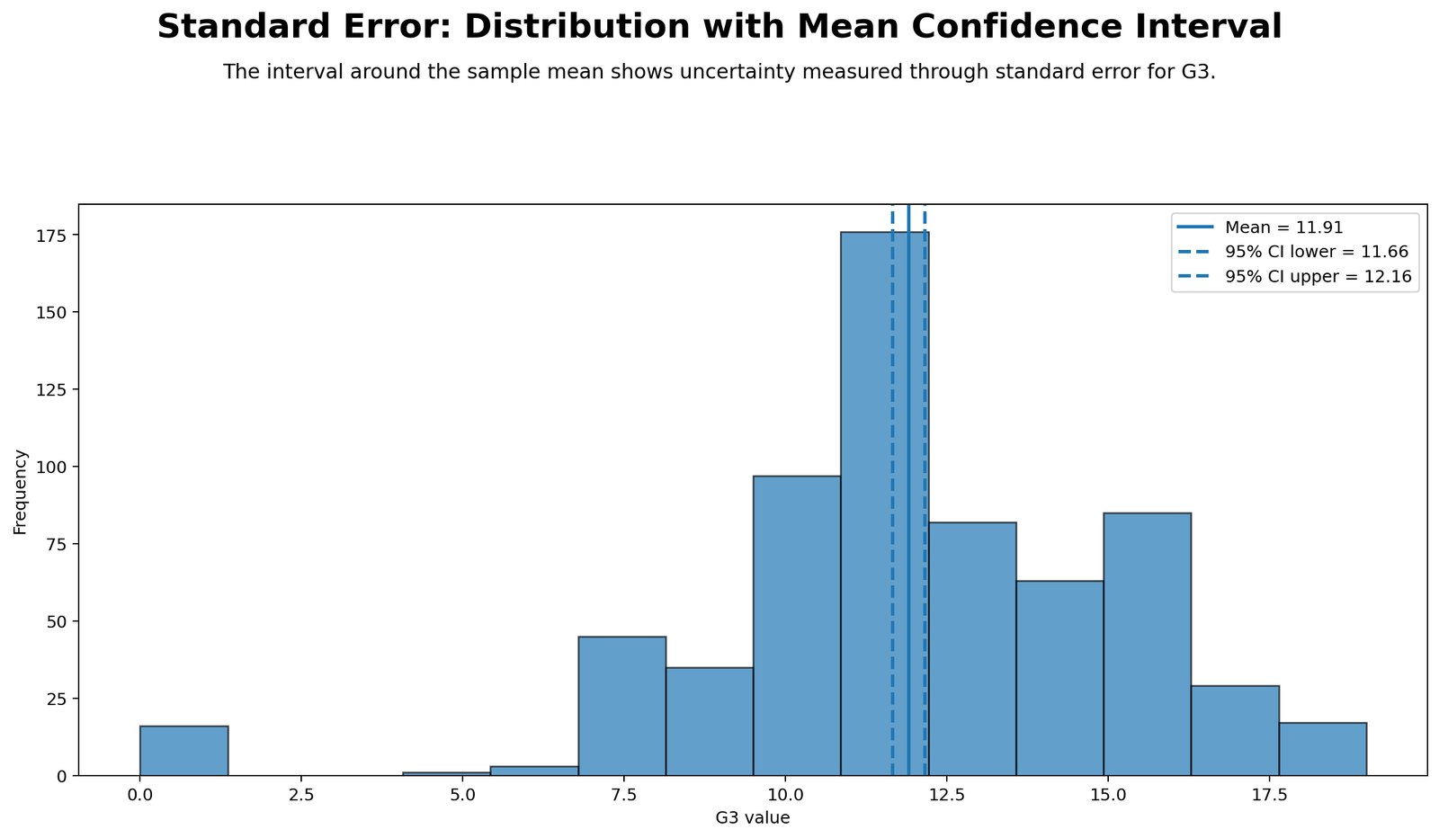
This chart shows how Standard Error connects the sample mean with a confidence interval. The histogram displays the raw distribution of G3 scores, while the mean line marks the point estimate. The confidence interval around the mean is much narrower than the full score distribution because Standard Error measures uncertainty in the mean, not the spread of individual observations.
The correct interpretation is that G3 scores vary across students, but the average G3 score is estimated fairly precisely. The mean line tells where the sample average is located. The confidence interval tells how much uncertainty surrounds that average. The raw histogram tells how much individual students differ from each other. These are three different ideas, and the chart correctly separates them.
This figure also helps explain why a small Standard Error does not mean the raw scores are tightly packed. The G3 distribution still has visible spread, but because there are many cases, the estimated mean has a narrow uncertainty band. That is the key lesson of Standard Error.
Python Chart 2: Standard Error Comparison Across Variables
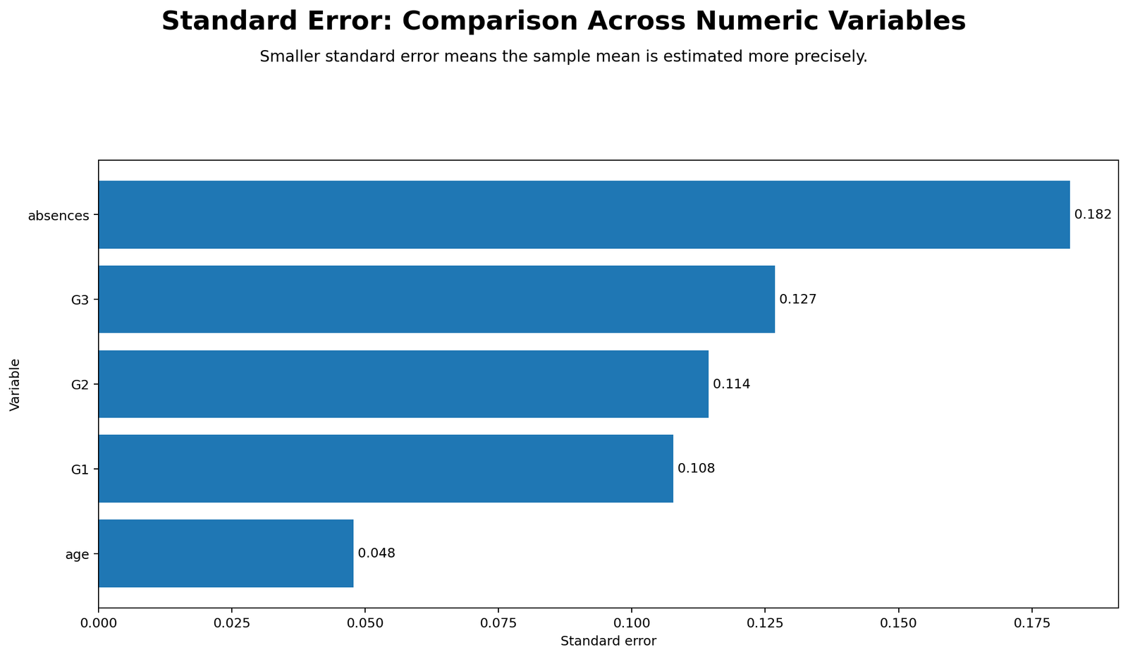
This chart compares Standard Error across several numeric variables. Variables with larger raw spread usually have larger Standard Error, assuming sample size is similar. Since the same dataset has 649 valid cases for the main variables, the differences in Standard Error are mainly driven by differences in standard deviation.
Age has a smaller Standard Error because age has a narrower range and smaller standard deviation. Absences has a larger Standard Error because absence counts are more variable and contain a wider spread. G3 has a moderate Standard Error because final grades vary more than age but less dramatically than highly skewed count variables.
The chart prevents a common reporting mistake: assuming all means are equally precise. They are not. A mean based on a variable with high variability has more uncertainty than a mean based on a variable with low variability, even when sample size is the same.
Python Chart 3: Mean Confidence Intervals
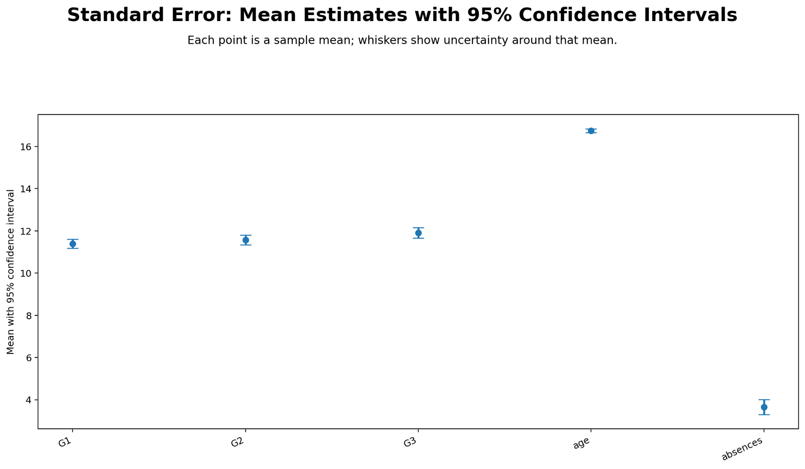
This chart translates Standard Error into confidence intervals. Each point represents a sample mean, and each line around the point represents the uncertainty interval. Narrower intervals show more precise mean estimates. Wider intervals show less precise mean estimates.
For reporting, this chart is often more meaningful than a table of Standard Error values alone. Readers can immediately see which variables have precise means and which variables have wider uncertainty. If a mean has a narrow interval, the estimate is stable. If a mean has a wide interval, the estimate should be interpreted with more caution.
The confidence interval chart also connects Standard Error with hypothesis testing. If a benchmark value falls outside a confidence interval, that can support rejection of the null hypothesis at the corresponding alpha level. If the benchmark falls inside the interval, the evidence against the null benchmark is weaker.
Python Chart 4: Bootstrap Mean Distribution
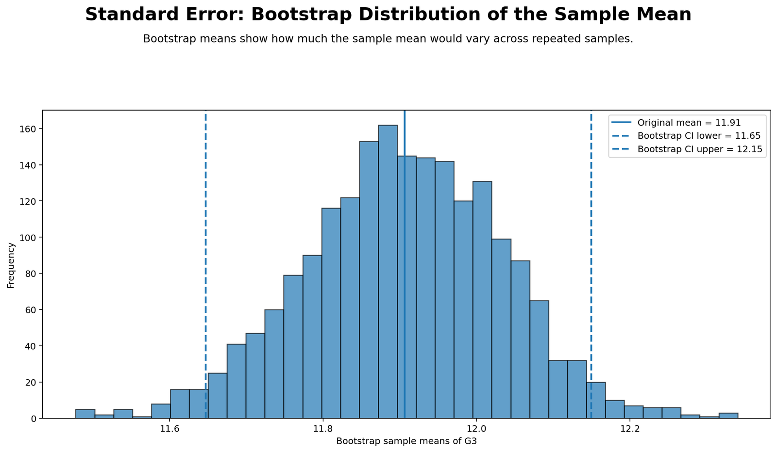
This bootstrap chart explains Standard Error in a very practical way. Instead of relying only on the formula SD / sqrt(n), the bootstrap repeatedly resamples the data and recalculates the mean. The resulting distribution of bootstrap means shows how the sample mean would vary across repeated samples.
If the bootstrap mean distribution is narrow, the mean is stable. If it is wide, the mean has more uncertainty. In this example, the bootstrap distribution is centered near the observed G3 mean and shows a compact spread, supporting the SPSS and formula-based Standard Error result.
This chart is especially helpful for readers who struggle with the abstract idea of sampling variability. It shows that Standard Error is not the spread of raw student scores. It is the spread of possible sample means.
Python Chart 5: Group Mean Standard Error
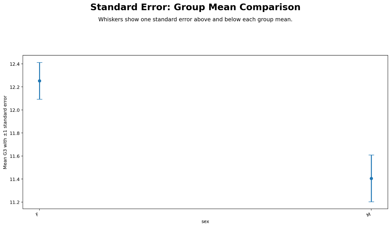
This chart shows group mean Standard Error. Each group mean is displayed with an error bar that represents uncertainty around that group’s mean. Groups with smaller sample size, larger standard deviation or both usually have wider Standard Error bars.
The chart is useful for comparing group precision before moving to formal hypothesis tests. If one group has a visibly wider error bar, its mean is less precise. However, Standard Error bars should not be treated as a complete significance test. They should be interpreted with confidence intervals, effect size and the correct statistical test.
For group comparisons, combine this chart with formal methods such as t tests, confidence intervals, effect size reporting and assumption checks. For example, before comparing group means, it may be useful to review Levene’s test, Brown-Forsythe test, and one-tailed t test guidance.
R Chart-by-Chart Validation
The R charts validate the Python Standard Error interpretation using a separate workflow. The purpose of including R validation is to show that the same result is not dependent on one software package. SPSS, Python and R all support the same conclusion: Standard Error measures mean precision, confidence interval width and sampling variability.
R Chart 1: Distribution with Mean and Confidence Interval
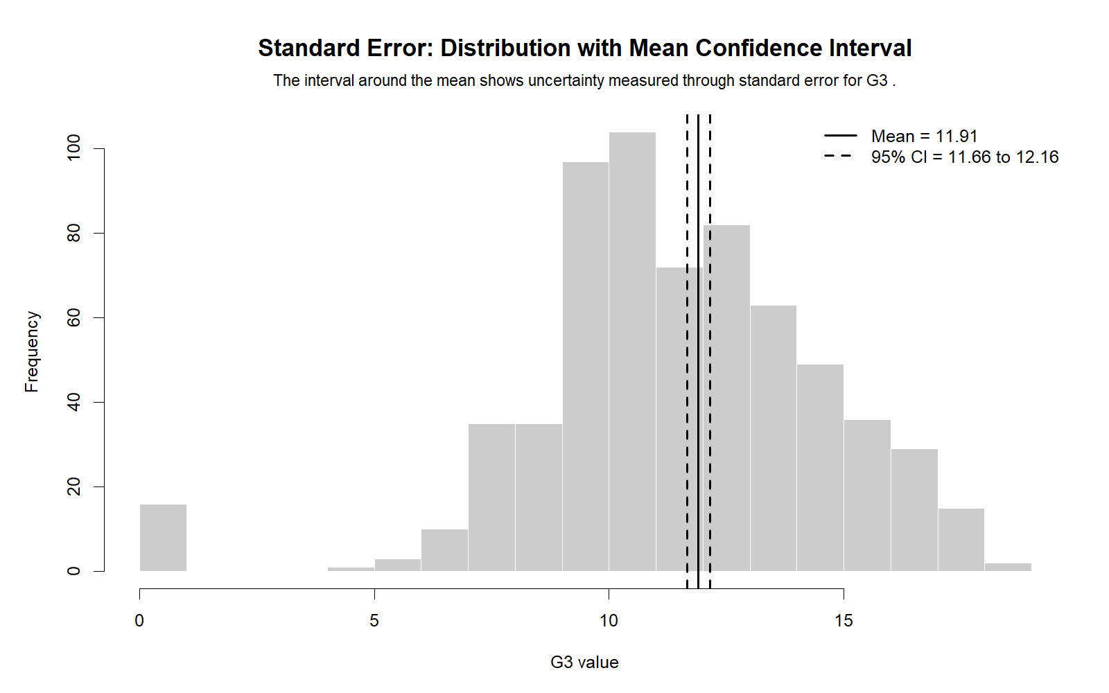
The R distribution chart confirms the same visual message as the Python chart. The raw G3 scores have a visible spread, but the confidence interval around the mean is narrow. This confirms that Standard Error describes the uncertainty around the mean, not the raw spread of students’ grades.
Because the sample size is large, the mean is stable. The R chart validates the formula result and supports reporting the G3 mean with a 95% confidence interval.
R Chart 2: Standard Error Comparison Across Variables
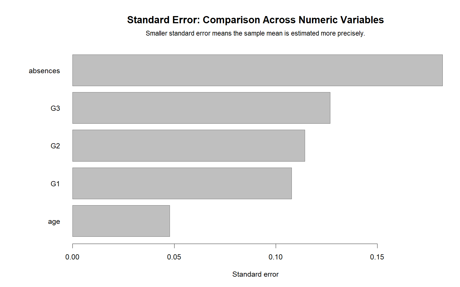
The R comparison chart confirms that Standard Error differs across variables. This happens because the variables have different raw standard deviations. Age has a lower raw spread and therefore a smaller Standard Error. Absences has a wider raw spread and therefore a larger Standard Error.
This validation is useful because it confirms that the comparison is not a Python-only result. The same statistical logic appears when the calculation is performed in R.
R Chart 3: Mean Confidence Intervals
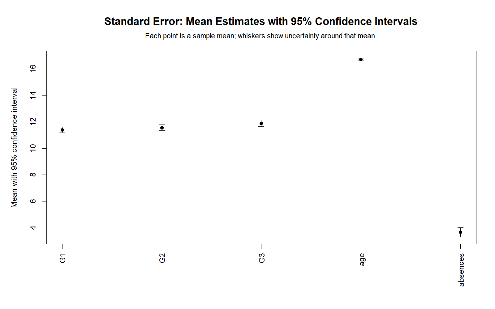
The R confidence interval chart validates the interval-based interpretation. Each interval is created from the mean, t multiplier and Standard Error. When the interval is narrow, the mean estimate is precise. When the interval is wide, the mean estimate has greater uncertainty.
This chart should be used in reporting because readers understand intervals more easily than isolated Standard Error numbers. It also supports better scientific writing because it avoids overconfidence in a single point estimate.
R Chart 4: Bootstrap Mean Distribution
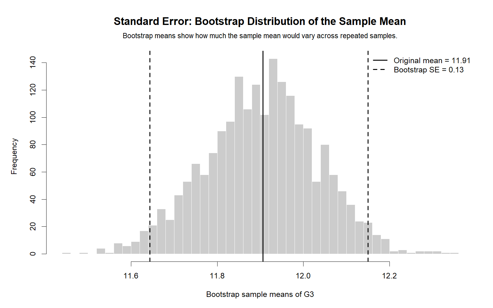
The R bootstrap distribution validates the Python bootstrap result. The spread of resampled means represents sampling variability. This is the practical idea behind Standard Error. If repeated samples produce similar means, the Standard Error is small. If repeated samples produce widely different means, the Standard Error is larger.
The R bootstrap chart strengthens the post because it confirms the formula-based result with a simulation-style approach. This is useful for students, researchers and readers who want a visual explanation rather than only a mathematical formula.
R Chart 5: Group Mean Standard Error
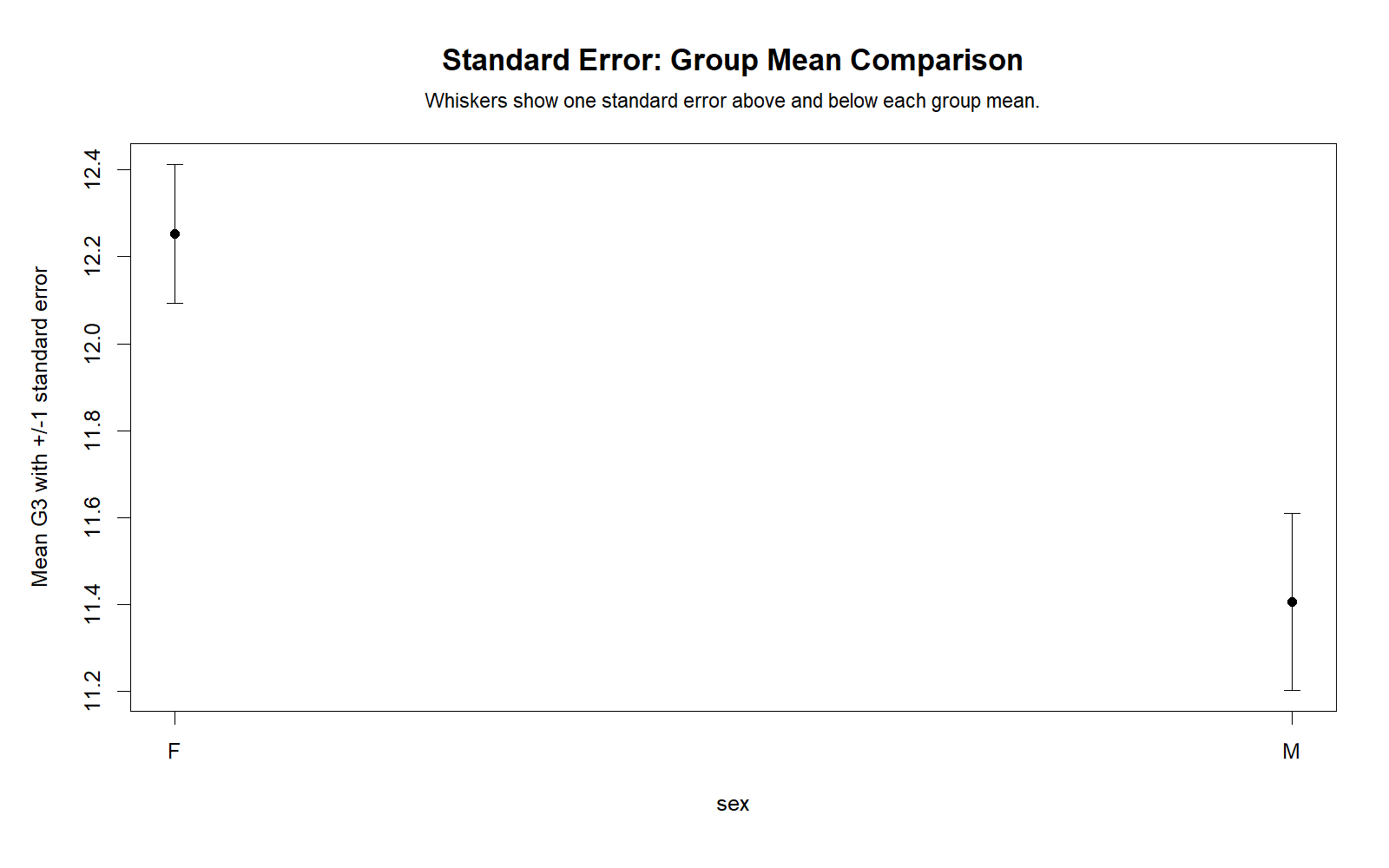
The R group chart confirms that group means can have different levels of precision. The Standard Error bars help readers see which group mean is estimated more or less precisely. A wider error bar means greater uncertainty around that group’s mean.
The R validation chart also helps avoid overinterpreting small group differences. A difference between group means should not be judged only by the height of bars. It should be interpreted with Standard Error, confidence intervals, effect size and the appropriate hypothesis test.
SPSS, R, Python and Excel Workflows for Standard Error
Standard Error can be calculated in SPSS, R, Python and Excel. The workflow is consistent across all tools: calculate the mean, calculate the standard deviation, identify the sample size, compute Standard Error, and then use it to create confidence intervals, error bars or hypothesis-test statistics.
SPSS Workflow
| Step | SPSS Action | Purpose |
|---|---|---|
| Open data | File > Open > Data | Load the clean SPSS-ready dataset. |
| Run Explore | Analyze > Descriptive Statistics > Explore | Generate mean, standard deviation, Standard Error and confidence interval output. |
| Select statistics | Statistics > Descriptives and confidence interval | Obtain the values needed for interpretation. |
| Check groups | Use Factor List or Split File if comparing groups | Calculate group mean Standard Error. |
| Interpret output | Compare mean, SD, SE and confidence interval width | Decide how precise each mean estimate is. |
| Export PDF | File > Export or OUTPUT EXPORT syntax | Save the Standard Error output for reporting. |
R Workflow
| Step | R Action | Purpose |
|---|---|---|
| Read data | read.csv() | Load the dataset into R. |
| Remove missing values | na.omit() | Ensure sample size matches the usable data. |
| Calculate mean | mean(x, na.rm = TRUE) | Find the point estimate. |
| Calculate SD | sd(x, na.rm = TRUE) | Measure raw-score spread. |
| Calculate SE | sd(x) / sqrt(length(x)) | Estimate Standard Error. |
| Create CI | mean ± t * SE | Build confidence interval for the mean. |
Python Workflow
| Step | Python Action | Purpose |
|---|---|---|
| Read data | pandas.read_csv() | Load the dataset into a DataFrame. |
| Select variable | df["G3"].dropna() | Keep valid values only. |
| Calculate mean | series.mean() | Find the sample mean. |
| Calculate SD | series.std(ddof=1) | Find sample standard deviation. |
| Calculate SE | scipy.stats.sem() | Compute Standard Error directly. |
| Create charts | Use matplotlib | Visualize Standard Error, confidence intervals and bootstrap means. |
Excel Workflow
| Excel Task | Formula | Purpose |
|---|---|---|
| Calculate mean | =AVERAGE(range) | Find the sample mean. |
| Calculate sample SD | =STDEV.S(range) | Find spread of the sample values. |
| Calculate sample size | =COUNT(range) | Find n. |
| Calculate Standard Error | =STDEV.S(range)/SQRT(COUNT(range)) | Calculate Standard Error of the mean. |
| Calculate 95% margin of error | =T.INV.2T(0.05,n-1)*SE | Build a confidence interval. |
| Create error bars | Insert chart > Add Chart Element > Error Bars | Show Standard Error bars visually. |
Code Blocks for Standard Error
SPSS Syntax Template for Standard Error
* Standard Error analysis in SPSS.
* Main variable: G3 final grade.

TITLE "Standard Error Analysis".

EXAMINE VARIABLES=G1 G2 G3 age absences
  /STATISTICS=DESCRIPTIVES
  /CINTERVAL=95
  /MISSING=LISTWISE
  /NOTOTAL.

MEANS TABLES=G3 BY sex
  /CELLS=COUNT MEAN STDDEV SEMEAN.

* Optional: one-sample test using Standard Error in the t statistic.
T-TEST
  /TESTVAL=12
  /MISSING=ANALYSIS
  /VARIABLES=G3
  /CRITERIA=CI(.95).

OUTPUT EXPORT
  /CONTENTS EXPORT=VISIBLE
  /PDF DOCUMENTFILE="Standard-Error-SPSS-Output.pdf".
Python Code for Standard Error
import pandas as pd
import numpy as np
from scipy import stats

df = pd.read_csv("dataset.csv")

x = pd.to_numeric(df["G3"], errors="coerce").dropna()

mean_g3 = x.mean()
sd_g3 = x.std(ddof=1)
n_g3 = x.count()
se_g3 = stats.sem(x, nan_policy="omit")

t_crit = stats.t.ppf(0.975, df=n_g3 - 1)
ci_low = mean_g3 - t_crit * se_g3
ci_high = mean_g3 + t_crit * se_g3

print("Mean:", mean_g3)
print("Standard deviation:", sd_g3)
print("Sample size:", n_g3)
print("Standard Error:", se_g3)
print("95% CI:", ci_low, ci_high)

# Standard Error comparison across numeric variables
numeric_vars = ["G1", "G2", "G3", "age", "absences"]

rows = []
for col in numeric_vars:
    s = pd.to_numeric(df[col], errors="coerce").dropna()
    rows.append({
        "variable": col,
        "n": s.count(),
        "mean": s.mean(),
        "sd": s.std(ddof=1),
        "standard_error": s.std(ddof=1) / np.sqrt(s.count())
    })

se_table = pd.DataFrame(rows)
print(se_table)

# Group mean Standard Error
group_summary = df.groupby("sex")["G3"].agg(
    mean="mean",
    sd=lambda s: s.std(ddof=1),
    n="count"
)

group_summary["standard_error"] = group_summary["sd"] / np.sqrt(group_summary["n"])
print(group_summary)

# Bootstrap standard error for the mean
rng = np.random.default_rng(123)
bootstrap_means = []

for i in range(5000):
    sample = rng.choice(x, size=len(x), replace=True)
    bootstrap_means.append(sample.mean())

bootstrap_means = np.array(bootstrap_means)
bootstrap_se = bootstrap_means.std(ddof=1)
bootstrap_ci = np.percentile(bootstrap_means, [2.5, 97.5])

print("Bootstrap SE:", bootstrap_se)
print("Bootstrap 95% CI:", bootstrap_ci)
R Code for Standard Error
# Standard Error analysis in R

df <- read.csv("dataset.csv")

x <- na.omit(as.numeric(df$G3))

mean_g3 <- mean(x)
sd_g3 <- sd(x)
n_g3 <- length(x)
se_g3 <- sd_g3 / sqrt(n_g3)

t_crit <- qt(0.975, df = n_g3 - 1)
ci_low <- mean_g3 - t_crit * se_g3
ci_high <- mean_g3 + t_crit * se_g3

print(mean_g3)
print(sd_g3)
print(n_g3)
print(se_g3)
print(c(ci_low, ci_high))

# Standard Error comparison across variables
numeric_vars <- c("G1", "G2", "G3", "age", "absences")

rows <- lapply(numeric_vars, function(v) {
  z <- na.omit(as.numeric(df[[v]]))
  data.frame(
    variable = v,
    n = length(z),
    mean = mean(z),
    sd = sd(z),
    standard_error = sd(z) / sqrt(length(z))
  )
})

se_table <- do.call(rbind, rows)
print(se_table)

# Group mean Standard Error
group_rows <- aggregate(G3 ~ sex, data = df, function(z) {
  z <- na.omit(as.numeric(z))
  c(mean = mean(z), sd = sd(z), n = length(z), se = sd(z) / sqrt(length(z)))
})

print(group_rows)

# Bootstrap standard error
set.seed(123)
bootstrap_means <- replicate(5000, mean(sample(x, size = length(x), replace = TRUE)))
bootstrap_se <- sd(bootstrap_means)
bootstrap_ci <- quantile(bootstrap_means, probs = c(.025, .975))

print(bootstrap_se)
print(bootstrap_ci)
Excel Formula Block for Standard Error
Assume G3 values are in cells A2:A650.

Mean:
=AVERAGE(A2:A650)

Sample standard deviation:
=STDEV.S(A2:A650)

Sample size:
=COUNT(A2:A650)

Standard Error:
=STDEV.S(A2:A650)/SQRT(COUNT(A2:A650))

95% t critical value:
=T.INV.2T(0.05,COUNT(A2:A650)-1)

Margin of error:
=T.INV.2T(0.05,COUNT(A2:A650)-1)*(STDEV.S(A2:A650)/SQRT(COUNT(A2:A650)))

Lower 95% CI:
=AVERAGE(A2:A650)-Margin_of_Error

Upper 95% CI:
=AVERAGE(A2:A650)+Margin_of_Error

Standard Error bar value:
Use the Standard Error cell as a custom error bar value in Excel charts.
APA Reporting Wording for Standard Error
APA reporting for Standard Error should be clear about whether the value is standard deviation, Standard Error, or confidence interval. Do not write “variation was small” when the number is actually Standard Error. Instead, say that the mean was estimated with a certain level of precision.
APA-Style Descriptive Wording
The mean G3 score was approximately 11.91, with a Standard Error of approximately 0.127. The 95% confidence interval for the mean was approximately [11.66, 12.16], indicating that the sample mean was estimated with reasonable precision.
APA-Style Mean with Standard Error Template
The mean score was M = 11.91, SE = 0.127, 95% CI [11.66, 12.16].APA-Style Group Wording
Group means were reported with Standard Error bars to show uncertainty around each mean. Groups with wider error bars had less precise mean estimates, usually because of smaller sample size, larger variability, or both.
Hypothesis Test Wording Using Standard Error
When the mean was compared with a benchmark value, the Standard Error was used to calculate the test statistic and confidence interval. The null hypothesis stated that the population mean equaled the benchmark, while the alternative hypothesis stated that the population mean differed from the benchmark.
Common Mistakes in Standard Error Interpretation
| Mistake | Why It Is a Problem | Correct Practice |
|---|---|---|
| Confusing Standard Error with standard deviation | They measure different things. | Use SD for raw spread and SE for mean precision. |
| Reporting SE without sample size | SE depends strongly on n. | Report sample size with Standard Error. |
| Using SE bars as a complete significance test | Error bars alone do not replace hypothesis testing. | Use confidence intervals, p-values and effect sizes when needed. |
| Thinking small SE means scores are similar | Small SE can occur because n is large. | Check standard deviation and distribution shape too. |
| Ignoring assumptions | Mean-based inference can be affected by extreme skew or outliers. | Check histograms, boxplots and normality plots. |
| Using SE when CI is clearer | Many readers understand intervals better than isolated SE values. | Report mean, SE and 95% CI together where possible. |
| Comparing SE values across different designs without context | SE depends on design, variance and sample size. | Explain sample size, SD and grouping before comparing SE. |
Important warning: A very small Standard Error does not automatically mean the dataset has low variability. It may only mean the sample size is large. Always compare Standard Error with standard deviation.
When to Use Standard Error
Use Standard Error when you want to explain the precision of a sample statistic. The most common use is reporting the precision of a mean. Standard Error is also used in confidence intervals, hypothesis tests, regression output, bootstrap summaries and group mean charts.
| Use Standard Error When | Reason | Example |
|---|---|---|
| Reporting a mean | Shows uncertainty around the mean. | Mean G3 score with SE and 95% CI. |
| Creating confidence intervals | SE controls interval width. | 95% CI = mean ± t × SE. |
| Comparing group means | Shows which group means are estimated more precisely. | SE bars by sex or study group. |
| Bootstrap analysis | Shows sampling variability from resampled means. | Bootstrap distribution of sample means. |
| Regression and coefficients | SE helps test coefficient uncertainty. | Coefficient divided by SE gives a test statistic. |
| Hypothesis testing | SE helps standardize the difference between the estimate and null value. | One-sample t test or z test. |
Standard Error is also useful after checking assumptions with the Kolmogorov-Smirnov test, Lilliefors test, D’Agostino-Pearson test, Q-Q plot normality check, and P-P plot normality check. For group comparisons, also review the Levene test, Brown-Forsythe test, and Cochran C test.
Downloads and Resources for Standard Error
The SPSS output PDF below verifies the Standard Error workflow used for this guide. Use it as the supporting output file for SPSS interpretation, mean precision, confidence interval discussion, group mean Standard Error and reporting.
Download SPSS Output PDF
Verified SPSS output for Standard Error, descriptive statistics, mean precision and confidence interval interpretation.
Copy Standard Error Code
Use the SPSS, Python, R and Excel code blocks to reproduce the Standard Error analysis.
Download note: Use the SPSS PDF as the official verification file. The Python and R charts provide visual interpretation and software validation for the same Standard Error decision.
FAQs About Standard Error
What is Standard Error?
Standard Error is the estimated sampling variability of a statistic. For a mean, it shows how precisely the sample mean estimates the population mean.
What is the formula for Standard Error?
The most common formula is Standard Error = SD / √n, where SD is the sample standard deviation and n is the sample size.
What does a small Standard Error mean?
A small Standard Error means the sample mean is estimated more precisely. It does not necessarily mean that individual values have low variability.
What does a large Standard Error mean?
A large Standard Error means the sample mean has more uncertainty. This may happen because the sample size is small, the data are highly variable, or both.
Is Standard Error the same as standard deviation?
No. Standard deviation describes the spread of individual values. Standard Error describes the uncertainty of the sample mean.
How is Standard Error used in confidence intervals?
Standard Error is multiplied by a critical value and added to and subtracted from the mean to create a confidence interval.
Does sample size affect Standard Error?
Yes. Larger sample size reduces Standard Error because the denominator of the formula is the square root of n.
What was the Standard Error for G3 in this example?
The G3 Standard Error was approximately 0.127, based on a standard deviation of about 3.231 and a sample size of 649.
What is the 95% confidence interval for the G3 mean?
The approximate 95% confidence interval for the G3 mean was about 11.66 to 12.16.
How do I calculate Standard Error in Excel?
Use =STDEV.S(range)/SQRT(COUNT(range)) to calculate the Standard Error of the mean in Excel.
How do I calculate Standard Error in Python?
Use scipy.stats.sem() or calculate series.std(ddof=1) / sqrt(n).
How do I calculate Standard Error in R?
Use sd(x) / sqrt(length(x)) after removing missing values.
Should I report Standard Error or confidence interval?
For most research reports, confidence intervals are clearer because they show the range of likely values. You can report both mean, Standard Error, and 95% CI when needed.
Can Standard Error be shown with error bars?
Yes. Standard Error bars can show uncertainty around means, but they should not be treated as a complete significance test.
Does Standard Error test the null hypothesis?
No. Standard Error is not a hypothesis test by itself. It helps calculate test statistics and confidence intervals used in null and alternative hypothesis decisions.

