
Reliability Analysis in R: Standardized Alpha, R Code and Interpretation
Reliability analysis in R evaluates whether a set of scored items behaves consistently enough to justify a common scale score. This R-only guide develops a complete worked analysis for six transformed student-life items, shows how the correlation matrix produces standardized Cronbach alpha, explains every supplied R chart, and demonstrates how to diagnose a low coefficient without hiding multidimensional item behavior.
The six items show weak internal consistency after standardization.
The worked reliability analysis in R uses 649 complete records and six scored variables: famrel, freetime, goout, Dalc_R, Walc_R, and health. The mean of the 15 unique inter-item correlations is 0.032763. With six items, the standardized alpha formula returns 0.168910.
This result is not evidence that R failed. It indicates that the selected items do not behave like interchangeable indicators of one narrow latent construct. The matrix contains a strong positive association between reversed workday and weekend alcohol items, a moderate positive association between free time and going out, and several negative cross-domain relationships. Reliability analysis in R therefore reveals a scale-definition problem rather than a software problem.
Verified R metrics
What reliability analysis in R measures
Internal consistency is a property of scores from a defined item set, population, administration and scoring rule.
Reliability analysis in R asks whether several observed items contain enough shared variation to support their interpretation as a composite scale. The analysis is often summarized with Cronbach alpha, standardized alpha, mean inter-item correlation, corrected item-total correlations, and alpha-if-item-deleted values. These statistics do not prove validity, unidimensionality, accuracy or causal meaning. They describe how the item scores co-vary in the analyzed sample.
Consistency is not sameness
Items in a useful scale do not need identical distributions or identical wording. They should, however, move together in a pattern that fits the intended construct. When respondents score relatively high on one favorable item, they should generally score relatively high on other favorable items after negatively phrased items have been reversed. A reliability analysis in R quantifies this shared movement while preserving enough detail to locate contradictory item pairs.
Very high correlations can also be undesirable when they reflect duplicated wording rather than broad construct coverage. Reliability is therefore a balance: enough common variance for a coherent score, but not so much redundancy that several items merely repeat the same question.
What alpha summarizes
Cronbach alpha is a function of the number of items and their average covariance or correlation. Standardized alpha uses the correlation matrix, so every item is placed on a variance-one scale before the coefficient is computed. In reliability analysis in R, standardized alpha is especially useful when items have different units, ranges or variances but are intended to have equal conceptual weight.
Alpha rises when the item count rises, when average inter-item association rises, or both. A large alpha can therefore result from many weakly related items, while a short focused scale can have a moderate alpha despite clear content coherence. Interpretation must always return to the matrix and construct definition.
A reliability coefficient is also not a test of whether every correlation differs significantly from zero. With 649 cases, small correlations can be statistically detectable while remaining too small to support a coherent scale. The present workflow emphasizes magnitude, direction, dimensional pattern and practical interpretation rather than treating a p-value as the main decision rule.
Researchers sometimes say that alpha measures how “accurately” a scale measures a construct. That wording is too broad. Accuracy involves validity, calibration, bias and criterion relationships. Reliability analysis in R focuses more narrowly on consistency of the observed item scores. A scale may be consistent but measure the wrong construct, and it may measure a valuable broad domain while showing low alpha because the domain contains distinct facets.
When to use reliability analysis in R
Use internal-consistency methods only when a defensible common score is being considered.
Reliability analysis in R is appropriate when several items are intended to represent one construct or a clearly defined subscale. Typical applications include questionnaire domains, attitude scales, symptom inventories, knowledge-test sections, classroom rubrics and multi-item behavioral indices. The data should contain one row per respondent or observational unit and one column per scored item.
Good use
Use the analysis when theory predicts that all selected items should respond to the same underlying attribute. Examples include several questions about academic confidence, several ratings of service responsiveness, or several tasks designed to assess one skill. In these settings, reliability analysis in R helps determine whether a total or average score is defensible.
Questionable use
Be cautious when items deliberately cover different dimensions. A broad “student life” index combining family relations, free time, social activity, alcohol behavior and health may be meaningful as a profile, but the components need not correlate strongly. Low alpha can be expected because diversity is built into the content rather than caused by measurement noise.
Wrong use
Do not use alpha as an agreement coefficient for several judges, as a stability coefficient across time, or as a substitute for factor analysis. Inter-rater agreement, test-retest stability and dimensionality answer different questions. The related-guides section links to methods that match those designs.
The first decision in reliability analysis in R is not which function to call. It is whether the items should be combined at all. Review the questionnaire, coding guide and construct map before calculating anything. Identify reverse-keyed items, confirm the intended direction of high scores, separate subscales, and document whether each item is reflective or formative.
Reflective items are viewed as effects of a common underlying construct, so internal correlation is expected. Formative indicators jointly define an index and may not correlate. Household income, education and housing quality, for example, can contribute to a socioeconomic index without behaving as interchangeable reflections. Applying reliability analysis in R to formative indicators can wrongly penalize useful diversity.
| Research design | Primary question | Recommended direction |
|---|---|---|
| Several questionnaire items, one proposed scale | Do items show internal consistency? | Use reliability analysis, item diagnostics and dimensional checks. |
| Same scale administered twice | Are scores stable over time? | Use test-retest correlation or an appropriate agreement coefficient. |
| Several raters score the same cases | Do raters agree? | Use an intraclass correlation or categorical agreement method. |
| Items may represent several factors | How many dimensions are present? | Use factor analysis before or beside alpha. |
| Indicators deliberately define a broad index | Do components jointly cover the domain? | Use content and criterion evidence rather than alpha alone. |
Variables used in the reliability analysis in R example
Six complete ordinal-style variables are analyzed after two alcohol-use items are reversed.
The worked reliability analysis in R uses 649 student records and six variables. The first three describe family and social context, two represent reverse-scored alcohol-use frequencies, and one records perceived health. Each original item uses a five-point scale. Reversing the alcohol variables makes larger values represent lower alcohol consumption, so all items are oriented toward a more favorable or regulated direction before the correlation matrix is calculated.
| R variable | Meaning | Original coding | Analysis coding | High-score interpretation |
|---|---|---|---|---|
| famrel | Quality of family relationships | 1 = very bad to 5 = excellent | Unchanged | Better family relationships |
| freetime | Free time after school | 1 = very low to 5 = very high | Unchanged | More free time |
| goout | Going out with friends | 1 = very low to 5 = very high | Unchanged | More social outings |
| Dalc_R | Reverse-scored workday alcohol consumption | Original Dalc: 1 = very low to 5 = very high | Dalc_R = 6 – Dalc | Lower workday alcohol consumption |
| Walc_R | Reverse-scored weekend alcohol consumption | Original Walc: 1 = very low to 5 = very high | Walc_R = 6 – Walc | Lower weekend alcohol consumption |
| health | Current health status | 1 = very bad to 5 = very good | Unchanged | Better perceived health |
Why Dalc and Walc were reversed
Without reversal, high alcohol-consumption values would point in the opposite substantive direction from favorable family and health values. The transformation 6 – original score preserves the five response categories while switching their order. A response of 1 becomes 5, 2 becomes 4, 3 remains 3, 4 becomes 2 and 5 becomes 1.
Direction should be decided from the scoring theory before reliability analysis in R. Automatic key detection can identify negative correlations, but it cannot decide whether an item belongs in the construct. Reversing a poorly chosen item may change the sign without fixing conceptual mismatch.
Why reversal did not produce high alpha
Reverse coding aligns direction, but it does not manufacture a common factor. In the verified matrix, Dalc_R and Walc_R correlate 0.617 because workday and weekend alcohol behavior are closely related. However, goout correlates -0.245 with Dalc_R and -0.389 with Walc_R after reversal. Students who go out more tend to have lower reverse-coded alcohol scores, which is substantively plausible but inconsistent with treating every item as an interchangeable favorable indicator.
The resulting reliability analysis in R therefore retains several negative cross-domain correlations and yields low standardized alpha.
The exact variable labels belong in reporting because generic labels such as “item 1” and “item 2” conceal the content pattern. The correlation matrix shows two local clusters: freetime with goout, and Dalc_R with Walc_R. Family relations and health have only small positive associations with most other variables. This structure is more informative than the single coefficient.
Prepare data before reliability analysis in R
Reliable output requires correct rows, numeric items, direction, missing-value rules and variation checks.
Data preparation for reliability analysis in R begins with a rectangular item matrix. Each row should represent one independent respondent and each column one item intended for the same scale or subscale. Identification fields, grouping variables, demographic categories and outcomes should not be accidentally included in the reliability function.
Select the scale
Choose items from the scoring key and construct map, not from whichever numeric columns are easiest to access.
Confirm direction
Reverse negatively keyed variables using the documented response range before calculating correlations.
Check numeric types
Convert imported character or factor columns carefully and verify that category labels were not converted to incorrect integers.
Define missingness
Choose listwise or pairwise handling deliberately and report the number of records used by the final matrix.
Inspect distributions
Check ranges, zero-variance items, sparse categories, floor or ceiling effects, and unexpected values.
items <- c("famrel", "freetime", "goout", "Dalc_R", "Walc_R", "health")# Reverse the original 1-to-5 alcohol-use items when needed.
dat$Dalc_R <- 6 - dat$Dalc
dat$Walc_R <- 6 - dat$Walc
# Create the analysis matrix and force numeric storage safely.
x <- dat[items]
x[] <- lapply(x, function(z) as.numeric(as.character(z)))
# Use complete records for one common correlation matrix.
x_complete <- x[complete.cases(x), ]
nrow(x_complete) # 649
ncol(x_complete) # 6
sapply(x_complete, range, na.rm = TRUE)
sapply(x_complete, sd, na.rm = TRUE)
Listwise deletion produces one common set of 649 cases for all 15 item pairs. This makes the standardized-alpha formula internally coherent because every correlation is based on the same records. Pairwise deletion can retain more data, but each correlation may then use a different subset. If missingness is substantial, the resulting matrix may not correspond to any actual common sample and can even become non-positive definite.
For ordinal five-category items, Pearson correlations are frequently used in conventional alpha calculations, especially when distributions are not extremely skewed. However, a reliability analysis in R can also use polychoric correlations when items are treated as manifestations of underlying continuous variables. The choice changes the estimand. It should be justified by measurement theory, category distributions and sample size rather than selected because it produces a preferred coefficient.
Range and coding audit
Every item in this example should remain between 1 and 5 after transformation. Values outside that range suggest data-entry or import errors. The reversed variables should still have five categories and the same missing-value locations as their originals. Frequency tables are useful because a simple mean can hide an impossible value offset by other observations.
Before reliability analysis in R, compare original and reversed variables with a small cross-tabulation. Confirm that 1 maps to 5 and 5 maps to 1. Do not overwrite original fields unless the data-management plan explicitly requires it.
Variance and ceiling effects
An item with nearly no variation cannot correlate strongly with the rest because respondents provide little information for distinguishing scores. Severe ceiling or floor effects compress covariance. In this example, the items have usable variation, but their substantive relationships differ. The low coefficient is therefore mainly explained by mixed correlation signs and weak average association rather than a single constant item.
Use variance, standard deviation and distribution plots beside the matrix.
Standardized alpha formula for reliability analysis in R
The verified coefficient follows directly from six items and their average unique correlation.
Standardized alpha in reliability analysis in R uses the average inter-item correlation rather than the raw covariance matrix. Let k be the number of items and let r̄ be the mean of the correlations above the diagonal. The coefficient is:
The diagonal values of 1 are not averaged because they are each item correlated with itself. With six items, the matrix contains 6 × 5 / 2 = 15 unique off-diagonal pairs.
The substitution reproduces the R report to rounding precision. The low numerator reflects a very small mean inter-item correlation.
Why item count matters
For a fixed positive r̄, alpha increases as items are added because a longer scale averages more item-specific variation. This is the same logic summarized by the Spearman-Brown formula. Lengthening a scale can improve reliability only when added items share the intended construct. Adding unrelated items may lower r̄ enough to offset the benefit of length.
In this reliability analysis in R, six items are not enough to compensate for an average correlation near zero. The remedy is not to add arbitrary columns. It is to define coherent subdomains and develop items that represent each domain consistently.
Why negative pairs matter
The mean correlation is an algebraic average. Positive and negative pairs can cancel. Here, Dalc_R and Walc_R contribute a strong 0.617, while goout with Walc_R contributes -0.389 and goout with Dalc_R contributes -0.245. A coefficient of 0.168910 therefore compresses a matrix containing both meaningful positive clusters and meaningful negative relationships.
That is why reliability analysis in R should never stop at the summary coefficient. The matrix explains which pairs create the result.
Raw alpha versus standardized alpha
Raw Cronbach alpha uses item variances and covariances. Standardized alpha uses correlations and is equivalent to computing raw alpha after every item is standardized to variance one. When all items share the same response scale and have similar variances, the two coefficients are often close. When variances differ substantially, they can diverge.
The present guide centers on standardized alpha because the supplied reliability analysis in R report is explicitly a correlation-matrix workflow. Standardization removes raw variance differences, but it does not remove multidimensionality, reverse-direction errors or weak relationships. A low standardized coefficient therefore cannot be blamed on unequal item variances.
Alpha is bounded above by 1 under conventional positive-semidefinite conditions, but it can be negative when the average covariance is negative. Negative alpha is usually a sign of incorrect direction, severe multidimensionality or an item set that should not be combined. Positive but low alpha, as in this example, points to the same issues in a less extreme form.
How to run reliability analysis in R
Base R reproduces the standardized result transparently; a specialist package adds item diagnostics.
The clearest way to learn how to run reliability analysis in R is to compute the correlation matrix, extract its unique upper-triangle values, calculate their mean and substitute that value into the standardized-alpha equation. This approach exposes every step and avoids treating a package function as a black box.
# Items already oriented so larger values have the intended direction.
items <- c("famrel", "freetime", "goout", "Dalc_R", "Walc_R", "health")
x <- dat[items]
x <- x[complete.cases(x), ]# Standardized correlation matrix.
R <- cor(x, use = "complete.obs", method = "pearson")
# Mean of the 15 unique off-diagonal correlations.
upper_r <- R[upper.tri(R)]
mean_inter_item_r <- mean(upper_r)
# Standardized Cronbach alpha.
k <- ncol(x)
standardized_alpha <- (k * mean_inter_item_r) /
(1 + (k - 1) * mean_inter_item_r)
list(
standardized_alpha = standardized_alpha,
mean_inter_item_r = mean_inter_item_r,
items = k,
n_cases = nrow(x),
correlation_matrix = R
)
The expected values are standardized_alpha = 0.168909570161064, mean_inter_item_r = 0.0327632892853925, items = 6 and n_cases = 649. Printing more digits during verification is useful; reporting three decimals is usually sufficient for an article or research report.
# install.packages("psych") # Run once when the package is not installed.
library(psych)items <- c("famrel", "freetime", "goout", "Dalc_R", "Walc_R", "health")
x <- dat[items]
x <- x[complete.cases(x), ]
fit <- psych::alpha(
x,
check.keys = FALSE,
warnings = TRUE,
n.iter = 1000
)
fit$total[c("raw_alpha", "std.alpha", "average_r", "nvar")]
fit$item.stats
fit$alpha.drop
fit$keys
Set check.keys = FALSE when item direction has already been established and reversed deliberately. Setting it to TRUE lets the function search for negatively keyed items, but automated reversal is exploratory. It can increase alpha by changing signs even when the item is conceptually outside the construct. A defensible reliability analysis in R records the scoring decision before fitting the model.
Read the total output
The total component contains raw alpha, standardized alpha, average correlation, signal-to-noise ratio and scale summaries. Match std.alpha with the base R calculation. If they differ, check missing-data handling, selected columns and whether the package reversed any items.
The average_r value should equal the mean of the upper triangle of the same matrix. In this example it is approximately 0.032763.
Read the item output
The item.stats and alpha.drop components show item means, standard deviations, corrected item-total correlations and coefficients after deleting each item. These diagnostics identify unusual items, but deletion must be driven by content and dimensional evidence. A larger alpha after removal does not automatically justify removal.
Use the separate corrected item-total correlation guide for detailed interpretation.
For scripted projects, save the item list, sample count, matrix, alpha summary and session information. Reproducibility matters because package versions, automatic keying and missing-value options can change output. A reliable script should fail clearly when required columns are missing or when an item has zero variance.
stopifnot(all(items %in% names(dat)))

stopifnot(ncol(x) >= 2)

stopifnot(all(vapply(x, is.numeric, logical(1))))

stopifnot(all(vapply(x, function(z) sd(z) > 0, logical(1))))

stopifnot(nrow(x) == 649)

stopifnot(abs(standardized_alpha - 0.168909570161064) < 1e-12)How to interpret the reliability analysis in R output
Interpret the coefficient, average correlation, pairwise structure, item count and sample together.
The main conclusion from this reliability analysis in R is that the six-item composite has weak standardized internal consistency. The coefficient of 0.168910 lies close to zero and far below values commonly expected when items are intended as interchangeable reflections of one narrow construct. The mean inter-item correlation of 0.032763 shows why: the average pair shares very little linear variation.
Statistical interpretation
The standardized coefficient indicates that the equally weighted, standardized items do not form a strongly homogeneous scale. Because alpha is a descriptive function of the matrix, there is no separate rejection decision required. The practical question is whether the coefficient and item pattern are adequate for the intended use, stakes and construct breadth.
In a high-stakes individual decision, 0.169 would be unacceptable. In an exploratory profile where the six variables are not expected to be interchangeable, alpha may simply be the wrong criterion.
Substantive conclusion
The six items contain distinct social, behavioral and wellbeing components. A single unqualified total would conceal their opposing relationships.
Review construct and subscales
Conventional rules such as 0.70 for “acceptable” reliability are sometimes useful as rough communication devices, but they are not universal laws. A coefficient must be judged against the intended decisions, number of items, construct breadth, score distribution and consequences of error. Reliability analysis in R is strongest when it reports the continuous coefficient and supporting diagnostics rather than converting the result into a simplistic pass-fail label.
The sample size of 649 provides stable estimation of the matrix, but a large sample cannot rescue weak internal consistency. Sample size reduces uncertainty around the coefficient; it does not increase the coefficient itself. With many observations, the low alpha is less likely to be a random artifact, strengthening the conclusion that the current item set is structurally heterogeneous.
Reliability analysis in R charts and findings
Five R figures move from headline metrics to the exact pairwise structure and verified result.
The R figures make the reliability analysis in R auditable. The first chart displays the main metrics on one scale. The next two charts unpack the standardized correlation matrix and its 15 unique off-diagonal values. The final two charts return to the standardized coefficient and a compact result summary. Because the sample size of 649 is much larger than the coefficient values, the primary-metrics figures visually emphasize record count; the smaller coefficients require numerical labels and interpretation.
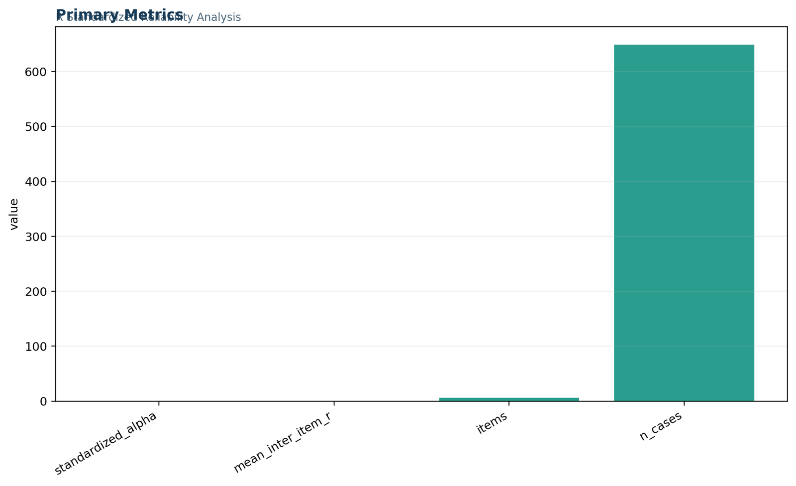
Figure 1. Primary reliability metrics
The chart summarizes standardized alpha 0.168910, mean inter-item correlation 0.032763, six items and 649 complete cases. The n-cases bar dominates because all four quantities share one axis. Read the coefficient labels numerically rather than judging their importance from bar height alone.
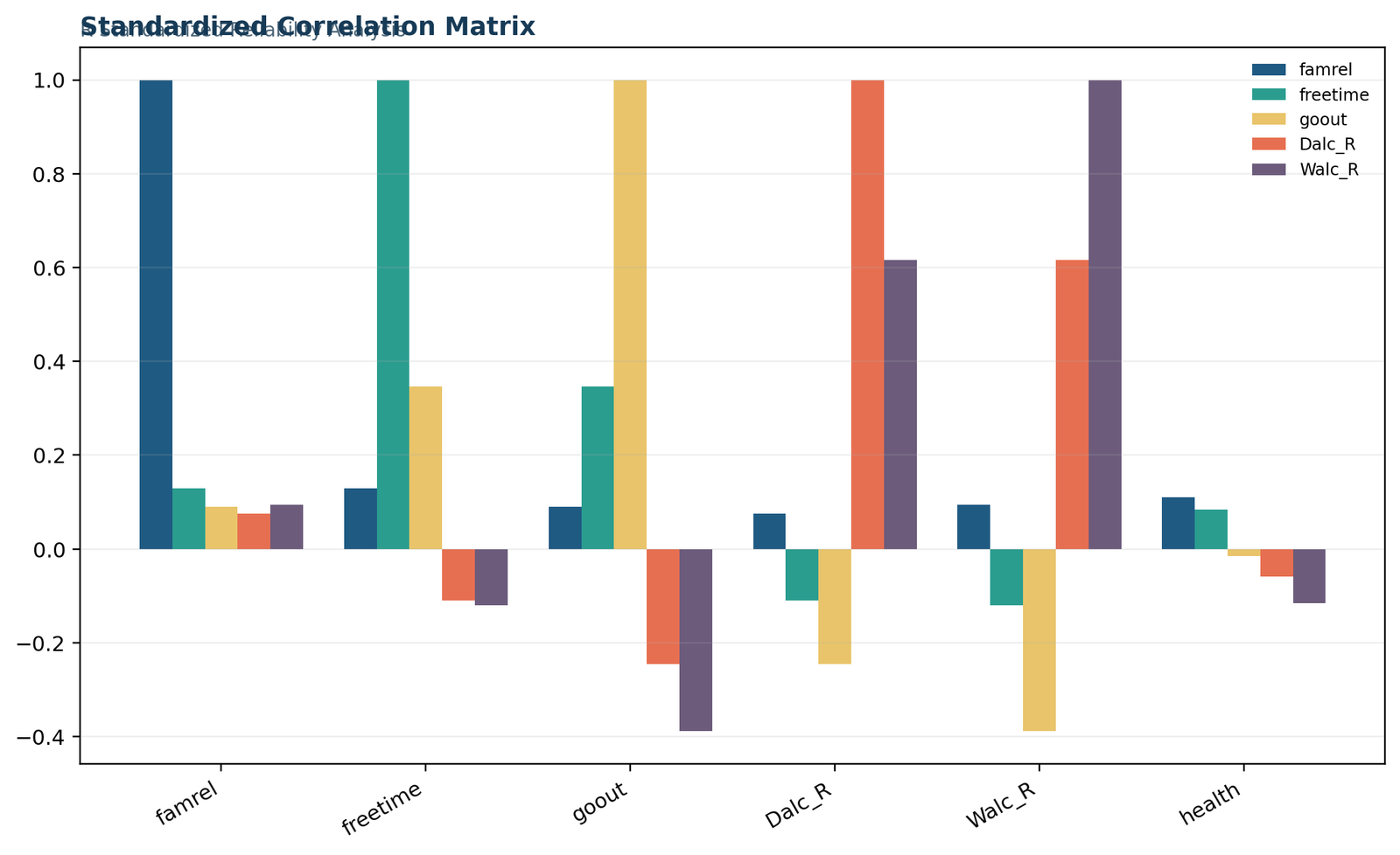
Figure 2. Standardized correlation matrix
The diagonal equals 1.00. The strongest off-diagonal positive relationship is Dalc_R with Walc_R at 0.617. Freetime with goout is 0.346. The largest negative relationship is goout with Walc_R at -0.389, followed by goout with Dalc_R at -0.245.
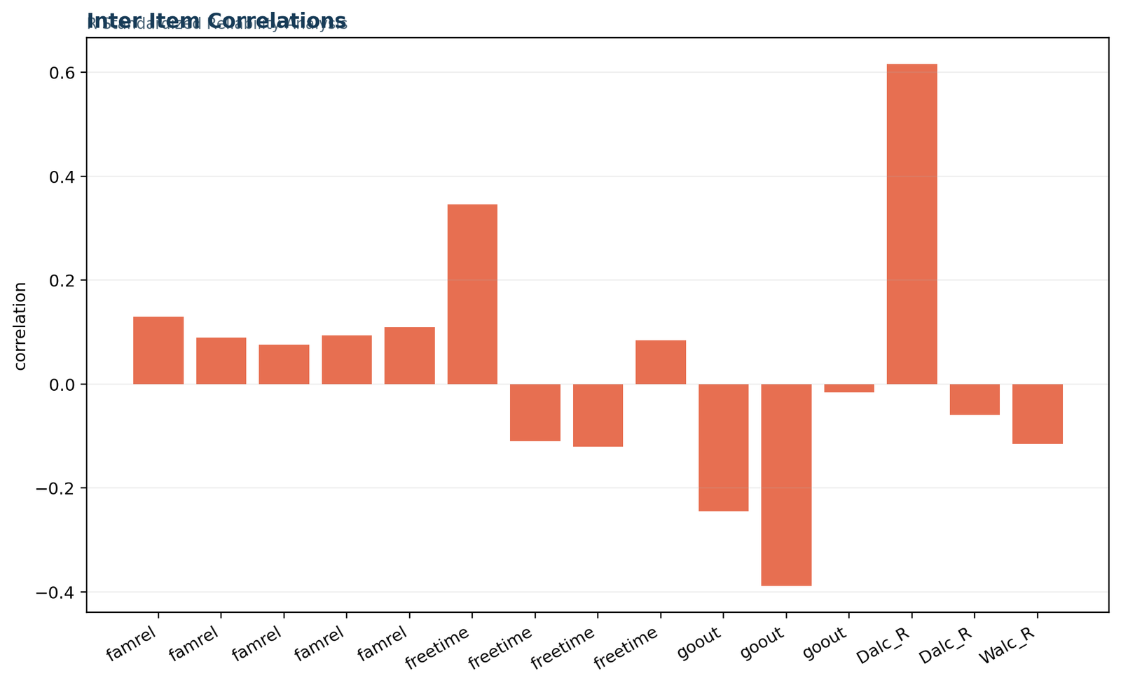
Figure 3. Unique inter-item correlations
The 15 bars are the upper-triangle values averaged to obtain r̄. Positive and negative associations visibly cancel. The concentration of small bars near zero explains why the mean is only 0.032763 even though two pairs are moderately or strongly positive.
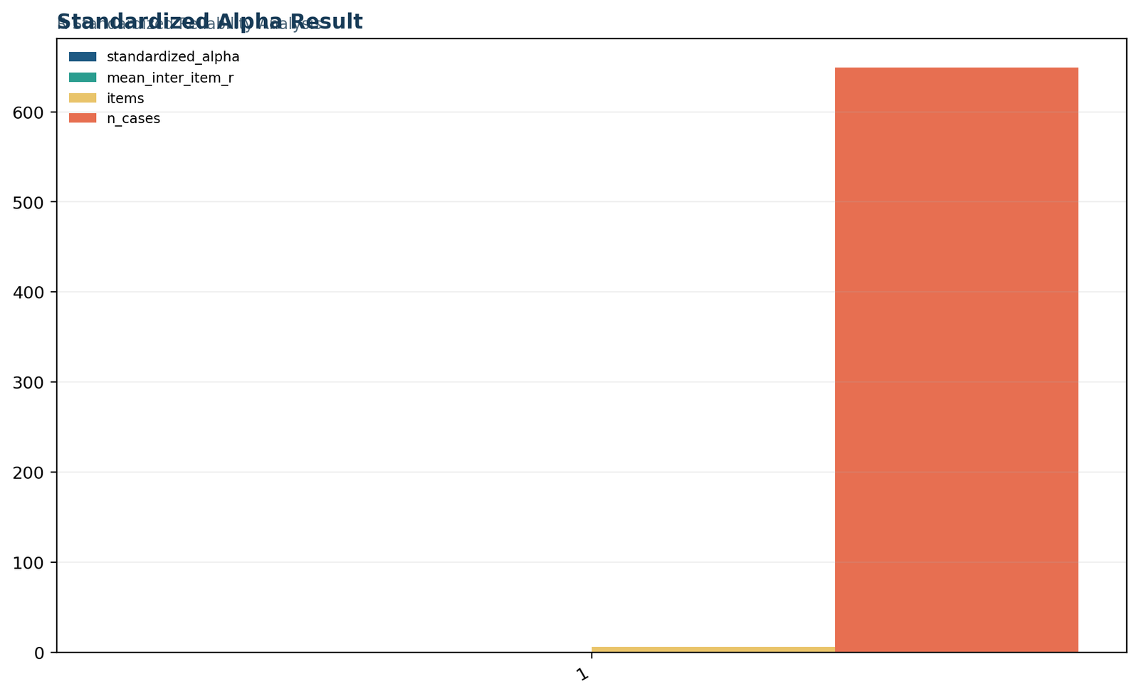
Figure 4. Standardized alpha result
On a focused coefficient scale, standardized alpha 0.168910 is clearly larger than the average correlation 0.032763 because the six-item formula accumulates shared information. The coefficient remains low because the average pairwise association is close to zero.
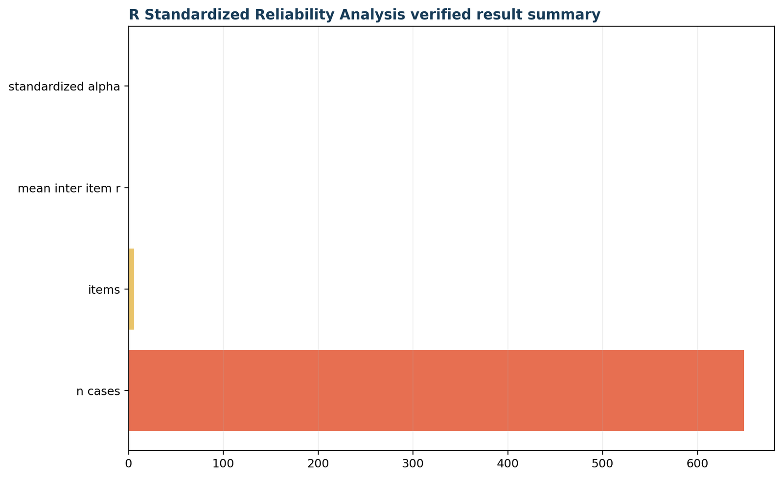
Figure 5. Verified R result summary
The final horizontal display confirms the same four values. It is a verification chart, not a new model. Agreement across the R report, formula substitution and figures supports computational reproducibility.
Detailed interpretation of Figure 1
Figure 1 is useful for verifying that the expected sample and item count entered the analysis. If the chart showed fewer than 649 cases, the missing-data filter or dataset selection would require investigation. If it showed more or fewer than six items, a column-selection error would be likely. In reliability analysis in R, these structural checks are as important as the coefficient because an accurate formula applied to the wrong rows or columns still produces an invalid answer.
The chart should not be used to compare the magnitude of n-cases with alpha. Cases are a count, items are a count, and the other two metrics are coefficients. Sharing one axis makes the small values almost invisible. The design works as a compact audit but not as a substantive comparison. The focused Figure 4 therefore supplies the coefficient-scale view.
Detailed interpretation of Figures 2 and 3
Figure 2 preserves item identity and reveals local structure. The family-relationship item correlates positively but weakly with every other item: 0.129 with freetime, 0.090 with goout, 0.076 with Dalc_R, 0.094 with Walc_R and 0.110 with health. Those values suggest broad favorable alignment, but none is large enough to establish a strong common factor.
Freetime correlates 0.346 with goout, indicating that students reporting more free time also tend to report more social outings. Its relationships with Dalc_R (-0.110) and Walc_R (-0.120) are negative after alcohol reversal, while its relationship with health is 0.085. The social-activity pair therefore behaves coherently with itself but not uniformly with the regulation items.
Goout has the most consequential negative cross-domain relationships: -0.245 with Dalc_R and -0.389 with Walc_R. Since higher reversed scores mean lower consumption, these signs indicate that more outings are associated with greater alcohol consumption. This relationship is substantively interpretable, but it lowers alpha because the proposed scale expects all high values to move together.
Dalc_R and Walc_R correlate 0.617, the largest off-diagonal value in the matrix. This pair likely forms a coherent alcohol-regulation subscale. Their correlations with health are -0.059 and -0.115, respectively, which are small and negative in this sample. Health itself correlates only 0.110 with famrel, 0.085 with freetime and -0.016 with goout. The health item is therefore not strongly integrated with either local cluster.
Figure 3 removes the diagonal and plots the exact 15 values that determine r̄. The order of bars follows the matrix extraction sequence rather than a ranked list, so interpretation should use the correlation table below. Its main visual message is heterogeneity: one strong positive bar, one moderate positive bar, several small positives, several small negatives and two notable negatives. A single coefficient cannot display that pattern.
Detailed interpretation of Figures 4 and 5
Figure 4 places standardized alpha and mean inter-item correlation on a shared coefficient scale. Standardized alpha is mathematically larger because it represents the reliability of a six-item aggregate rather than one average pair. The transformation is nonlinear: multiplying r̄ by six increases the numerator, while the denominator adjusts for repeated shared correlation. The exact result matches the formula section.
Figure 5 verifies the complete summary. It again places counts and coefficients together, so the 649-case bar dominates. The purpose is recordkeeping: confirm sample size, item count and coefficient values. In a published reliability analysis in R, the figure should be accompanied by text, as it is here, so small coefficients are accessible and not visually lost.
Exact standardized correlation matrix
The full matrix explains the low coefficient and identifies two local item clusters.
The exact matrix is the central diagnostic in this reliability analysis in R. Values are rounded to three decimals for display, while the coefficient was calculated from full-precision correlations. The diagonal is excluded from the average inter-item correlation.
| Item | famrel | freetime | goout | Dalc_R | Walc_R | health |
|---|---|---|---|---|---|---|
| famrel | 1.000 | 0.129 | 0.090 | 0.076 | 0.094 | 0.110 |
| freetime | 0.129 | 1.000 | 0.346 | -0.110 | -0.120 | 0.085 |
| goout | 0.090 | 0.346 | 1.000 | -0.245 | -0.389 | -0.016 |
| Dalc_R | 0.076 | -0.110 | -0.245 | 1.000 | 0.617 | -0.059 |
| Walc_R | 0.094 | -0.120 | -0.389 | 0.617 | 1.000 | -0.115 |
| health | 0.110 | 0.085 | -0.016 | -0.059 | -0.115 | 1.000 |
| Pair | Correlation | Contribution to reliability interpretation |
|---|---|---|
| famrel – freetime | 0.129 | Small favorable association. |
| famrel – goout | 0.090 | Very small positive association. |
| famrel – Dalc_R | 0.076 | Very small positive association with lower workday use. |
| famrel – Walc_R | 0.094 | Very small positive association with lower weekend use. |
| famrel – health | 0.110 | Small positive relationship. |
| freetime – goout | 0.346 | Moderate social-activity cluster. |
| freetime – Dalc_R | -0.110 | Small inverse cross-domain relationship. |
| freetime – Walc_R | -0.120 | Small inverse cross-domain relationship. |
| freetime – health | 0.085 | Very small positive relationship. |
| goout – Dalc_R | -0.245 | More outings align with higher workday consumption. |
| goout – Walc_R | -0.389 | Largest negative pair; more outings align with higher weekend consumption. |
| goout – health | -0.016 | Essentially no linear association. |
| Dalc_R – Walc_R | 0.617 | Strong alcohol-regulation cluster. |
| Dalc_R – health | -0.059 | Very small negative relationship. |
| Walc_R – health | -0.115 | Small negative relationship. |
The average of the full-precision values is 0.0327632893. The rounded table averages to a slightly different value because each cell has been shortened to three decimals. Always calculate reliability analysis in R from unrounded data and round only for presentation.
Cluster 1: social activity
Freetime and goout correlate 0.346, suggesting a coherent but only two-item social-activity component. A two-item scale requires special care because alpha is determined entirely by one correlation. The Spearman-Brown coefficient or direct reporting of the pair correlation may be clearer.
Family relations and health do not join this cluster strongly. Adding them to a social-activity score would broaden the construct and reduce homogeneity.
Cluster 2: lower alcohol use
Dalc_R and Walc_R correlate 0.617, indicating substantial consistency between lower workday and lower weekend alcohol use. These two variables have matching content and response format. A focused subscale would therefore be more coherent than the six-item total.
However, workday and weekend behavior are not identical. Report both the pair correlation and the rationale for combining them.
The matrix also illustrates why deleting negative items mechanically can be misleading. Removing goout would eliminate the two largest negative correlations and increase alpha, but it would also remove a central social-behavior variable. The correct decision depends on whether the intended construct is “self-regulation,” “wellbeing,” “social lifestyle,” or something else. Reliability analysis in R informs that decision; it does not define the construct automatically.
Diagnostics for reliability analysis in R
Alpha should be accompanied by dimensional, item-total, distribution and sensitivity checks.
A complete reliability analysis in R does more than print alpha. It examines whether one-factor interpretation is plausible, whether every item contributes in the intended direction, whether the coefficient depends on one influential item, and whether the result changes under reasonable correlation or missing-data choices.
Corrected item-total correlations
Each item should be correlated with the total of the remaining items, not with a total that includes itself. Including the item creates part-whole inflation. Low or negative corrected item-total correlations indicate that the item is weakly aligned with the rest of the proposed scale.
Use these correlations as diagnostic evidence, not automatic deletion rules. An item may be essential for content validity even when it lowers homogeneity.
Alpha if item deleted
This statistic recalculates alpha after removing one item. If deletion raises alpha, the item is reducing average consistency. Yet the gain may be trivial, and repeated deletion can produce a narrow, redundant scale that no longer covers the intended construct.
Document the original model, deletion rationale, revised coefficient and content consequences.
Dimensionality
Alpha does not establish one dimension. Inspect the matrix, scree plot, parallel analysis and factor loadings. The two visible clusters in this example suggest that a one-factor model is questionable. A McDonald’s omega analysis under a defensible factor model can provide a complementary coefficient.
Residual and local dependence checks
Items with nearly identical wording can share residual variance beyond the intended construct. This can inflate alpha. Conversely, items that measure different facets can reduce alpha. Examine content overlap and residual correlations rather than interpreting the coefficient in isolation.
Confidence intervals and sampling uncertainty
A point estimate does not show how precisely reliability is estimated. Bootstrap confidence intervals can be calculated by resampling respondents, recomputing the coefficient and taking percentile or bias-corrected limits. With 649 cases, the interval may be narrow, but it should still be reported when precision matters. See the internal confidence interval guide for general interpretation.
alpha_std <- function(z) {
R <- cor(z, use = "complete.obs")
rbar <- mean(R[upper.tri(R)])
k <- ncol(z)
(k * rbar) / (1 + (k - 1) * rbar)
}set.seed(20260728)
B <- 2000
boot_alpha <- replicate(B, {
index <- sample.int(nrow(x_complete), replace = TRUE)
alpha_std(x_complete[index, , drop = FALSE])
})
quantile(boot_alpha, c(0.025, 0.50, 0.975), na.rm = TRUE)
The bootstrap should resample rows because respondents are the independent units. Resampling individual cells would destroy the inter-item relationships that reliability analysis is designed to estimate. Report the bootstrap method, number of replications and random seed.
Ordinal sensitivity analysis
Five-category items can be analyzed with Pearson correlations, but an ordinal sensitivity analysis may be useful when categories are strongly skewed or treated as thresholds on latent continuous responses. A polychoric-based coefficient may differ because it estimates latent associations. Do not switch correlation types silently. State which matrix was used and why.
Missing-data sensitivity
The verified analysis uses 649 complete records. If another dataset contains missing items, compare listwise deletion with a principled model or imputation strategy. Pairwise correlations can use different sample sizes, while single imputation can overstate precision. A robust reliability analysis in R reports the missingness pattern, rule and final sample.
How to improve a weak reliability analysis in R result
Improve the measurement model, not merely the displayed coefficient.
When reliability analysis in R produces alpha 0.168910, the immediate task is to identify why the items do not cohere. The answer may be incorrect direction, poor wording, too few items, restricted variation, mixed dimensions, unsuitable respondents or a formative index. Each cause requires a different remedy.
Possible theory-based restructuring for the six items
Family and health context
famrel and health have a small positive correlation of 0.110. Two items are not enough to represent a broad wellbeing domain convincingly, but the pair can motivate development of additional family-support and health-perception items.
Social activity
freetime and goout correlate 0.346. This pair may represent opportunity for social activity, although more free time and more outings are not necessarily favorable or unfavorable. Define the construct without imposing a moral direction that the items do not support.
Alcohol regulation
Dalc_R and Walc_R correlate 0.617 and clearly share content. A focused lower-consumption score may be defensible, subject to the purpose and age-appropriate ethical context. The two original behavior indicators should also remain available separately.
Splitting the item set after seeing the matrix is exploratory. A new reliability analysis in R should be conducted on a validation sample or with cross-validation where feasible. Otherwise, the same random relationships that suggested the subscale also determine its reported coefficient, creating optimistic bias.
Adding items can increase reliability, but only if they correlate positively with the same construct. The Spearman-Brown prophecy formula estimates how scale length affects reliability under the strong assumption that new items have similar quality. With an average inter-item correlation of 0.032763, an impractically large number of comparable items would be needed for a high coefficient. This is further evidence that the item set requires conceptual restructuring rather than simple lengthening.
Improvement should also consider validity. Removing goout may increase alpha because it eliminates negative relationships with reversed alcohol variables, but the revised score may no longer represent social life. A narrow reliable scale is not automatically better than a broad transparent profile. Report component scores when the construct is intentionally multidimensional.
Reliability analysis in R compared with related coefficients
Different reliability and agreement statistics correspond to different measurement models and designs.
| Statistic | Main question | When it is preferable | Relationship to this example |
|---|---|---|---|
| Cronbach alpha | How consistently do items form a scale under an essentially tau-equivalent model? | Standard internal-consistency summary with item diagnostics. | The standardized form equals 0.168910. |
| McDonald’s omega | How much composite-score variance is attributable to common factors? | When a plausible factor model allows unequal loadings. | Useful only after dimensionality is modeled defensibly. |
| Guttman’s lambda | What lower-bound reliability estimates arise from alternative decompositions? | For complementary lower-bound analysis. | Does not solve mixed-dimensional content. |
| Split-half reliability | How consistent are two halves of a test? | When a meaningful split is defined and corrected for length. | Results depend on the chosen split. |
| Spearman-Brown coefficient | How does reliability change with test length or two-part consistency? | For length planning and two-item scales. | Relevant to the two-item local clusters. |
| Intraclass correlation coefficient | How reliable or agreeing are quantitative ratings or repeated measures? | For rater agreement, test-retest or clustered measurements. | Not a substitute for item internal consistency. |
| Cohen’s kappa | Do two raters agree on categories beyond chance? | For categorical classifications. | Not appropriate for six scored questionnaire items. |
| Fleiss kappa | Do several raters agree on nominal categories? | For multi-rater categorical designs. | Addresses agreement rather than scale consistency. |
A strong reliability analysis in R names the measurement model rather than selecting whichever coefficient is highest. Alpha, omega and lambda are not competing software scores. They estimate related but distinct quantities under different assumptions. If the item set is multidimensional, every one-number summary can be misleading unless the dimensions are modeled.
Alpha and omega
Alpha assumes a particular relationship among item true scores and errors. Omega uses factor loadings and can accommodate congeneric items. Omega is often preferred when one common factor is plausible but loadings differ. However, fitting a one-factor omega to a matrix with clear opposing clusters does not automatically create a valid unidimensional scale.
Use factor diagnostics first and explain the model. A higher omega than alpha is not proof that the scale is good.
Reliability and agreement
Internal consistency concerns different items administered within one occasion. Agreement coefficients concern judges or repeated measurements of the same target. The data layout may look similar, but the source of variation and intended generalization differ. Selecting the correct method requires identifying items, respondents, raters, occasions and targets explicitly.
Use the site’s agreement guides when the columns are raters rather than scale items.
How to report reliability analysis in R
A complete report names the items, scoring direction, sample, coefficient, matrix summary and interpretation.
Reporting reliability analysis in R requires more than writing “Cronbach’s alpha was low.” Readers need to know which items entered the scale, whether any were reversed, how missing values were handled, whether raw or standardized alpha was used, and what the coefficient implies for the proposed score.
APA-style worked example
A standardized internal-consistency analysis was conducted in R for six student-life items: family relationship quality (famrel), free time after school (freetime), going out with friends (goout), reverse-scored workday alcohol consumption (Dalc_R), reverse-scored weekend alcohol consumption (Walc_R), and current health status (health). Complete-case analysis retained 649 students. The mean inter-item correlation was .033, producing a standardized Cronbach alpha of .169 for the six-item set. Pairwise correlations ranged from -.389 for goout with Walc_R to .617 for Dalc_R with Walc_R. The item set therefore showed weak overall internal consistency and a heterogeneous correlation pattern, indicating that a single unqualified total score was not well supported.
Reporting checklist
Language to avoid
Do not say that 16.9% of the scale is reliable, that alpha is a percentage of variance explained, or that reliability analysis proves validity. Do not describe the coefficient as statistically insignificant unless a formal inference procedure was conducted and reported. Do not claim that R “rejected” the scale.
Prefer direct language: “standardized alpha was .169,” “the mean inter-item correlation was .033,” and “the heterogeneous matrix did not support a homogeneous six-item total.”
Round consistently. Three decimals are adequate for narrative reporting, while six or more decimals may be retained in verification tables or machine-readable output. Include leading zeros only according to the relevant style guide; APA style often omits the zero for coefficients bounded by -1 and 1.
When a confidence interval is available, report it after alpha and name the estimation method. When item deletion or subscale restructuring is exploratory, label it explicitly and confirm the revised model on new data. A transparent reliability analysis in R distinguishes planned scoring from post hoc optimization.
Common reliability analysis in R mistakes
Most serious errors arise from scale definition and coding rather than arithmetic.
Including every numeric column
Automatic selection of all numeric variables can combine age, grades, absences, identifiers and questionnaire items. R will calculate a coefficient, but the result has no coherent measurement interpretation. Select columns from a documented scoring key.
Reversing from the wrong maximum
For a 1-to-5 item, reversal is 6 – x. Using 5 – x creates values from 0 to 4 and shifts the scale. For a 0-to-4 item, reversal is 4 – x. Always derive the constant from minimum + maximum.
Converting factors with as.numeric
Direct as.numeric(factor) returns internal level codes, not necessarily the printed values. Convert through character or import numeric columns correctly. Verify ranges after conversion.
Letting automatic keying define theory
Automated key checks can reverse items to maximize consistency. This is useful for detecting possible errors, but it can also hide conceptual opposition. Record the intended direction before analysis.
Reporting alpha alone
The matrix in this example contains both 0.617 and -0.389. Reporting only 0.169 loses the reason for the result. Include average correlation, item diagnostics and dimensional evidence.
Using 0.70 as a universal law
Thresholds depend on purpose, stakes, scale length and construct breadth. A coefficient below 0.70 is not automatically useless, and one above 0.70 is not automatically valid.
Deleting until alpha rises
Repeatedly removing items on the same sample capitalizes on chance and can damage content coverage. Every deletion needs substantive justification and external confirmation.
Confusing reliability with validity
Consistent items can measure the wrong concept. Validate content, factor structure and relationships with external criteria in addition to reliability analysis in R.
Another common mistake is to compare alpha values from different item counts without considering length. A 20-item scale has more opportunities to accumulate shared covariance than a four-item scale. Compare average inter-item correlations, content breadth and score precision, not alpha alone.
Researchers also sometimes standardize items merely because standardized alpha is larger. The choice should reflect scoring. If the final composite is the raw sum, raw alpha is directly aligned with that score. If items use different units or the intended score gives equal standardized weight, standardized alpha may be more relevant. Report both when the distinction is consequential.
Reproducible reliability analysis in R workflow
A production workflow preserves the data decisions, calculations, figures and session details.
A reproducible reliability analysis in R should run from a clean script without manual edits to intermediate values. The script should identify the dataset, validate required columns, create reversed variables, filter the analysis sample, calculate the matrix and coefficient, save outputs and record the environment.
dir.create("R_Output", showWarnings = FALSE, recursive = TRUE)write.csv(R,
"R_Output/standardized_correlation_matrix.csv",
row.names = TRUE)
summary_values <- data.frame(
metric = c("standardized_alpha", "mean_inter_item_r", "items", "n_cases"),
value = c(standardized_alpha, mean_inter_item_r, k, nrow(x_complete))
)
write.csv(summary_values,
"R_Output/reliability_summary.csv",
row.names = FALSE)
capture.output(sessionInfo(),
file = "R_Output/R_session_info.txt")
Version-control the script and keep raw data read-only. Derived variables should be created in code so their definitions remain visible. Saving the matrix allows later checks without rerunning the entire workflow, while session information records the R version, platform and attached packages.
Use explicit random seeds for bootstrap intervals. Avoid hard-coded local paths when a project-relative path is possible. Test the script on a clean session because objects left in the workspace can hide missing imports or outdated values. A trustworthy reliability analysis in R is one that another analyst can reproduce from the documented inputs.
Reliability analysis in R is most useful when this numerical verification is interpreted beside the item definitions, scoring direction and complete correlation pattern.
Reliability analysis in R report download
The R-only report contains the verified metrics and all five R figures.
R reliability analysis reportStandardized alpha, mean inter-item correlation, six-item matrix, 649-case summary and the complete R figure set.Open R report
R primary metrics figureThe main R summary image showing the sample, item count, average correlation and standardized alpha.Open R figure
R correlation matrix figureThe complete standardized six-item correlation matrix used to calculate the mean inter-item correlation.Open R matrix
R verified result summaryThe final R verification figure confirming the coefficient, formula inputs and substantive conclusion.Open R summary
The report supports verification of the worked reliability analysis in R. The numerical result page states the design, variables, formula, sample size and calculated metrics. Subsequent pages display the primary metrics, standardized correlation matrix, unique inter-item correlations, focused alpha comparison and verified result summary.
R reliability documentation and numerical verification
Use the item definitions, formula audit, saved matrix and reproducible R objects to verify every reported value.
A dependable reliability analysis in R should be verifiable without relying on a screenshot alone. The item list, reverse-scoring rules, complete-case sample, correlation matrix, mean inter-item correlation and standardized-alpha formula should all remain available in the script and saved output files.
Base R verification
The upper triangle of the six-item correlation matrix contains 15 unique coefficients. Averaging those values gives 0.0327632893. Substituting that mean and k = 6 into the standardized-alpha formula gives 0.1689095702.
Package verification
The psych::alpha() output should reproduce the standardized coefficient and average correlation when the same six columns, reverse coding, complete cases and check.keys = FALSE setting are used. Any difference should trigger a check of the analysis sample and scoring direction.
Saved evidence
Retain the R script, session information, correlation matrix, summary CSV files and R report. These records show exactly how the 649 complete observations produced the reported reliability result.
Frequently asked questions about reliability analysis in R
Detailed answers to calculation, interpretation, coding and reporting questions.
What is reliability analysis in R?
Reliability analysis in R is a reproducible workflow for evaluating whether multiple scored items behave consistently enough to support a composite score. R can calculate raw and standardized Cronbach alpha, mean inter-item correlation, corrected item-total correlations, alpha if an item is deleted, split-half coefficients, bootstrap intervals and factor-based reliability estimates.
How do I run reliability analysis in R without a package?
Select the item matrix, calculate cor(), extract the upper triangle, average the unique correlations and apply α = kr̄/[1 + (k – 1)r̄]. The base R code in this guide reproduces standardized alpha 0.1689095702 for six items and 649 complete cases.
Which R package is commonly used for reliability analysis?
The psych package is widely used because psych::alpha() returns raw alpha, standardized alpha, average correlation, corrected item-total statistics and alpha-if-deleted output. Package output should be verified against the scoring key and matrix, especially when automatic key checking is enabled.
What does standardized alpha 0.1689 mean?
It indicates weak internal consistency for the six standardized items in this sample. The coefficient is low because the average inter-item correlation is only 0.032763 and the matrix contains several negative cross-domain relationships. The result does not support treating all six items as one homogeneous scale without further theory and dimensional analysis.
Why is the mean inter-item correlation only 0.0328?
The 15 unique correlations include strong positive values, small positive values and negative values. Dalc_R with Walc_R is 0.617, while goout with Walc_R is -0.389. Positive and negative pairs cancel in the mean, producing r̄ = 0.032763.
Does a large sample make reliability high?
No. A larger sample can estimate reliability more precisely, but it does not mechanically increase alpha. The 649 cases make the matrix stable; the coefficient remains low because item relationships are weak and heterogeneous.
Should I reverse Dalc and Walc before reliability analysis in R?
Reverse them when the intended scale defines higher scores as lower alcohol consumption and other items use a favorable high-score direction. For original 1-to-5 coding, use Dalc_R = 6 – Dalc and Walc_R = 6 – Walc. Preserve the originals and document the transformation.
Can R automatically detect reverse-keyed items?
Some functions can suggest reversals from the correlation pattern. Automatic detection is diagnostic, not a replacement for the questionnaire key. An item can correlate negatively because it was miscoded, because it is intentionally reverse-worded, or because it measures a different construct.
Is standardized alpha better than raw alpha?
Neither is universally better. Raw alpha matches the covariance structure of the raw summed items. Standardized alpha gives each item variance one and is useful when scales or variances differ or when standardized weighting is intended. Report the form that matches the score and consider both when they differ.
Does alpha prove that the scale is one-dimensional?
No. Alpha can be high for multidimensional or redundant items, and it can be low for a broad but meaningful construct. Use factor analysis, residual patterns and content theory to evaluate dimensionality. The present matrix visibly suggests at least social-activity and alcohol-regulation clusters.
Should I delete goout because it has negative correlations?
Not automatically. Removing goout would likely raise alpha because it has negative relationships with Dalc_R and Walc_R, but it would also change the construct and remove social-activity content. Decide whether goout belongs conceptually, inspect subscales, and confirm any revision on new data.
What is a good mean inter-item correlation?
There is no universal interval for every construct. Focused scales often show moderate positive average correlations, while broad constructs can be lower. Very high averages may indicate redundant items. Interpret r̄ with item count, content breadth and the complete matrix.
Can two items form a reliable scale?
Two items can be summarized when they have clear shared content, but alpha is then determined by their single correlation. Report the correlation and a Spearman-Brown coefficient, explain content coverage and recognize that two items provide limited diagnostic information.
How should missing items be handled?
Choose and report a rule before analysis. Complete-case analysis uses the same respondents for every pair, as in this 649-case example. Pairwise deletion can vary the sample across correlations. For substantial missingness, use a principled model or imputation strategy and perform sensitivity analysis.
Can reliability analysis in R use ordinal correlations?
Yes. Polychoric correlations may be considered for ordered categories viewed as thresholds on latent continuous variables. The resulting coefficient estimates reliability for that latent-correlation model and can differ from Pearson-based standardized alpha. State the matrix type explicitly.
Should reliability analysis include a p-value?
Alpha is normally reported as an estimate, preferably with a confidence interval when precision matters. A p-value is not the main reliability criterion. The present output reports no formal alpha p-value, so the coefficient should be interpreted descriptively.
How many decimals should I report?
Three decimals are generally adequate in narrative reporting: α = .169 and mean r = .033. Retain full precision in saved calculations and verification files. Avoid implying more measurement precision than the instrument supports.
Why can alpha be low after reverse coding?
Reverse coding fixes direction only. It does not make conceptually different variables measure one factor. In this example, reversed alcohol items remain negatively related to going out and weakly related to health, so standardized alpha stays low.
What should be reported beside alpha?
Report the item set, scoring direction, sample size, missing-data rule, raw or standardized form, mean inter-item correlation, correlation range, corrected item-total diagnostics, dimensional evidence and a substantive conclusion about the proposed total score.
What is the main conclusion of this reliability analysis in R?
The six transformed items do not support a strongly homogeneous total. Standardized alpha is 0.168910 and average inter-item correlation is 0.032763. The matrix instead suggests distinct social-activity and alcohol-regulation components, with family relations and health only weakly connected.
Related reliability and measurement guides
Continue with item diagnostics, alternative reliability coefficients and agreement methods.