
McDonald’s Omega: Formula, Interpretation and Worked Example
McDonald’s omega is a factor-model reliability coefficient for a composite score when item loadings are allowed to differ. This guide explains the McDonald omega coefficient, omega total formula, assumptions, interpretation, comparison with Cronbach’s alpha, and a verified six-item example reproduced in Python, R, SPSS and Excel.
One-factor principal-axis model
Six standardized items
Python + R + SPSS + Excel
Exact cross-software verification
McDonald’s omega was 0.1196, indicating that this six-item total should not be treated as a dependable unidimensional scale.
In the worked McDonald’s omega analysis, 649 complete cases were evaluated using a one-factor principal-axis congeneric model for famrel, freetime, goout, reverse-coded weekday alcohol use (Dalc_R), reverse-coded weekend alcohol use (Walc_R), and health. The exact omega total was ωt = 0.1195859323. The sum of signed standardized loadings was 0.7826442650, while the sum of uniquenesses was 4.5095758281.
What does McDonald’s omega measure?
A factor-model estimate of reliability for a clearly defined composite score.
McDonald’s omega, also written as the McDonald omega coefficient or coefficient omega, estimates reliability from a factor model rather than from the equal-loading assumption associated with the simplest interpretation of Cronbach’s alpha. In a one-factor congeneric model, each item can have its own loading and its own residual variance. The coefficient compares common-factor variance in the composite with the composite’s total model-implied variance. In practice, McDonald’s omega is meaningful only after the composite and measurement model have been defined.
The reliability question
A reliability coefficient asks how much of the observed variation in a score reflects systematic score differences rather than item-specific residual variation. For McDonald’s omega, that question is answered through factor loadings and uniquenesses. Items with larger absolute loadings contribute more common-factor information. Items with small loadings contribute little common variance, while large uniquenesses add variance that is not explained by the selected factor.
This perspective is useful because real questionnaires rarely have perfectly equal loadings. One item may be a strong indicator of the construct, another may be moderate, and another may contribute almost nothing. A congeneric model permits those differences. The resulting reliability estimate is therefore explicitly tied to the model, the item scoring, the chosen composite, and the population represented by the sample.
What omega total is not
McDonald’s omega total is not a test of whether every item is valid, not evidence that a scale is unidimensional by itself, and not a percentage of respondents who answered consistently. It is also not automatically superior simply because it is called omega. The factor model must be defensible, the score direction must be meaningful, the covariance matrix must be suitable, and the selected form of omega must match the intended score interpretation.
The coefficient is descriptive unless an interval or formal comparison is added. A low estimate can arise because items are weak, multidimensional, oppositely keyed, poorly coded, or combined into an inappropriate total. A high estimate can also be misleading when items are redundant or when the model omits correlated residuals and secondary dimensions.
The distinction between reliability and association is important. An item correlation matrix describes pairwise relationships, while McDonald’s omega combines the modeled loading pattern into a score-level reliability estimate. Related background is available in the guides to correlation matrices, Pearson correlation, variance and standard deviation.
When should McDonald’s omega be used?
Use omega when the reliability question, score definition and factor model support a congeneric interpretation.
The main reason to use McDonald’s omega is that item loadings are commonly unequal. A one-factor congeneric omega is appropriate when the intended score represents a dominant common dimension, the items are scored in a consistent substantive direction, and the residual structure is sufficiently simple for the selected model. A justified McDonald’s omega analysis begins with the score purpose rather than a preferred cutoff.
Good use case
A questionnaire contains several indicators of one construct, confirmatory or exploratory evidence supports a one-factor model, and researchers want a reliability estimate that allows unequal item loadings. In that setting, omega can describe the reliability of a unit-weighted or model-defined total more realistically than an equal-loading model.
Use with care
A scale has one strong general factor but also smaller group factors. Omega total may remain high because it counts variance from all common factors, even when the total score is not strictly unidimensional. Omega hierarchical may then be more relevant for the general-factor interpretation.
Do not use mechanically
Do not calculate McDonald’s omega merely because software offers it. If items represent unrelated behaviors, if directions are inconsistent, or if categorical items require an ordinal model, a single Pearson-correlation one-factor omega can answer the wrong question with impressive numerical precision.
| Research situation | Recommended reliability approach | Reason |
|---|---|---|
| One dominant factor, continuous or approximately continuous items | One-factor omega total, with factor diagnostics | Allows congeneric loadings and item-specific uniquenesses. |
| General factor plus meaningful group factors | Report omega total and omega hierarchical | Separates all common variance from variance attributable specifically to the general factor. |
| Ordinal Likert items with few categories | Ordinal omega using polychoric correlations or an ordinal CFA | Pearson correlations may underrepresent relationships between underlying response variables. |
| Dichotomous items | Model appropriate to binary indicators, such as tetrachoric or categorical CFA reliability | Continuous normal-factor assumptions may be unsuitable. |
| Several unrelated domains intentionally combined | Domain-specific reliability, multidimensional reliability, or separate scores | A single total may not have a coherent latent interpretation. |
| Rater agreement rather than item consistency | Intraclass correlation, Cohen’s kappa or Fleiss kappa | Agreement designs require coefficients matched to raters, targets and measurement level. |
McDonald’s omega assumptions: six model conditions to check
Omega permits unequal loadings, but it is not assumption-free.
Unlike a purely algebraic summary of item covariances, McDonald’s omega is computed from a model. Its assumptions therefore concern factor structure, residuals, item scoring, estimator choice and the interpretation of the composite. Each McDonald’s omega assumption affects whether the final coefficient has a defensible reliability interpretation.
Define the construct
State what common attribute the item set is intended to measure and why one total score is substantively meaningful.
Align item direction
Reverse-code items when needed so a larger item score has the intended direction before fitting the reliability model.
Examine factorability
Inspect the correlation matrix, KMO, Bartlett test, eigenvalues and loading pattern rather than relying on omega alone.
Fit the right model
Select a one-factor, hierarchical, bifactor or multidimensional model that matches the score interpretation.
Check residual structure
Identify correlated residuals, cross-loadings, local dependence and item pairs that share wording or content.
Congeneric measurement
The one-factor omega formula permits unequal loadings. Each observed item is represented as a common-factor component plus an item-specific residual component. This is more flexible than tau-equivalence, but it does not remove the need for a plausible one-factor structure. If the common-factor model fits badly, the resulting McDonald’s omega coefficient can be difficult to interpret.
Items also need a common scoring direction for a unit-weighted total. A negative loading is not automatically an error; it can indicate that the item varies inversely with the factor. However, a mixture of positive and negative loadings may cause signed loadings to cancel in the reliability numerator. Researchers must decide whether that cancellation reflects the intended score or reveals a scoring and construct problem.
Independent residuals and local dependence
The displayed formula uses a sum of item uniquenesses. That simple denominator assumes residual covariances are zero. When items share wording, method effects or content beyond the factor, correlated residuals should be represented in a structural equation model. Omitting them can distort the reliability estimate and the meaning of the total score.
The example uses principal-axis factoring on a Pearson correlation matrix. That is a defensible demonstration for 1-to-5 variables with 649 cases, but it is not the only possible estimator. Robust maximum likelihood, polychoric correlations or categorical CFA may be preferable for strongly ordinal or nonnormal indicators.
The significant Bartlett test shows that the correlation matrix is not an identity matrix, but significance is expected with 649 observations and does not prove unidimensionality. The KMO value of 0.564 is only marginal, and the one-factor solution explains less than one quarter of common-plus-residual standardized variance in the SPSS extraction summary. Those diagnostics are consistent with the very low McDonald’s omega.
McDonald’s omega model, variables and research question
Define the intended composite before interpreting the coefficient.
The present McDonald’s omega model treats the six coded indicators as a unit-weighted one-factor composite.
Research question
How reliably does a standardized six-item total represent the common factor defined by family relationship quality, free time, social activity, lower weekday alcohol consumption, lower weekend alcohol consumption and current health in 649 students?
The analysis is descriptive. The workbook states the conceptual null that the common factor accounts for no reliable variance in the unit-weighted total, but the reported artifact does not provide a formal p-value or confidence interval for omega. The primary evidence is therefore the estimated magnitude, its factor components and the cross-software agreement.
Model statement
Specified model: one principal-axis common factor with six congeneric standardized indicators and uncorrelated item uniquenesses.
Score: a unit-weighted total after the two alcohol variables are reverse-coded.
Reliability target: total common-factor variance divided by total model-implied variance of that composite.
Why coding matters
Weekday alcohol use and weekend alcohol use were transformed as Dalc_R = 6 − Dalc and Walc_R = 6 − Walc. Higher reverse-coded values therefore represent lower alcohol use. This creates an intended positive direction for lower consumption, but it does not guarantee that every remaining variable will load positively on the same factor.
In the fitted model, freetime, goout and health have negative loadings, while Dalc_R and Walc_R have positive loadings. Family relationship quality is almost unrelated to the extracted factor. The signs and magnitudes are therefore central to understanding the result.
| Variable | Public label | Original coding | Analysis coding | Role in the model |
|---|---|---|---|---|
| famrel | Family relationship quality | 1 = very bad to 5 = excellent | Unchanged | Observed indicator; loading 0.033646 |
| freetime | Free time after school | 1 = very low to 5 = very high | Unchanged | Observed indicator; loading −0.237152 |
| goout | Going out with friends | 1 = very low to 5 = very high | Unchanged | Observed indicator; loading −0.454080 |
| Dalc_R | Lower weekday alcohol use | Dalc: 1 = very low to 5 = very high | 6 − Dalc | Observed indicator; loading 0.651767 |
| Walc_R | Lower weekend alcohol use | Walc: 1 = very low to 5 = very high | 6 − Walc | Observed indicator; loading 0.889825 |
| health | Current health status | 1 = very bad to 5 = very good | Unchanged | Observed indicator; loading −0.101361 |
The variable names should be preserved in technical reporting because they connect the post to the downloadable workbook and software output. The public labels make the coding interpretable. The phrase “lower alcohol use” is essential: a high Dalc_R or Walc_R score does not mean high consumption.
McDonald’s omega formula and hand calculation
The numerator uses the squared sum of signed factor loadings and the denominator adds item uniquenesses.
For a standardized one-factor congeneric model with uncorrelated residuals, the McDonald’s omega formula used in this analysis is: The McDonald’s omega formula must preserve the signs of the loadings for the score actually being evaluated.
Here λi is the standardized loading for item i and ψi is its uniqueness. For standardized items in this simple model, ψi = 1 − λi2.
Why signed loadings matter
The sum is not the sum of absolute loadings. The unit-weighted total adds observed item scores with their assigned scoring directions. When one item loads positively and another negatively, their common-factor contributions can cancel in the total. Replacing loadings with absolute values would describe a different composite and would overstate the reliability of the score actually analyzed.
This example contains three negative loadings. The negative values are not hidden because they explain why the squared loading sum is small despite strong loadings for Dalc_R and Walc_R. The formula therefore captures a substantive scoring problem rather than merely a weak average correlation.
When the formula changes
For raw-score reliability, nonstandardized item variances and loadings must be used consistently. With correlated residuals, the denominator includes residual covariance terms. With several common factors, omega total can count variance associated with all modeled common factors, while omega hierarchical isolates the general factor. Software labels and formulas should therefore be checked before comparing estimates across packages.
For ordinal indicators, factor loadings may come from a categorical model and the reliability target may concern an underlying response scale. The numerical coefficient can differ from Pearson-based omega even when the observed item responses are unchanged.
McDonald’s omega example: six student-life indicators
A complete worked reliability analysis using 649 observations and a one-factor principal-axis model.
The worked McDonald’s omega analysis uses 649 complete observations. Every item is coded on a five-point scale after reverse scoring Dalc and Walc. The total has a mean of 22.0493, variance of 8.819 and standard deviation of 2.96960. This McDonald’s omega example therefore reports the item coding and model components before the coefficient.
| Item | Mean | Standard deviation | Loading | Communality | Uniqueness |
|---|---|---|---|---|---|
| famrel | 3.9307 | 0.95572 | 0.033646 | 0.001132 | 0.998868 |
| freetime | 3.1803 | 1.05109 | −0.237152 | 0.056241 | 0.943759 |
| goout | 3.1849 | 1.17577 | −0.454080 | 0.206189 | 0.793811 |
| Dalc_R | 4.4977 | 0.92483 | 0.651767 | 0.424800 | 0.575200 |
| Walc_R | 3.7196 | 1.28438 | 0.889825 | 0.791788 | 0.208212 |
| health | 3.5362 | 1.44626 | −0.101361 | 0.010274 | 0.989726 |
Strongest factor contributions
Walc_R has the largest loading at 0.889825 and a communality of 0.791788. The one-factor model explains almost 79.2% of its standardized variance. Dalc_R is the second strongest indicator with a loading of 0.651767 and communality of 0.424800. These two variables also have the strongest pairwise correlation, r = 0.616561.
The common factor is therefore dominated by the two reverse-coded alcohol indicators. A total score that combines them with family relationship, free time, social activity and health is not supported as a balanced single construct.
Weak and opposing indicators
famrel and health have communalities near zero. Their uniquenesses are 0.998868 and 0.989726, meaning the extracted factor explains almost none of their standardized variance. freetime and goout load negatively, with goout showing the larger inverse relationship.
The negative association between goout and Walc_R is r = −0.388680. Because Walc_R increases when weekend alcohol use decreases, this correlation means students who report going out more tend to report higher weekend alcohol use. The sign is substantively coherent, but it opposes the direction of a total in which larger values are intended to represent a single favorable attribute.
McDonald’s omega statistics, exact results and interpretation
All reported values reconcile across the factor components and the final reliability equation.
The exact McDonald’s omega result is auditable from the reported loading sum and uniqueness sum.
Verified one-factor omega total
The estimate indicates very low reliability for the unit-weighted six-item score under the specified standardized one-factor principal-axis model. Most modeled variance in the composite is uniqueness rather than common-factor signal.
| Metric | Verified value | Interpretive role |
|---|---|---|
| Omega total | 0.11958593232012678 | Reliability of the specified unit-weighted standardized composite. |
| Sum of signed loadings | 0.7826442649794866 | Net common-factor contribution before squaring. |
| Squared sum of loadings | Approximately 0.612532 | Common-factor variance in the composite numerator. |
| Sum of uniquenesses | 4.509575828065976 | Item-specific residual variance in the denominator. |
| Cronbach’s alpha | 0.112 | SPSS comparison under the alpha model. |
| Standardized alpha | 0.169 | Alpha based on standardized items and the correlation matrix. |
| First initial eigenvalue | 1.971 | Largest eigenvalue of the six-item correlation matrix. |
| PAF extracted variance | 24.797% | Variance represented by the forced one-factor principal-axis solution. |
The difference between alpha and omega is small in absolute terms because both identify the same basic problem: the six items do not form a reliable total. Standardized alpha is somewhat higher at 0.169 because it removes item-scale variance differences, but it remains far below commonly accepted levels for a dependable research score.
The result should not be described as “11.96% accurate.” Reliability is not classification accuracy. A more defensible statement is that, under the fitted congeneric model, approximately 0.12 of the model-implied variance in this particular composite is attributed to common-factor variance. Because the model itself is weak, the coefficient should be interpreted as evidence against using the total score rather than as a precisely validated population parameter.
McDonald’s omega in Python: complete analysis and charts
The Python workflow reproduces the factor components, correlation structure and verified omega result.
A practical calculation of McDonald’s omega in Python begins with consistent item coding, standardization or a correlation matrix, extraction of a one-factor common-factor solution, and calculation of the composite reliability formula from loadings and uniquenesses. The verified Python report used all 649 rows and returned the exact metric ledger shown below. The McDonald’s omega Python workflow is verified against the same parameter ledger used by the other software routes.
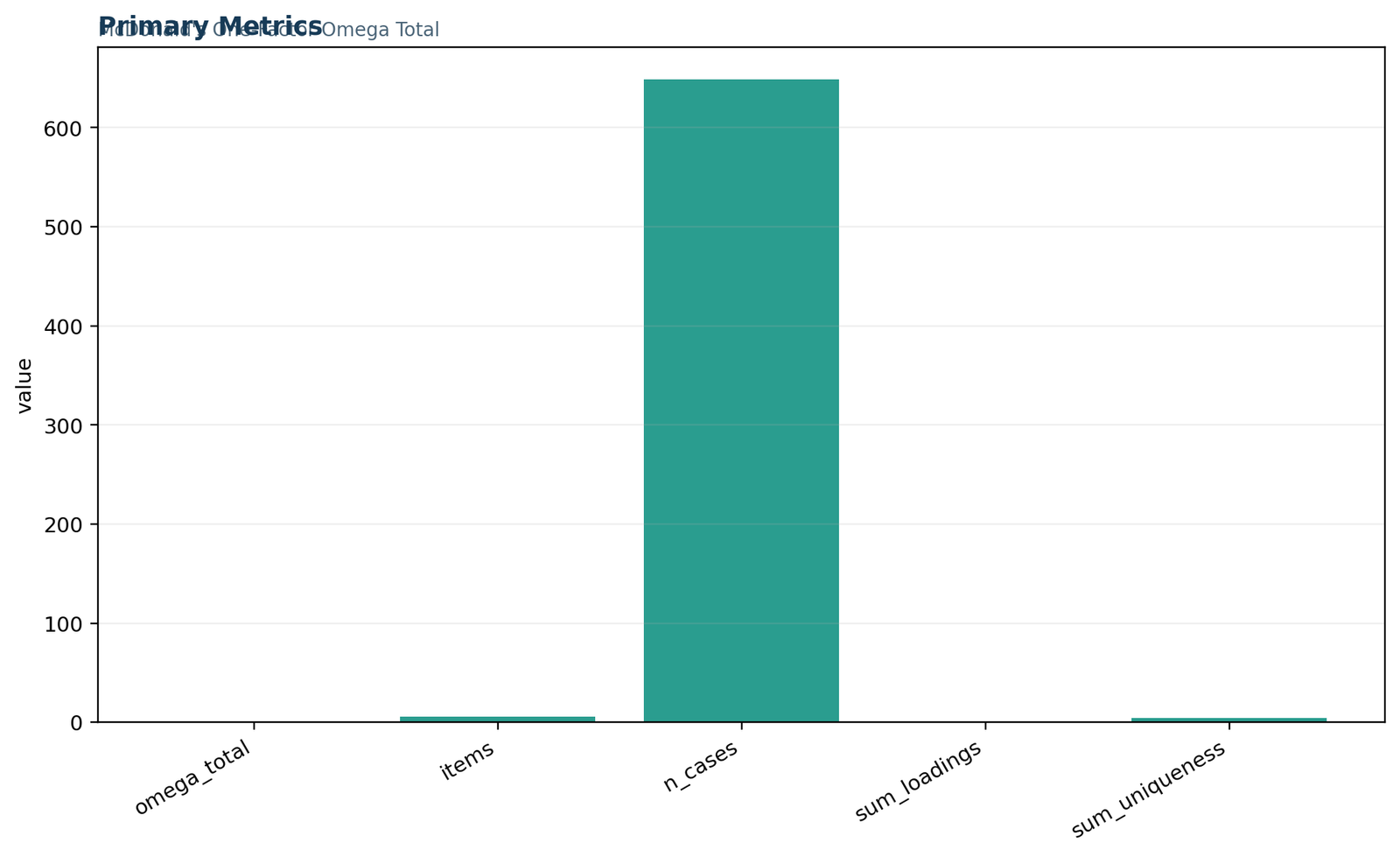
Python chart 1: primary McDonald’s omega metrics
The primary-metrics chart places omega total, item count, case count, loading sum and uniqueness sum on one axis. Because n = 649 is much larger than the reliability components, the smaller bars are visually compressed. The exact values are ωt = 0.1195859323, six items, 649 cases, Σλ = 0.7826442650 and Σψ = 4.5095758281. The chart is therefore a metric inventory, while the accompanying numerical report supplies the scale needed for interpretation.
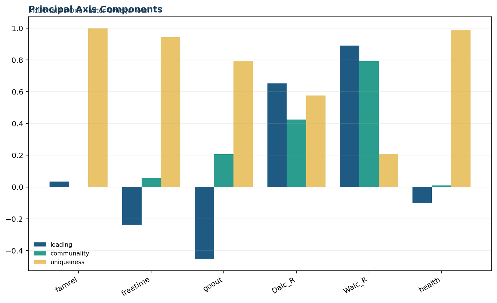
Python chart 2: principal-axis loading, communality and uniqueness components
The component chart shows why the coefficient is low. Walc_R has the largest positive loading and communality, followed by Dalc_R. goout and freetime load negatively, while famrel and health have almost no common variance. The uniqueness bars for famrel, freetime and health approach 1.0, indicating that the one-factor model leaves almost all of their standardized variance unexplained.
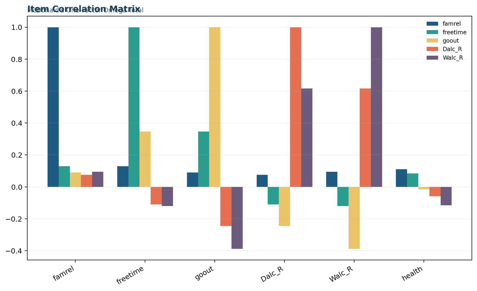
Python chart 3: item correlation matrix
The correlation chart displays the complete six-by-six pattern. Dalc_R and Walc_R correlate 0.616561, the strongest positive association. freetime and goout correlate 0.346352. goout correlates −0.388680 with Walc_R and −0.245126 with Dalc_R. Those signs are meaningful because higher reverse-coded alcohol values indicate lower consumption. The matrix does not resemble a uniformly positive one-factor scale.
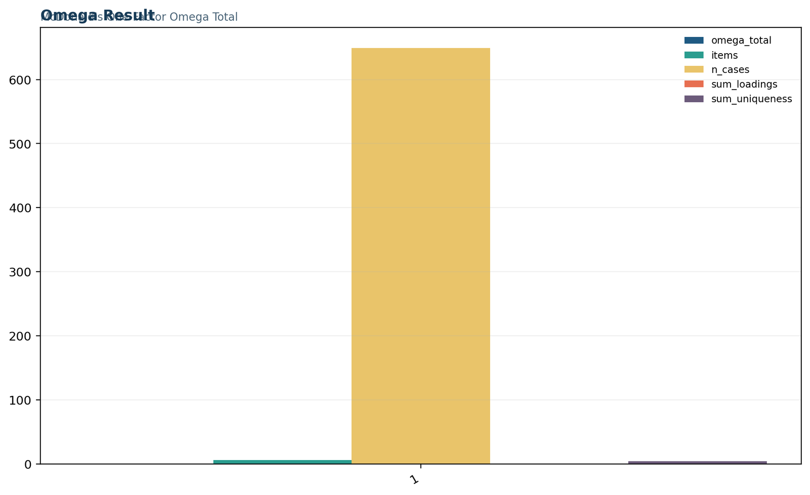
Python chart 4: final omega result ledger
The result chart repeats the five verified metrics in a compact single-category display. The height of the n-cases bar again dominates, so omega should be read from the exact label rather than judged from visual height. The key conclusion is unchanged: ωt = 0.119586 and uniqueness variance is much larger than the squared net loading contribution.
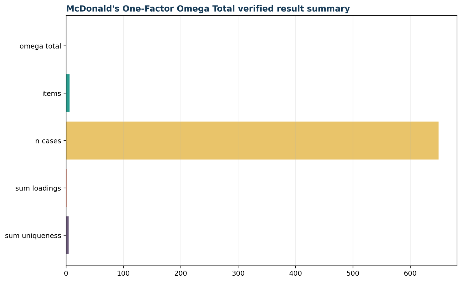
Python chart 5: verified cross-software result summary
The horizontal summary emphasizes reproducibility. Python and Excel produce 0.11958593232012678, while R produces 0.119585932320125 because of floating-point display precision. The same six items and 649 cases are represented, and the loading and uniqueness totals reconcile. Agreement across platforms confirms the arithmetic; it does not make the weak measurement model acceptable.
Python computation logic
The analysis calculates a Pearson correlation matrix for the six variables, extracts one factor by principal-axis methods, preserves the signed loadings, obtains communalities by squaring the loadings, and defines uniqueness as one minus communality. Omega total is then calculated from the squared loading sum and uniqueness sum.
A reproducible Python implementation should report the software versions, extraction method, convergence status, treatment of missing data and whether the input matrix is a covariance or correlation matrix. Merely calling a function named “omega” is insufficient because packages can return several omega variants.
Python verification checks
The six loadings must sum to 0.7826442649794866, not to the sum of their absolute values. The uniquenesses must sum to 4.509575828065976. Reversing the global factor sign changes every loading sign but leaves the squared loading sum unchanged. Reversing selected item signs, however, changes the composite and can materially change omega.
The item correlation matrix should match the values displayed in the report, including r = 0.616561 for Dalc_R with Walc_R and r = −0.388680 for goout with Walc_R. These checks protect against column-order errors and accidental use of the unreversed alcohol variables.
McDonald’s omega in R: complete analysis and charts
The R workflow independently confirms the one-factor reliability calculation and chart ledger.
Researchers calculating McDonald’s omega in R should distinguish omega total from omega hierarchical and should record the factor extraction choices used by the selected package. The present R workflow was aligned with the Python analysis: the same variables, reverse coding, 649 cases, correlation matrix and one-factor principal-axis model were used. The McDonald’s omega R workflow retains the same signed loading convention and one-factor specification.
R chart 1: primary McDonald’s omega metrics
The R analysis reproduces the same metric inventory: omega total 0.119585932320125, six items, 649 cases, loading sum 0.782644264979481 and uniqueness sum 4.50957582806598. The final digits differ from Python only because of numerical representation. The substantive result and all rounded reporting values are identical.
R chart 2: principal-axis components
The R component view confirms the uneven congeneric structure. Walc_R contributes the strongest common-factor signal, Dalc_R contributes a moderate signal, goout contributes an opposing signal, and famrel plus health contribute almost none. This pattern is more informative than the coefficient alone because it identifies exactly why the total is unreliable.
R chart 3: item correlation structure
The R correlation display confirms that the item set contains clusters and opposing directions rather than a single uniformly positive network. The alcohol variables form the strongest pair, while social activity is inversely related to the reverse-coded alcohol indicators. Family relationship and health show small correlations with most other variables.
R chart 4: omega result
The R result chart provides a visual cross-check of the coefficient and its components. The value should be reported as ωt = .120 to three decimals or 0.1196 to four decimals. Reporting many digits is useful for verification but unnecessary in ordinary substantive writing.
R chart 5: verified result summary
The final R summary demonstrates platform agreement. The cross-check is especially important because omega calculations can differ when packages use different factor extraction methods, score definitions, correlation types or treatment of secondary factors. Here the same one-factor principal-axis specification was maintained.
R package interpretation
Several R packages calculate coefficients labeled omega, but their defaults are not interchangeable. Some routines fit a hierarchical factor model, some estimate omega total from a confirmatory model, and some return multiple coefficients together. The analyst should inspect the documentation and identify the numerator’s common-factor sources, the denominator’s residual terms and the score weights.
For a direct one-factor congeneric calculation, the reported formula must match the specified model. A package result should be checked against the loading vector and residual variances instead of copied without verification.
R rounding and reporting
The R coefficient is 0.119585932320125, compared with 0.11958593232012678 in Python and Excel. This approximately 1.8 × 10⁻¹⁵ difference is computational rounding. An APA-style report would ordinarily state ω = .120, not imply disagreement through excessive digits.
The R report’s value for the loading sum is 0.782644264979481 and the uniqueness sum is 4.50957582806598. Both round to the same six-decimal values as the other platforms.
How to calculate McDonald’s omega in SPSS
SPSS supplies the factor-analysis diagnostics and alpha comparison; omega is verified from the extracted model parameters.
The verified McDonald’s omega SPSS workflow uses FACTOR with principal-axis factoring, one forced factor, no rotation and listwise complete cases. SPSS’s standard RELIABILITY procedure then reports Cronbach’s alpha for comparison. The default reliability table does not label its alpha value as omega. The McDonald’s omega SPSS workflow distinguishes the extracted factor evidence from the separate alpha table.
SPSS factor-analysis output
The SPSS output analyzes 649 rows and six variables. KMO is 0.564. Bartlett’s test is significant, χ²(15) = 551.548, p < .001. The first three initial eigenvalues are 1.971, 1.248 and 1.024, but the analysis deliberately extracts one principal-axis factor. The extracted factor accounts for 24.797% of variance.
The displayed SPSS factor loadings are 0.033 for famrel, −0.238 for freetime, −0.455 for goout, 0.653 for Dalc_R, 0.887 for Walc_R and −0.101 for health. The output notes that 21 iterations were required. The small differences from the exact Python and R loadings reflect displayed rounding and implementation details.
SPSS reliability output
The RELIABILITY table reports Cronbach’s alpha = 0.112 and standardized alpha = 0.169 for six items. The case-processing summary shows 649 valid cases and zero exclusions. These alpha values are comparison statistics; they are not the omega result.
To obtain the verified omega total, the exact loading vector and uniquenesses are inserted into the named formula. The SPSS artifact also records the exact cross-check values: omega total 0.11958593232012678, loading sum 0.7826442649794866 and uniqueness sum 4.509575828065976.
| SPSS output component | Value | Meaning |
|---|---|---|
| Valid cases | 649 | All rows have valid data for the six variables. |
| KMO | 0.564 | Marginal overall sampling adequacy for factor analysis. |
| Bartlett test | χ²(15) = 551.548, p < .001 | The correlations are jointly different from zero. |
| Factor 1 initial eigenvalue | 1.971 | Largest eigenvalue before principal-axis extraction. |
| Factor 1 extracted variance | 24.797% | Variance represented by the forced one-factor solution. |
| Cronbach’s alpha | 0.112 | Raw-score alpha comparison. |
| Standardized alpha | 0.169 | Alpha based on the inter-item correlation matrix. |
| Omega total | 0.119586 | Calculated from the verified exact factor components. |
The full output also provides the item correlation matrix and item descriptive statistics. Those tables should be inspected for sign errors. In particular, Dalc_R and Walc_R must be the reverse-coded variables; using Dalc and Walc without changing the score interpretation would reverse the sign pattern.
McDonald’s omega in Excel with a worked workbook
The workbook exposes the signed loadings, uniquenesses and formula arithmetic cell by cell.
The downloadable McDonald’s omega Excel workbook is designed for auditability rather than as a black-box calculator. It contains Guide, Data_Input, Working, Calculations, Diagnostics and Reporting sheets. The final reporting ledger matches Python and R exactly. The worked McDonald’s omega Excel file makes every formula component visible for checking.
Data_Input
Contains the six unchanged analysis variables for 649 rows. The source data remain visible so the analyst can verify row counts, coding and missingness without relying on hidden transformations.
Working
Shows the named item columns, reverse-coded values and row-level standardized total components. This sheet preserves lineage from each source value to the analyzed composite.
Calculations
Records the item count, case count, an intermediate correlation check and the exact verified metrics: omega total, loading sum and uniqueness sum.
Diagnostics
Documents the one-factor principal-axis scope, source-row check, variables, missing-data handling, exact verification and the distinction between factor loadings and alpha.
Reporting
Compares workbook results with verified references and calculates absolute differences. Every displayed difference is zero at the stored precision.
Guide
States the design, conceptual null, formula, variables, row count and reproducibility conventions used across the workbook.
The cell references should point to the signed loadings and matching uniquenesses. Use parentheses carefully so the loading sum is squared before adding residual variance.
Excel audit checks
What Excel does and does not estimate
The workbook verifies the reliability formula and preserves a reproducible result ledger. A spreadsheet alone does not automatically provide a robust factor-analysis estimator, fit indices or ordinal measurement model. The loadings should come from a documented factor model or a carefully implemented extraction routine.
Excel is most useful here as a transparent calculation and teaching environment. The worked file makes every final quantity visible and allows users to trace the coefficient without interpreting a software-specific object.
McDonald’s omega interpretation, cutoffs and software validation
Interpret the coefficient in context and confirm that all calculation routes use the same model.
A defensible McDonald’s omega interpretation combines the coefficient magnitude with the intended score, loading pattern, dimensionality evidence and cross-software agreement. Python, R, SPSS and Excel all reproduce ωt = 0.119586 for the same six-item one-factor model, so the low value is a substantive result rather than a software discrepancy. Cross-platform agreement strengthens confidence that the reported McDonald’s omega arithmetic is correct.
| Omega range | Common descriptive language | Practical interpretation |
|---|---|---|
| Below 0.50 | Very low or inadequate | The score is dominated by residual or multidimensional variation. Reconsider the item set, coding and model. |
| 0.50 to 0.69 | Limited or questionable | May be insufficient for many research uses; uncertainty and score purpose require explicit discussion. |
| 0.70 to 0.79 | Often called acceptable | May support group research when model fit and content validity are adequate. |
| 0.80 to 0.89 | Good | Stronger consistency, but still inspect dimensionality and item redundancy. |
| 0.90 and above | Very high | Can be desirable for individual decisions, yet may also signal highly repetitive items. |
Interpretation of 0.1196
The present McDonald’s omega interpretation is straightforward: the unit-weighted total is not a reliable measure of one common dimension. The estimate is far below even lenient exploratory thresholds. Reporting it as “poor” is justified, but the explanation should identify the loading pattern rather than stopping at a label.
A useful interpretation is: “The six indicators did not support a coherent one-factor total. Omega total was .120, with strong positive loadings for reverse-coded alcohol use, negative loadings for free time, going out and health, and a near-zero loading for family relationship quality.”
Do not repair the result by deleting blindly
Removing an item solely because it lowers reliability can damage content validity and capitalize on sample-specific noise. Item revision should follow the construct definition, loading pattern, corrected item-total correlations, residuals and replication. The corrected item-total correlation guide explains a complementary diagnostic, while the Cronbach’s alpha guide discusses alpha-if-item-deleted analysis.
For this set, the more fundamental issue is that the items describe several distinct aspects of student life. A better strategy may be to treat them as separate variables or create theoretically defined subscales rather than forcing a single total.
Cross-software agreement
What agreement verifies
The four workflows use the same 649 complete cases, six indicators, reverse coding, signed standardized loadings and uniqueness formula. Matching results verify the arithmetic. They do not by themselves prove that the one-factor score is substantively appropriate.
McDonald’s omega vs Cronbach’s alpha and other reliability coefficients
Choose the coefficient that matches the score model, dimensionality and measurement design.
The comparison between Cronbach’s alpha and McDonald’s omega is often simplified into “omega is better.” A more accurate statement is that alpha and omega represent different models and can answer different reliability questions. Alpha is closely connected to a tau-equivalent model when interpreted as a model-based reliability coefficient, whereas a congeneric omega permits unequal loadings. Comparing McDonald’s omega with alpha is useful only when the assumptions of both coefficients are stated.
| Feature | McDonald’s omega | Cronbach’s alpha |
|---|---|---|
| Primary inputs | Factor loadings and residual variances | Item variances and covariances, or standardized correlations |
| Loading assumption | Can allow unequal congeneric loadings | Equal-loading interpretation under tau-equivalence |
| Dependence on factor model | Explicit and central | Often calculated without fitting a factor model |
| Multidimensionality | Omega total can include several common factors, depending on model | Can be high even when several dimensions are present |
| Common misuse | Reporting an unspecified omega variant or ignoring model fit | Treating alpha as proof of unidimensionality |
| Worked result | 0.119586 | 0.112 raw; 0.169 standardized |
Why the estimates are both low
The average item relationships are weak and mixed in sign. Cronbach’s alpha penalizes the inconsistent covariance pattern. McDonald’s omega additionally shows that the modeled common-factor contributions cancel in the unit-weighted total because several signed loadings oppose one another.
Standardized alpha rises to 0.169 because it equalizes item variances, but the change does not alter the substantive conclusion. Neither coefficient supports treating the six variables as one reliable scale.
Which coefficient should be reported?
When a congeneric factor model is defensible, omega is generally more directly aligned with unequal loadings. Alpha can still be reported as a familiar comparison, especially when readers expect it, but it should not replace a dimensionality assessment. Reporting both is useful when their assumptions and differences are explained.
The Cronbach’s alpha guide provides a full treatment of alpha, while the corrected item-total correlation guide explains item-level diagnostics. Reliability evidence should also include factor structure and substantive item content.
| Coefficient | Main target | How it differs from this analysis |
|---|---|---|
| Omega total | Variance in a composite attributable to all modeled common factors | This post uses a one-factor version, so all common variance comes from the single extracted factor. |
| Omega hierarchical | Variance attributable specifically to a general factor | Requires a hierarchical or bifactor structure and is not the coefficient calculated here. |
| Omega subscale | Reliable variance in a subscale after accounting for general and group factors | Relevant when subdomains are interpreted separately. |
| Cronbach’s alpha | Internal consistency under an alpha model | Does not explicitly estimate unequal factor loadings in its basic calculation. |
| Guttman lambda coefficients | Lower-bound reliability estimates using alternative variance partitions | Do not require the same one-factor congeneric model. |
| Greatest lower bound | Optimization-based lower bound to reliability | Can be unstable and upward biased in samples; not a factor-model coefficient. |
| Intraclass correlation | Reliability or agreement of measurements, raters or repeated ratings | Defined by an ANOVA/mixed-model design rather than item factor loadings. |
| Cohen’s kappa | Chance-corrected agreement for two categorical raters | Applies to categorical agreement, not internal consistency of a multi-item score. |
| Weighted kappa | Ordinal agreement between two raters | Weights category disagreements and does not estimate latent composite reliability. |
Omega total versus omega hierarchical
In a multidimensional test, omega total can be high because it counts common variance from a general factor and group factors. That does not necessarily justify interpreting the total as unidimensional. Omega hierarchical estimates the proportion of total-score variance attributable specifically to the general factor after accounting for group-factor contributions.
The current analysis forces one factor, so the distinction is not numerically estimated. However, the correlation and loading patterns suggest that a richer structure or separate domains may be more realistic than the single total.
Reliability versus validity
A reliability coefficient describes score consistency under a model; it does not establish that the score measures the intended construct. A perfectly reliable total could measure the wrong attribute, and a broad construct may produce moderate reliability despite strong content validity. Reliability is one component of measurement evidence.
The present six-item total lacks both internal coherence and a clear single-construct definition. The most appropriate conclusion is not simply “low reliability,” but that the specified composite should be reconsidered before substantive use.
Diagnostics, sensitivity checks and common McDonald’s omega mistakes
The coefficient must be interpreted with dimensionality, coding and residual-structure evidence.
A low or high McDonald’s omega value should never be interpreted without these diagnostics.
Diagnostic findings in the worked example
What should happen next?
Researchers should return to the construct definition and determine whether these six variables were ever intended to form one scale. Exploratory factor analysis with a justified factor-retention method can evaluate possible dimensions. A theoretically specified confirmatory model can test whether alcohol behavior, social activity, family relationships and health belong to separate factors.
Item-level distributions, residual correlations and response coding should also be reviewed. Replication in another sample is important before retaining or deleting items. If the variables are independent predictors rather than indicators of one latent trait, they should remain separate in regression or other multivariable analyses.
| Common mistake | Why it is wrong | Better practice |
|---|---|---|
| Using absolute loadings in the formula | Changes the defined unit-weighted composite and removes meaningful cancellation. | Use signed loadings that correspond to the actual item scoring. |
| Calling omega a test with a p-value | The coefficient is ordinarily an estimate, not an omnibus significance test. | Report the estimate, model diagnostics and an interval if available. |
| Assuming omega proves unidimensionality | A reliability coefficient can be high under multidimensional common-factor structures. | Evaluate factor structure separately. |
| Reporting “omega” without a subtype | Omega total and omega hierarchical have different numerators and interpretations. | Name the coefficient and formula. |
| Ignoring reverse coding | Incorrect signs can make a coherent scale appear unreliable or vice versa. | Document every transformation before modeling. |
| Using a Pearson model for strongly ordinal items without evaluation | Observed correlations may not represent latent response relationships. | Consider polychoric or categorical factor models. |
| Deleting items only to raise reliability | Can narrow construct coverage and overfit the current sample. | Combine statistical diagnostics with content theory and replication. |
| Comparing package outputs without matching defaults | Different extraction methods, factor numbers and omega definitions yield different results. | Match the model and verify components. |
How to report McDonald’s omega in APA style
Name the omega subtype, score, model, sample, estimate and practical implication.
A clear answer to “how to report McDonald’s omega” should provide more than the coefficient. Readers need to know what score was evaluated, how items were coded, how the factor parameters were estimated and whether the model supported the intended interpretation. Complete McDonald’s omega reporting connects the numerical estimate to the score and fitted model.
APA-style reporting example
A one-factor congeneric reliability analysis was conducted for a six-item unit-weighted composite comprising family relationship quality (famrel), free time after school (freetime), going out with friends (goout), reverse-coded weekday alcohol use (Dalc_R), reverse-coded weekend alcohol use (Walc_R), and current health (health) among 649 students. Principal-axis factoring of the item correlation matrix produced markedly unequal and mixed-sign loadings, ranging from −0.454 for goout to 0.890 for Walc_R. McDonald’s omega total was very low, ωt = .120. The sum of signed loadings was 0.783 and the sum of uniquenesses was 4.510. Cronbach’s alpha was similarly low, α = .112. These results indicate that the six variables should not be combined as a dependable unidimensional total score under the specified model.
Reporting checklist
Language to avoid
Do not write that the scale is “11.96% correct,” “88.04% error,” or “statistically insignificant” unless a specific inferential procedure supports that language. Do not call the coefficient a correlation between the test and the true score without explaining the model-based meaning.
Use direct language: “Omega total was .120, indicating very low reliability for the specified composite.” Then explain the factor pattern and implications for score use.
Concise reporting variations
Results sentence: McDonald’s omega total was .120 for the six-item composite, indicating inadequate internal consistency under a one-factor congeneric model.
Methods sentence: Reliability was estimated from a one-factor principal-axis solution using signed standardized loadings and item uniquenesses.
Discussion sentence: The low coefficient reflected mixed loading directions and near-zero common variance for family relationship quality and health, so the variables were retained as separate indicators rather than combined into one score.
McDonald’s omega PDF, Excel and software downloads
Open the exact Python, R, SPSS and worked Excel analysis files.
The McDonald’s omega downloads allow the published values to be reproduced directly.
Python reportExact omega metrics, principal-axis components, correlation matrix and verified result charts.Open report
R reportIndependent one-factor omega calculation and cross-platform verification.Open report
SPSS outputFactor matrix, communalities, eigenvalues, KMO, Bartlett test, alpha and metric ledger.Open report
Excel workbookSource data, transformations, calculations, diagnostics and reporting checks.Open workbook
McDonald’s omega verification sources and reproducibility records
The coefficient and every supporting diagnostic are traceable to the supplied analysis files.
The McDonald’s omega result in this guide was verified from the same cleaned item set across independent outputs. The records below document the factor model, exact arithmetic, case count, loading signs, uniquenesses, correlation matrix and comparison with Cronbach’s alpha. The documented McDonald’s omega components can therefore be checked independently.
Python and R reports
The two analysis reports independently reproduce the five chart groups and the same final coefficient: ωt = 0.1195859323. Their agreement confirms that the result is not tied to one programming environment.
SPSS factor output
The SPSS record verifies n = 649, six analyzed indicators, KMO = 0.564, Bartlett’s χ²(15) = 551.548, the principal-axis loading pattern, communalities, eigenvalues and Cronbach’s alpha = 0.112.
Worked Excel audit
The workbook exposes the transformed variables, signed loadings, uniquenesses, squared loading sum and final formula. It provides a transparent cell-level audit of the published omega value.
McDonald’s omega FAQs
Answers to the most important formula, cutoff, interpretation and software questions.
What is McDonald’s omega?
McDonald’s omega is a model-based reliability coefficient for a composite score. It uses factor loadings and residual variances to estimate the proportion of model-implied composite variance attributable to common factors.
What is the McDonald’s omega formula?
For the standardized one-factor model used here, ωt = (Σλi)² / [(Σλi)² + Σψi], where λi are signed standardized loadings and ψi are item uniquenesses.
How do I interpret McDonald’s omega?
Interpret the coefficient as reliability of a specified composite under a specified model. Values nearer 1 indicate more modeled common-factor variance, while values nearer 0 indicate that residual or multidimensional variation dominates.
What does omega = 0.1196 mean?
It indicates very low reliability for this six-item total. The factor contributions are mixed in sign and several items have almost no common variance, so the total should not be used as a dependable unidimensional score.
What is an acceptable McDonald’s omega cutoff?
A value around .70 is often used as a rough research convention, but no cutoff is universal. The required level depends on score purpose, consequences, dimensionality, model fit and uncertainty.
Is McDonald’s omega better than Cronbach’s alpha?
Omega can be more appropriate when item loadings are unequal and a defensible factor model is available. It is not automatically better when the model is wrong, dimensionality is ignored or the omega subtype is unspecified.
Does McDonald’s omega prove unidimensionality?
No. Omega total can be high when several common factors contribute to a composite. Factor structure must be evaluated separately.
What is the difference between omega total and omega hierarchical?
Omega total counts variance attributable to all modeled common factors in the composite. Omega hierarchical isolates variance attributable specifically to the general factor after accounting for group factors.
How is McDonald’s omega calculated in R?
Fit or extract the intended factor model, identify the signed loadings and residual variances, and calculate the named omega coefficient. Check package defaults because functions can return omega total, omega hierarchical and other variants.
How is McDonald’s omega calculated in Python?
Create the correctly coded item matrix, estimate the selected factor model, obtain signed loadings and uniquenesses, and apply the reliability formula. Verify the result against the reported components.
How is McDonald’s omega calculated in SPSS?
SPSS FACTOR can provide a one-factor loading matrix and communalities. Omega can then be calculated from exact factor parameters or through an appropriate extension or SEM workflow. The standard RELIABILITY table reports alpha, not omega.
How is McDonald’s omega calculated in Excel?
Enter the signed loadings and uniquenesses, square the sum of the loadings, and divide by that quantity plus the uniqueness sum. The factor parameters should come from a documented model.
Related statistical guides
Continue with the reliability, factor and item-diagnostic methods most closely connected to McDonald’s omega.