
Split Half Reliability: 7 Essential Steps, Formula and Worked Example
Split half reliability estimates internal consistency by dividing one instrument into two fixed, comparable halves, correlating their scores, and correcting the shortened-form correlation. This complete worked guide uses 649 valid cases, six transformed items, a balanced three-item-per-half split, Spearman-Brown correction, Guttman lambda-4, and matching verification in Python, R, SPSS, and Excel.
Six transformed items
Three items per half
Fixed balanced split
Python + R + SPSS + Excel
The fixed six-item composite showed low split half reliability.
In this worked split half reliability example, Half A contained famrel, goout, and Walc_R, while Half B contained freetime, Dalc_R, and health. Across 649 valid cases, the two half scores correlated at r = 0.236380. The equal-length Spearman-Brown coefficient was 0.382375, and Guttman lambda-4 was 0.380733. The estimates agree closely and indicate weak internal consistency for this particular six-item composite.
What Is Split Half Reliability?
A corrected correlation between two deliberately constructed parts of one instrument.
Split half reliability estimates the internal consistency of a test, questionnaire, rating scale, or assessment by treating two groups of items as shorter versions of the same instrument. Each respondent receives a Half A score and a Half B score. If both halves measure the same underlying construct with comparable content and precision, respondents should occupy similar relative positions on both halves. A high positive half-score correlation therefore supports consistency, while a weak or negative correlation raises questions about item coding, item quality, dimensionality, or the split itself.
The raw correlation is not usually reported as the final coefficient because each half is shorter than the full test. Reliability tends to increase as relevant items are added. The Spearman-Brown correction adjusts the half correlation to estimate the reliability of the original full-length instrument. A second estimate, Guttman lambda-4, uses the variances of the two half scores and the total score. When both corrected estimates are close, the numerical conclusion is easier to verify.
In psychology, education, health research, and survey development, split half reliability is often described as a type of internal-consistency reliability. It differs from test-retest reliability, which evaluates stability across time, and inter-rater reliability, which evaluates agreement among observers. A split-half analysis asks a narrower question: do two comparable sets of items from the same administration produce consistent score patterns?
Why Researchers Use Split Half Reliability
A researcher can estimate split half reliability without scheduling a second testing session or constructing a completely new form. This reduces time, cost, attrition, and exposure to changes between administrations. The procedure can also reveal whether items that appear to belong together actually produce coherent scores. For a long achievement test, an odd-even split can distribute early and late items across both halves. For a questionnaire, a content-balanced split can place comparable indicators in each part.
Split half reliability is most informative when the split rule is decided before the coefficient is examined. Selecting the best-looking division after trying many possibilities can produce an optimistic result. A transparent split half reliability report therefore names the exact items in each half, the reason for the split, the number of valid cases, the correlation, the correction, and relevant diagnostics.
What Split Half Reliability Does Not Establish
A high split half reliability coefficient does not prove that a scale is valid, unbiased, unidimensional, invariant across groups, or stable over time. Items can be consistently redundant and still fail to represent the intended construct. Conversely, a deliberately broad instrument may contain meaningful subdomains and show only moderate internal consistency. Reliability evidence must be matched to the proposed use of the score.
The method also does not remove the need to inspect item behavior. In this verified example, the corrected coefficients were near .38, but the more revealing warning came from negative alpha estimates within both three-item halves. That pattern shows why a complete analysis should combine the main coefficient with item correlations, half variances, scoring checks, and substantive interpretation.
When Should You Use Split Half Reliability?
Use the method for internal consistency when a defensible two-part split can be specified.
Define the construct and score direction
Confirm what the total score is supposed to represent and make all items point in a consistent conceptual direction. Reverse scoring must be completed before half scores are calculated. In this example, Dalc and Walc were transformed as 6 minus the original score, producing Dalc_R and Walc_R.
Declare two comparable halves
Use an odd-even, matched-content, matched-difficulty, or another theory-based rule. The worked split was fixed in advance: Half A contained famrel, goout, and Walc_R; Half B contained freetime, Dalc_R, and health.
Calculate one score for each half
For each respondent, sum or average the items in Half A and do the same for Half B. With three items coded from 1 to 5, each half score in this analysis could range from 3 to 15.
Correlate the half scores
Calculate the Pearson correlation when the summed scores and relationship support that choice. The verified half correlation was 0.2363801915. SPSS reported the same value rounded to .236 and a two-tailed significance value below .001.
Correct for the shorter length
Apply the Spearman-Brown formula for two equal-length halves. The correction increased the coefficient from .236380 to .382375, but the result remained low.
Cross-check with Guttman lambda-4
Use the two half variances and total variance to reproduce the coefficient through a separate formula. Lambda-4 was .380733, only .001642 below the Spearman-Brown result.
Evaluate diagnostics before reporting
Inspect part alphas, item-total correlations, inter-item correlations, missing-data decisions, range restrictions, and whether the item set represents one construct. A coefficient without these checks can be misleading.
Odd-Even Split Versus First-Half/Second-Half Split
An odd-even split assigns items 1, 3, 5, and so forth to one half and items 2, 4, 6, and so forth to the other. It is often preferred when item difficulty or fatigue changes gradually across the test because both halves receive items from throughout the administration. A first-half/second-half split can confound reliability with order, fatigue, learning, and difficulty progression. Neither rule is automatically correct; the test blueprint should determine the split.
This split half reliability dataset does not use literal questionnaire item order. It uses a fixed balanced assignment of six transformed variables. Calling the method “odd-even-style” emphasizes that the allocation is predetermined and balanced rather than selected after observing results. Reproducibility across SPSS, Python, R, and Excel depends on preserving exactly that allocation.
Split Half Reliability Assumptions: Six Conditions to Check
The method is simple to calculate, but the interpretation depends on design and item quality.
1. The Instrument Should Support a Common Score
Split half reliability is meaningful when the items are intended to contribute to one score or to two equivalent forms of the same score. If the instrument deliberately combines unrelated dimensions, a low coefficient may be expected and should not be “fixed” by arbitrary item deletion. In this example, family relationships, social activity, alcohol behavior, free time, and health are conceptually broad. The diagnostics therefore align with the content.
2. The Halves Should Be Comparable
Both halves should cover similar content, difficulty, response format, and score variance. Equal item count is useful but not sufficient. Half A and Half B had similar means, but their internal item relationships were weak. A balanced average score cannot substitute for comparable measurement structure.
3. Item Direction Must Be Correct
All scoring transformations must be declared and verified. Dalc_R and Walc_R were correctly calculated as 6 minus the original 1-to-5 response. Yet the negative part alphas show that reverse scoring alone did not create coherent halves.
4. Cases Must Be Comparable Across Calculations
The same respondents should contribute to the correlation, variances, and descriptive statistics. The verified analysis retained all 649 source rows. When missing data exist, state whether listwise deletion, pairwise deletion, prorating, imputation, or another rule was used.
5. The Relationship Between Half Scores Should Be Examined
A scatterplot helps identify nonlinear patterns, clusters, outliers, ceiling effects, and discrete score bands. The SPSS scatterplot showed the expected grid created by integer totals and a modest upward pattern. It did not show a strong linear relationship.
6. Reliability Is Sample-Dependent
A split half reliability coefficient is not a permanent property of an instrument. It depends on respondent variability, administration, language, scoring, context, and item functioning. A restricted sample can reduce covariance, while a more heterogeneous sample may increase it. Report the sample and do not generalize beyond the evidence.
Diagnostic Checklist
Before calculation
- Define the construct.
- Verify item coding and direction.
- Choose the split before viewing results.
- Document the missing-data rule.
- Confirm each half’s possible score range.
After calculation
- Inspect the half-score scatterplot.
- Review part alphas and item correlations.
- Compare half means and variances.
- Calculate both Spearman-Brown and lambda-4.
- Explain practical implications, not only significance.
Split Half Reliability Hypotheses and Fixed-Split Design
State the two halves, item allocation, scoring direction, and statistical target before calculation.
The worked analysis used a fixed balanced split of six transformed 1-to-5 variables. Half A contained famrel, goout, and Walc_R; Half B contained freetime, Dalc_R, and health. Walc_R and Dalc_R were created as 6 minus the original variables so their scoring direction matched the intended interpretation.
Half A
famrel + goout + Walc_R
Possible total: 3 to 15. Observed mean: 10.8351. Sample variance: 3.20271.
Half B
freetime + Dalc_R + health
Possible total: 3 to 15. Observed mean: 11.2142. Sample variance: 3.93708.
The halves were equal in item count, so the equal-length Spearman-Brown formula was appropriate. The split was declared rather than optimized after seeing the data. That distinction matters because choosing the best of many possible splits can overstate reliability.
Split Half Reliability Formula, Spearman-Brown and Guttman Lambda-4
The raw half correlation is corrected because each half is shorter than the complete instrument.
1. Correlation Between Half Scores
The first value is the association between the two shorter forms. It answers whether respondents with higher Half A scores also tend to have higher Half B scores. For the 649 complete cases, the exact correlation was 0.23638019152351483.
2. Spearman-Brown Correction
Substituting the verified half correlation gives:
The split half reliability correction estimates the reliability of the full six-item score under the equal-length two-half design. It does not assume that .382 is acceptable; it simply adjusts the observed half correlation for test length.
3. Guttman Lambda-4
The sample variance of Half A was 3.20271, the variance of Half B was 3.93708, and the total-score variance was 8.81855. Therefore:
The two corrected estimates are almost the same. Their agreement verifies the arithmetic, but both indicate low internal consistency.
Manual Calculation Summary
| Step | Input | Calculation | Result |
|---|---|---|---|
| Half A score | famrel, goout, Walc_R | Sum three items for each case | Mean 10.8351; SD 1.78961 |
| Half B score | freetime, Dalc_R, health | Sum three items for each case | Mean 11.2142; SD 1.98421 |
| Raw consistency | 649 paired half scores | Pearson correlation | r = 0.236380 |
| Length correction | r = 0.236380 | 2r/(1+r) | 0.382375 |
| Variance cross-check | 3.20271, 3.93708, 8.81855 | Guttman lambda-4 | 0.380733 |
Split Half Reliability Worked Example and Data Dictionary
The complete variable coding and fixed three-item halves used for all four software workflows.
The split half reliability example uses six 1-to-5 variables from a student survey dataset. Two alcohol-consumption variables were reverse-scored so higher transformed values represent lower reported consumption. The analysis then created two fixed three-item totals and one six-item total.
| Variable | Role | Meaning in the worked data | Coding and transformation | Assigned half |
|---|---|---|---|---|
| famrel | Observed item | Quality of family relationships | 1 to 5; higher values indicate stronger reported relationships | Half A |
| goout | Observed item | Frequency of going out with friends | 1 to 5; retained in its original direction | Half A |
| Walc_R | Reverse-scored item | Reversed weekend alcohol-consumption score | Walc_R = 6 – Walc | Half A |
| freetime | Observed item | Free time after school | 1 to 5; retained in its original direction | Half B |
| Dalc_R | Reverse-scored item | Reversed workday alcohol-consumption score | Dalc_R = 6 – Dalc | Half B |
| health | Observed item | Current self-reported health | 1 to 5; higher values indicate better reported health | Half B |
| half_A | Derived score | First fixed half total | famrel + goout + Walc_R; possible range 3 to 15 | Outcome component |
| half_B | Derived score | Second fixed half total | freetime + Dalc_R + health; possible range 3 to 15 | Outcome component |
| total | Derived score | Full six-item composite | half_A + half_B; possible range 6 to 30 | Full score |
Why Reverse Scoring Matters
Reverse scoring changes the numeric direction of an item so that the intended meaning is aligned with the rest of the composite. Here, a higher Dalc_R or Walc_R value represents lower alcohol consumption. A missed or incorrect reverse transformation can create negative item correlations and seriously reduce split half reliability. However, correct arithmetic does not guarantee conceptual alignment. Even after reverse scoring, lower alcohol consumption, family relations, social activity, free time, and health may not represent one narrow latent trait.
Split Half Reliability Statistics, Results and Interpretation
All software outputs reconcile to the same half correlation and corrected reliability estimates.
The split half reliability analysis retained 649 valid cases and assigned three items to each half. Half A had a mean of 10.8351, a standard deviation of 1.78961, and a variance of 3.203. Half B had a mean of 11.2142, a standard deviation of 1.98421, and a variance of 3.937. The full six-item score had a mean of 22.0493, a standard deviation of 2.96960, and a variance of 8.819.
Mean score; variance 3.20271 and SD 1.78961.
Mean score; variance 3.93708 and SD 1.98421.
Mean score; variance 8.81855 and SD 2.96960.
The two half scores correlated at r=.236380. In SPSS, the association was statistically significant at p<.001, largely because the sample was substantial. Statistical significance should not be confused with reliability magnitude. The squared correlation is only about .056, meaning the two half totals shared roughly 5.6% of their observed variance.
The Spearman-Brown corrected coefficient was .382375, and Guttman lambda-4 was .380733. Both are far below the levels commonly expected for using a composite as a dependable individual score. The close agreement between software packages and formulas confirms the result.
Important SPSS Diagnostics
| Diagnostic | SPSS result | Interpretation |
|---|---|---|
| Valid cases | 649 of 649 | No listwise exclusions in the six-item reliability analysis |
| Part 1 alpha | -.348 | Negative average covariance among famrel, goout, and Walc_R |
| Part 2 alpha | -.044 | Negative average covariance among freetime, Dalc_R, and health |
| Correlation between forms | .236 | Small positive relationship between total half scores |
| Spearman-Brown equal length | .382 | Low estimated full-length internal consistency |
| Spearman-Brown unequal length | .382 | Same value because the halves contain equal numbers of items |
| Guttman split-half coefficient | .381 | Variance-based result confirms low reliability |
The negative part alphas are not contradictions. A half total can show a small positive correlation with the other half even when the items inside each half do not correlate positively on average. This occurs because the half totals combine multiple item relationships. The diagnostics indicate that neither three-item set should be considered a coherent subscale.
Split Half Reliability in Python: Complete Calculation and Charts
The first chart appears alone, followed by paired chart rows and the reproducible Python workflow.
The Python split half reliability analysis calculated the fixed half scores, exact correlation, Spearman-Brown correction, Guttman lambda-4, and variance components independently. The figures below summarize the same verified values from different views. The first chart is shown alone, followed by paired chart rows for direct comparison.
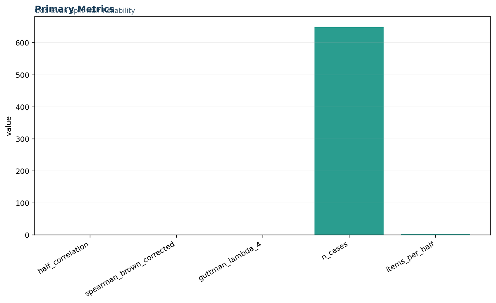
Primary Metrics
The primary-metrics chart places the half correlation, corrected reliability, Guttman lambda-4, case count, and items per half in one figure. Because 649 is on a completely different scale from coefficients near .24 to .38, the case-count bar dominates the axis and the reliability bars appear close to zero. The correct interpretation comes from the exact values: r=.236380, Spearman-Brown=.382375, lambda-4=.380733, n=649, and three items per half.
The scale difference is a visualization issue, not a calculation issue. Use the exact labels and result table when comparing coefficients.
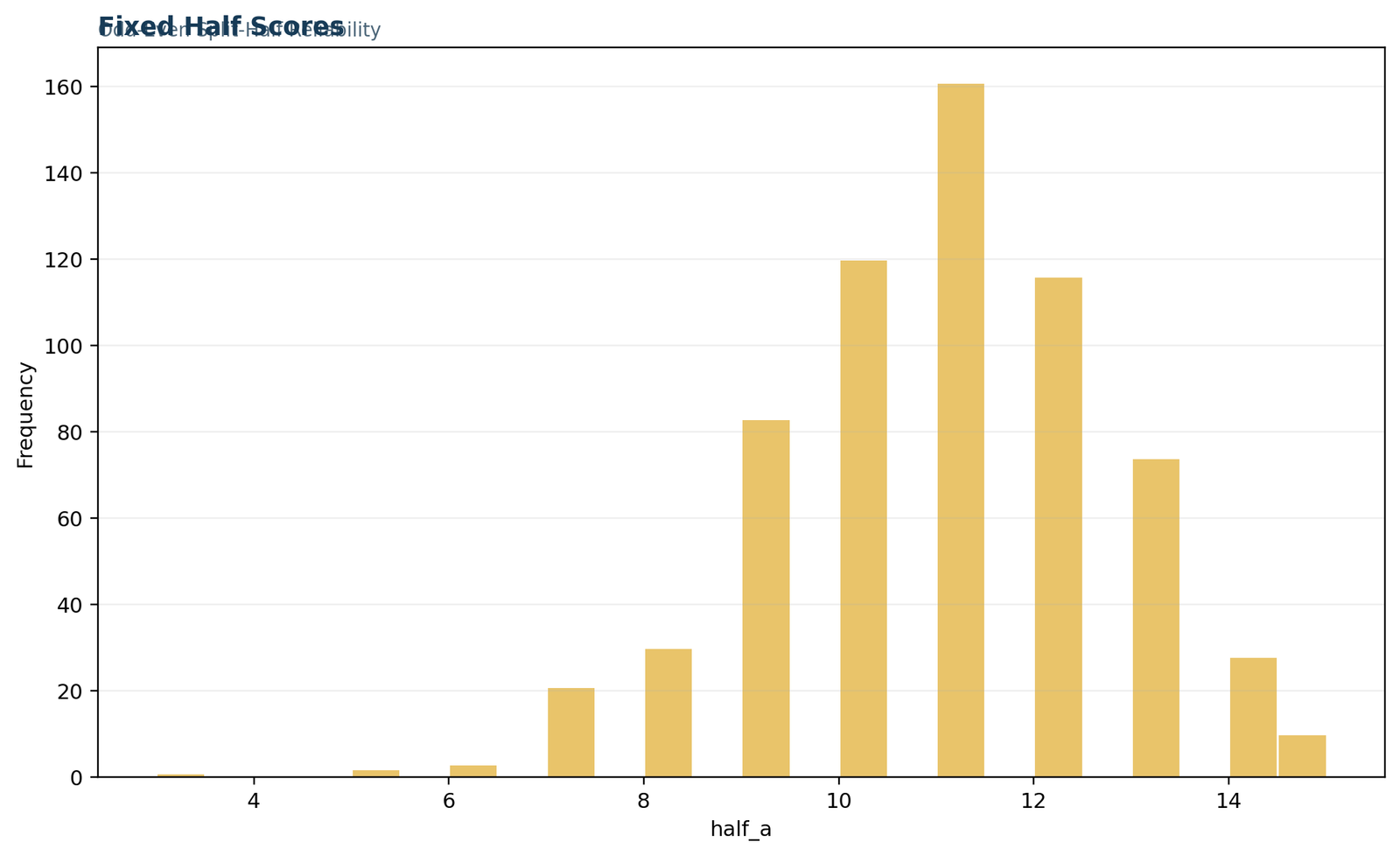
Fixed Half Scores
The frequency chart displays the distribution of Half A totals from 3 to 15. Most respondents scored near the upper-middle part of the possible range, with the highest frequency around 11. The distribution shows enough variation to calculate a correlation, but it is concentrated rather than uniform. Half A had a mean of 10.8351 and a variance of 3.20271.
The chart also confirms that the row-sum transformation produced valid integer totals within the expected range.
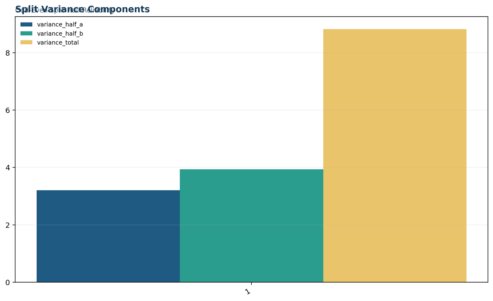
Split Variance Components
This chart compares the sample variance of Half A, Half B, and the total score. Half B was slightly more variable than Half A: 3.93708 versus 3.20271. The total variance was 8.81855. These three quantities enter the Guttman lambda-4 formula directly and yield .380733.
The total variance exceeds the sum of the half variances because the half scores have positive covariance, but the additional shared component is small.
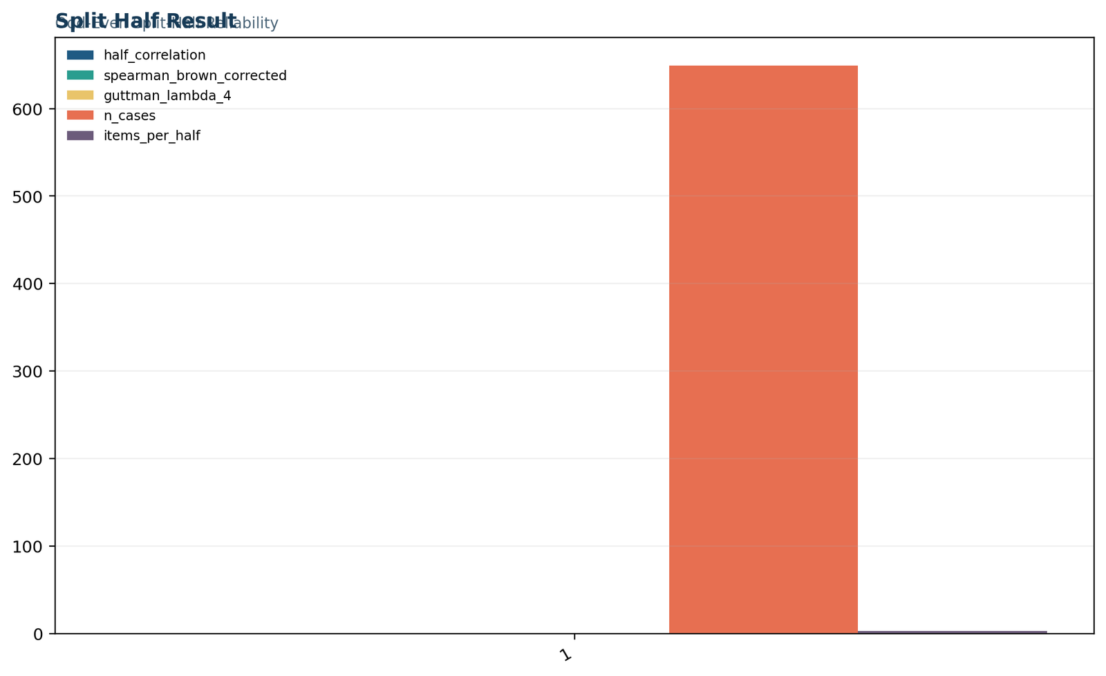
Split Half Result
The result chart combines the five final metrics. Again, n=649 compresses the coefficient bars. Read the chart as a verification dashboard rather than as a visual comparison of magnitudes. The two reliability estimates are nearly identical, while the raw half correlation is lower because it describes two shorter forms.
The equal item count of three per half confirms that the standard equal-length Spearman-Brown correction is appropriate.
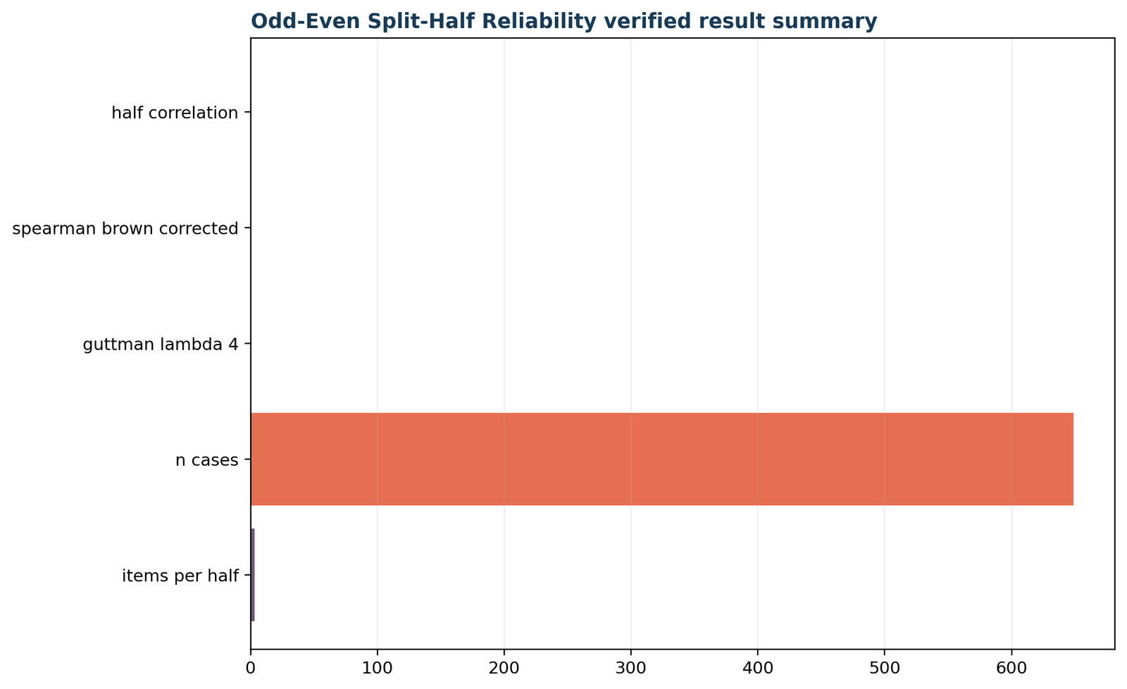
Verified Result Summary
The horizontal summary provides a final visual record of the verified metrics. The long n-cases bar confirms the sample size, and the short items-per-half bar confirms the balanced design. The reliability bars are difficult to see because they are measured on the same axis, so the exact report values remain essential.
The key conclusion is not that the bars are small relative to 649; it is that both reliability coefficients are approximately .38 on their natural 0-to-1 interpretation scale.
Read the five figures as one verification sequence: the first presents the headline metrics, the middle figures show the score distribution and variance structure, and the final figures document the corrected coefficients and cross-software agreement. Exact labels should be used whenever the common plotting scale compresses coefficients beside the sample size.
The verified Python split half reliability workflow was designed as a standalone analysis rather than a transcription of SPSS output. It read the source rows, constructed reverse-scored variables, declared the fixed halves, calculated row totals, and generated the final metric ledger and five charts. Independent calculation is important because agreement among separate implementations provides stronger evidence than repeatedly displaying one software’s rounded result.
Recommended Python Workflow
- Validate that each source item contains the expected 1-to-5 values.
- Create Dalc_R and Walc_R with the declared reverse transformation.
- Create Half A from famrel, goout, and Walc_R.
- Create Half B from freetime, Dalc_R, and health.
- Apply one documented missing-data rule to both half scores.
- Calculate the half correlation, Spearman-Brown correction, and lambda-4.
- Export exact values, not only rounded chart labels.
- Compare the metric ledger with R, SPSS, and Excel.
The Python report returned the exact values shown throughout this guide. Because the same 649 cases were used for every metric, differences are limited to floating-point rounding. The method is reproducible and suitable for automated batches when each instrument has its own declared item allocation and scoring rules.
Split Half Reliability in R: Complete Calculation and Charts
R independently reproduces the same five figures, formulas, and numerical results.
The R split half reliability implementation used the same transformations, fixed item allocation, complete-case scope, sample-variance convention, and formulas. It reproduced the Python and Excel results to floating-point precision. The duplicated visual structure is intentional: it makes cross-software checking direct and prevents differences in plotting style from being mistaken for differences in statistical results.
R Primary Metrics
The R primary metrics are r=.2363801915, Spearman-Brown=.3823746015, Guttman lambda-4=.3807326635, n=649, and three items per half. Agreement at this precision shows that the result is not tied to a particular software package. The chart’s common axis makes the case count visually dominant, so report the coefficient values in text.
Independent replication is strongest when data transformations, missing-data rules, and variance definitions are also identical.
R Fixed Half Scores
The distribution confirms the exact same Half A totals used in Python and Excel. Scores cluster around 10 to 12, with fewer cases at the minimum and maximum. This shape is consistent with a sum of three bounded items. The limited score range is one reason a three-item half may not discriminate respondents strongly enough to produce a high correlation.
A longer, more coherent item set would generally provide more score levels and more stable covariance information.
R Variance Check
R reproduced variance Half A=3.20271, variance Half B=3.93708, and total variance=8.81855. The values demonstrate why lambda-4 is around .381. The numerator of the error component remains large relative to total variance, leaving a limited proportion attributable to consistency between halves.
This independent variance check is valuable because it verifies the result without relying only on the correlation correction.
R Final Result
The final R chart packages the same five outputs used in the report ledger. The Spearman-Brown and Guttman values are nearly indistinguishable numerically, reinforcing the conclusion of low reliability. The large case count makes the estimate precise, but precision does not turn a small coefficient into a strong one.
Researchers should distinguish sample-size evidence from coefficient magnitude when interpreting statistically significant correlations.
R Verified Summary
The R summary closes the verification chain. Python, R, SPSS, and Excel all support the same practical decision: the six-item composite has weak split half reliability in this sample. The chart should be read alongside the part alpha warnings and the variable definitions, because those diagnostics explain why the coefficient is low.
Cross-software agreement confirms correctness of computation, not adequacy of the instrument.
Read the five figures as one verification sequence: the first presents the headline metrics, the middle figures show the score distribution and variance structure, and the final figures document the corrected coefficients and cross-software agreement. Exact labels should be used whenever the common plotting scale compresses coefficients beside the sample size.
R reproduced the fixed-score analysis with the same item transformations and formulas. The calculated half correlation was 0.236380191523515, the corrected coefficient was 0.38237460150868, and lambda-4 was 0.380732663549638. The last digits differ from Python only because floating-point numbers are printed with different precision.
Recommended R Workflow
- Keep the item allocation in an explicit object or documented list.
- Use row-wise sums only after verifying reverse scoring and missingness.
- Use the same complete-case subset for correlation and variance calculations.
- Use sample variances consistently for the lambda-4 calculation.
- Export a text or PDF result ledger with the full numeric precision.
- Generate charts from the same verified results object used in reporting.
R is particularly useful when researchers want to evaluate multiple theoretically justified splits, bootstrap the coefficient, or integrate reliability checks into a larger psychometric workflow. Any repeated-split extension should still distinguish exploratory optimization from a prespecified primary split.
Split Half Reliability in SPSS: Fixed Split and Output Interpretation
The SPSS RELIABILITY procedure reports both half alphas, the correlation between forms, Spearman-Brown, and Guttman output.
SPSS provides a dedicated split half reliability model within Reliability Analysis. The most important preparation is the order of variables. SPSS defines Part 1 from the first specified items and Part 2 from the remaining items according to the split point. For a fixed three-and-three design, place the three Half A items first and the three Half B items second.
Prepare scoring
Create Dalc_R=6-Dalc and Walc_R=6-Walc, verify ranges, and preserve the original variables for auditing.
Open Reliability Analysis
Choose Analyze, Scale, Reliability Analysis. Move famrel, goout, Walc_R, freetime, Dalc_R, and health into the Items box in that exact order.
Select the split-half model
Choose Split-Half and set the first part to three items. Request descriptives for items and scales, correlations, item-total statistics, means, and variances.
Read Reliability Statistics
SPSS reports Part 1 alpha, Part 2 alpha, total item count, correlation between forms, equal- and unequal-length Spearman-Brown coefficients, and the Guttman split-half coefficient.
Verify the actual half totals
Compute half_A and half_B explicitly, request their correlation and descriptives, and compare them with the Reliability Statistics table. The explicit correlation was .236 with 649 cases.
How to Interpret the SPSS Output Tables
Case Processing Summary: all 649 cases were valid and none were excluded. This eliminates changing sample size as an explanation for differences among software results.
Reliability Statistics: Part 1 alpha was -.348 and Part 2 alpha was -.044. SPSS correctly warned that the negative values result from negative average covariance among items. The correlation between forms was .236. Both Spearman-Brown coefficients were .382 because the halves were equal in length. Guttman split-half was .381.
Item Statistics: item means ranged from 3.1803 for freetime to 4.4977 for Dalc_R. Standard deviations ranged from .92483 for Dalc_R to 1.44626 for health. These descriptive differences show that the items do not have identical distributions.
Inter-Item Correlation Matrix: correlations ranged from -.389 between goout and Walc_R to .617 between Walc_R and Dalc_R. The mixture of positive and negative relationships is consistent with a broad behavioral item set rather than a single homogeneous scale.
Item-Total Statistics: corrected item-total correlations ranged from -.105 to .227, with several values negative or close to zero. These results support the low split half reliability conclusion and indicate that no simple interpretation of a unified composite is justified.
Scale Statistics: Half A mean=10.8351 and variance=3.203; Half B mean=11.2142 and variance=3.937; total mean=22.0493 and variance=8.819. These rounded SPSS values match the exact variance ledger.
Split Half Reliability in Excel: Worked Formula Calculation
The workbook exposes the half scores, variance components, correlation, substituted formulas, and final estimates.
The worked Excel split half reliability analysis is formula-driven and organized into six sheets: Guide, Data_Input, Working, Calculations, Diagnostics, and Reporting. Source data remain separate from transformations and results, which makes the workbook easier to audit.
Data input
Store the six original variables in clearly labeled columns and keep one row per respondent.
Working columns
Calculate Dalc_R and Walc_R, then calculate Half A, Half B, and Total for all 649 rows.
Correlation formula
Use Excel’s correlation function on the complete Half A and Half B ranges. The workbook returned 0.2363801915235146.
Spearman-Brown formula
Use two times the correlation divided by one plus the correlation. The workbook returned 0.38237460150867986.
Guttman lambda-4
Use sample variances for Half A, Half B, and Total in the variance formula. The workbook returned 0.3807326635496364.
Verification sheet
Compare workbook formulas with independently supplied reference values and calculate absolute differences. Every reported difference was at or below floating-point precision.
The Excel workbook is useful for teaching because every transformation and formula can be inspected. It is also suitable as an audit companion to SPSS, Python, or R, but the final interpretation should not rely on cell color or a single dashboard. The construct and item diagnostics remain central.
Spearman-Brown Correction, Guttman Lambda-4 and Split Choices
Understand what the correction changes, what it cannot repair, and why the chosen split matters.
Split half reliability coefficients are commonly read on a 0-to-1 scale, with larger values indicating greater consistency. Negative values are possible but usually signal a scoring or construct problem. There is no universal threshold because acceptable precision depends on purpose. A classroom research scale used to compare groups may tolerate more error than a clinical or licensing decision about one person.
| Approximate coefficient | General description | Practical interpretation |
|---|---|---|
| Below .50 | Very low | Substantial inconsistency; review scoring, dimensionality, and item content |
| .50 to .69 | Low to questionable | May be inadequate for many decisions; interpretation requires strong context |
| .70 to .79 | Often acceptable for early group research | May support low-stakes comparisons, subject to other evidence |
| .80 to .89 | Good | Stronger consistency for many research uses |
| .90 and above | Very high | Useful for high precision, although extreme redundancy should be checked |
These categories are heuristics, not fixed legal rules. The .382375 coefficient in the worked example falls clearly in the very-low range. The conclusion is strengthened by negative part alphas and weak corrected item-total correlations. The composite should not be used as though it were a precise single-scale measure.
Statistical Significance Versus Reliability Magnitude
The half correlation was statistically significant because n=649 provides high power to detect a small association. Reliability interpretation depends primarily on magnitude and measurement purpose, not whether p is below .05. A statistically significant r=.236 still represents weak agreement between the two shorter forms.
What the Result Suggests for This Item Set
The six variables may be better treated as separate indicators or grouped into theoretically coherent subdomains rather than forced into one total. A revised instrument could include multiple items for family support, social behavior, health, and substance-use behavior, then evaluate each subscale separately. Any revised structure should be tested in an independent sample and supported by construct-validity evidence.
Split Half Reliability Compared With Other Reliability Methods
Choose the coefficient that matches the measurement design and the intended source of consistency.
| Method | Main question | Data requirement | Key distinction |
|---|---|---|---|
| Split half reliability | Do two parts of one instrument produce consistent scores? | One administration and a declared split | Result depends on the selected division |
| Cronbach’s alpha | How consistently do items covary under the alpha model? | One administration | Averages information across item partitions |
| McDonald’s omega | How reliably does a factor-based composite measure a construct? | One administration and a defensible factor model | Uses model-based loadings rather than equal-item assumptions |
| Test-retest reliability | Are scores stable across time? | Two administrations | Includes temporal change and memory effects |
| Parallel-forms reliability | Do two independently built equivalent forms agree? | Two forms | Requires evidence that forms are parallel |
| Intraclass correlation | How much score variance reflects targets rather than error? | Repeated ratings or measurements | Multiple ICC models answer different agreement questions |
| Cohen’s kappa | Do two raters agree on categories beyond chance? | Categorical ratings | Not an internal-consistency coefficient |
No single split half reliability statistic is sufficient for every instrument. A comprehensive evaluation may combine internal consistency, temporal stability, rater agreement, measurement invariance, and validity evidence. Use the statistic that matches the score interpretation and source of error.
Related Statistical Guides
Diagnostics, Sensitivity Checks and Common Mistakes
Use the result as a measurement diagnostic, not merely as a number to classify.
A trustworthy split half reliability analysis does not end with the corrected coefficient. Researchers should inspect the internal behavior of each half, the relationship between the two halves, score ranges, coding direction, variance balance, item content, missing-data scope, and sensitivity to alternative defensible splits.
Check item coding
Negative part alphas and negative inter-item correlations can indicate reversed direction, heterogeneous content, or both. Reversing Dalc and Walc aligns direction but does not guarantee that all six variables measure one construct.
Check half balance
The halves should be comparable in item count, content coverage, score range, and variance. Equal length alone is insufficient when one half captures a different domain.
Check split sensitivity
A single split can be unusually favorable or unfavorable. Compare several defensible splits or use coefficients such as Cronbach’s alpha or McDonald’s omega when a broader item-level estimate is needed.
Check score distributions
Floor effects, ceiling effects, limited ranges, and sparse totals can weaken the correlation between half scores even with a large sample.
Check missing data
The reported analysis used 649 complete cases and excluded none within the selected six variables. Different missing-data rules can change the covariance structure and the coefficient.
Check substantive coherence
Reliability is not created by software. Items must have a defensible common construct before their internal consistency is summarized.
| Common mistake | Why it is wrong | Better practice |
|---|---|---|
| Reporting only the corrected coefficient | Readers cannot evaluate the raw agreement between halves. | Report the half correlation and the Spearman-Brown result together. |
| Choosing the split after seeing results | The reported coefficient becomes selectively optimized. | Predeclare the split or report a principled sensitivity analysis. |
| Treating a large sample as high reliability | Sample size affects precision, not coefficient magnitude. | Interpret the coefficient itself and its practical consequences. |
| Ignoring negative item relationships | Negative covariance can reveal coding or construct problems. | Inspect the inter-item matrix and item-total diagnostics. |
| Calling reliability validity | A consistent score can still measure the wrong construct. | Evaluate reliability and validity as separate evidence. |
How to Report Split Half Reliability in APA Style
Report the split rule, items, sample, raw correlation, correction, and substantive conclusion.
Complete Reporting Checklist
- Name the instrument or composite and explain why internal consistency is relevant.
- State the exact split rule and list the items in each half.
- Report the number of valid cases and how missing data were handled.
- Report the correlation between half scores.
- Name and report the correction formula.
- Report Guttman lambda-4 when used as a cross-check.
- Describe the magnitude in relation to the intended score use.
- Disclose major warnings such as negative part alpha values.
APA-Style Example for the Verified Analysis
A fixed balanced split-half analysis was conducted for six transformed items among 649 complete cases. Half A included famrel, goout, and Walc_R, whereas Half B included freetime, Dalc_R, and health. The half scores were positively correlated, r=.236, p<.001. The Spearman-Brown corrected split half reliability coefficient was .382, and Guttman lambda-4 was .381. Part-specific alpha estimates were negative (Part 1 α=-.348; Part 2 α=-.044), indicating weak and inconsistent covariance within the two halves. The six-item composite therefore demonstrated low internal consistency in this sample.
Short Results Sentence
The fixed three-item halves showed low consistency, r=.236, Spearman-Brown=.382, and Guttman λ4=.381, n=649.
How Not to Report the Result
Do not state only that the correlation was significant. Do not label .382 as acceptable because the p-value is small. Do not omit the split rule or negative part alphas. Do not imply that software agreement proves construct validity. Good reporting connects the coefficient to score use and explains the limitations revealed by diagnostics.
Split Half Reliability PDF, Excel and Software Downloads
Four files provide the complete cross-software audit trail.
Download the four reproducible files used for this split half reliability worked example. The Python, R, and SPSS PDF reports document the independent software outputs, while the Excel workbook exposes the calculations and substituted formulas.
R reportIndependent R replication of the same fixed split.Open R PDF →
SPSS outputReliability Statistics, descriptives, correlations, and graph.Open SPSS PDF →
Worked Excel analysisHalf scores, formulas, variance checks, and final estimates.Download workbook →
Verification Sources and Cross-Software Agreement
A transparent audit of the exact values, transformations, and rounding.
The numerical claims in this split half reliability guide are supported by the software reports and worked workbook rather than by an unsupported demonstration. The same fixed split, case scope, scoring rules, and sample-variance convention were used in every implementation.
SPSS verification
The SPSS Reliability Statistics table reports a correlation between forms of .236, equal-length and unequal-length Spearman-Brown coefficients of .382, and a Guttman split-half coefficient of .381. The Case Processing Summary reports 649 valid cases and no excluded cases for the six selected variables.
The SPSS descriptive output gives Half A mean = 10.8351, variance = 3.203, and SD = 1.78961; Half B mean = 11.2142, variance = 3.937, and SD = 1.98421.
Independent replication
Python, R, and Excel preserve more decimal places and reproduce the same values: half correlation = 0.2363801915, Spearman-Brown = 0.3823746015, and Guttman lambda-4 = 0.3807326635.
Agreement at this precision demonstrates that the result does not depend on one software package. It does not remove the need to interpret the negative part alphas and weak item coherence.
| Verification item | Expected value | Where to check |
|---|---|---|
| Valid cases | 649 | SPSS Case Processing Summary and all reports |
| Half A items | famrel, goout, Walc_R | Data dictionary and software syntax |
| Half B items | freetime, Dalc_R, health | Data dictionary and software syntax |
| Correlation between forms | 0.236380 | SPSS Reliability Statistics and Python/R reports |
| Spearman-Brown coefficient | 0.382375 | All four implementations |
| Guttman lambda-4 | 0.380733 | SPSS output and variance-based workbook check |
Split Half Reliability FAQs
Twelve direct answers to the most common methodological and reporting questions.
These split half reliability FAQs answer the most common questions about meaning, formulas, acceptable values, split selection, software, interpretation, and reporting.
What is split half reliability?
Split half reliability is an internal-consistency method that divides one test or scale into two predeclared, comparable halves, calculates a score for each half, correlates those scores, and then applies a length correction. The uncorrected correlation describes agreement between the two shorter forms. The Spearman-Brown coefficient estimates the reliability expected for the original full-length instrument. In this worked example, the two three-item half scores correlated at 0.236380, and the Spearman-Brown corrected estimate was 0.382375. That result is low for most decisions requiring dependable individual scores, so the six items should not be treated as a strongly homogeneous scale without further construct review.
What does split half reliability measure?
Split half reliability measures the degree to which two parts of one instrument rank or differentiate respondents in a similar way. It does not directly measure stability across time, agreement between raters, or validity. The first statistic is the correlation between half scores. Because each half contains fewer items than the complete instrument, the half correlation is normally adjusted with the Spearman-Brown formula. The resulting coefficient is interpreted as an estimate of full-length internal consistency for that specific split. Guttman lambda-4 provides a closely related variance-based estimate and is useful as a cross-check.
How do you calculate split half reliability?
First, define two balanced halves before looking at the final coefficient. Second, calculate one total score for each half for every complete case. Third, compute the Pearson correlation between the two half scores. Fourth, correct the correlation for test length with 2r divided by 1 plus r. In the verified example, r was 0.236380, so the corrected value was 2(0.236380)/(1.236380)=0.382375. A variance-based check gave Guttman lambda-4=0.380733. Report the split rule, number of items per half, sample size, half correlation, corrected coefficient, and any evidence that the halves were not internally coherent.
What is the Spearman-Brown formula for split half reliability?
For two equal-length halves, the Spearman-Brown formula is rho = 2r/(1+r), where r is the observed correlation between the two half scores. The formula corrects for the fact that the correlation was calculated from forms that are only half as long as the original test. When r=0.236380, the corrected estimate is 0.382375. The correction improves the estimate mathematically, but it cannot repair mismatched content or negatively related items. Therefore, the Spearman-Brown result should be interpreted together with the split design, item correlations, half variances, and substantive meaning of the items.
What is Guttman split half reliability?
Guttman split half reliability usually refers to Guttman lambda-4, a variance-based coefficient for a selected two-part split. It uses the variances of the two half scores and the variance of the total score. The formula used in this example is 2[1-(variance A + variance B)/variance total]. With half variances of 3.20271 and 3.93708 and total variance of 8.81855, lambda-4 was 0.380733. It was almost identical to the Spearman-Brown estimate of 0.382375, which confirms that the low reliability conclusion is not an artifact of rounding or software.
What is a good split half reliability score?
There is no universal cutoff for every instrument. Values around 0.70 are often treated as a minimum for early group-level research, while higher-stakes decisions generally require stronger evidence, often 0.80 or 0.90 depending on consequences. These are conventions, not laws. A coefficient must be interpreted in relation to test purpose, score use, construct breadth, number of items, sample, and measurement error. The verified coefficient of 0.382375 is well below common expectations and indicates that these six transformed items do not function as a dependable single scale in this sample.
How do you interpret a low split half reliability coefficient?
A low split half reliability coefficient means that people who score relatively high on one half do not consistently score high on the other half. Possible reasons include multidimensional content, a poor split, too few items, restricted variance, reverse-scoring errors, weak item-total relationships, or items that intentionally measure different behaviors. In the worked analysis, each half contained only three items, both within-half alphas were negative, and several correlations were negative. These diagnostics suggest a substantive lack of homogeneity rather than a minor rounding problem. The correct response is to review the construct and item coding, not merely to report the corrected coefficient.
How is split half reliability different from Cronbach’s alpha?
Split half reliability evaluates one chosen division of the items, whereas Cronbach’s alpha summarizes the average behavior across many possible item partitions under its model. A particular split can look better or worse depending on how items are allocated. Alpha is less dependent on one split but still relies on assumptions and can be misleading for multidimensional scales. Use the split half result to understand a transparent, theory-based division, and compare it with a broader internal-consistency analysis. The Cronbach’s alpha guide and corrected item-total correlation guide provide complementary diagnostics.
How is split half reliability different from test-retest reliability?
Split half reliability uses one administration and compares two item sets, so it addresses internal consistency at one point in time. Test-retest reliability administers the same instrument on two occasions and evaluates temporal stability. A scale can have high internal consistency but low stability if the construct changes, and it can have stable total scores while containing heterogeneous items. The method should match the source of consistency that matters. For a one-time educational or psychological scale, split half reliability may be useful; for a stable trait measured across weeks, test-retest evidence is usually also needed.
When should split half reliability be used?
Use split half reliability when an instrument is intended to measure one reasonably coherent construct, all items are administered once, a meaningful balanced split can be declared, and the researcher wants a transparent internal-consistency check. It is particularly useful for achievement tests with many items spanning comparable content or for a scale where odd-even allocation balances item order effects. Avoid relying on it alone when the instrument is multidimensional, has very few items, contains speeded sections, uses branching logic, or has halves that differ substantially in content or difficulty.
Does split half reliability require a random split?
No. A random split is one option, but it is not automatically the best option. A fixed odd-even or content-balanced split is often easier to reproduce and may better preserve comparable item content and difficulty. Random splitting can produce unstable coefficients, especially with a small number of items. The key requirement is to declare the rule before examining the result and explain why the halves are comparable. This worked analysis used a fixed balanced split with three items in each half so Python, R, SPSS, and Excel could reproduce exactly the same coefficient.
What are the advantages of split half reliability?
The method requires only one administration, reduces burden compared with test-retest or alternate-form designs, produces a clear correlation that readers can understand, and can be reproduced easily when the split is fixed. It also supports a direct Spearman-Brown calculation and a Guttman lambda-4 check. Because the two scores are created from the same respondents at the same time, temporary changes between sessions do not contaminate the estimate. Split half reliability is therefore efficient for an initial evaluation of internal consistency, provided the instrument has enough items and the two halves are defensibly balanced.
Related Statistical Guides
Continue with reliability, correlation, measurement, and diagnostic methods.