
Test Retest Reliability: 7 Essential Steps, Formula and Worked Example
Test retest reliability evaluates whether the same measurement produces stable scores when it is administered to the same people on two occasions. This worked guide separates rank-order stability, systematic change, and within-person measurement error so a high correlation is not mistaken for perfect agreement.
What did the test retest reliability analysis show?
The first and second scores were strongly associated, r = 0.864982, with n = 649 matched observations and p < .001. The retest score was slightly higher on average: the mean change defined as G2 − G1 was 0.1710, 95% CI [0.0570, 0.2851], t(648) = 2.945, p = .003. The change-score standard deviation was 1.4793, and the within-person standard error of measurement estimated as SD(change)/√2 was 1.0460.
The practical conclusion is strong rank-order stability with a small but statistically detectable upward shift. Test retest reliability is therefore good in the correlational sense, but the measurements are not perfectly interchangeable because the second administration shows systematic drift and individual differences around that drift.
Quick result ledger
What is test retest reliability?
A direct definition of temporal stability and the limits of a correlation-only interpretation.
Test retest reliability is the consistency of scores obtained when the same instrument is administered to the same participants on two different occasions. Test retest reliability asks whether people who score relatively high at the first administration also tend to score relatively high at the second, and whether people who score relatively low remain comparatively low. In psychology, education, health research, survey design, and performance testing, this is often described as temporal stability or stability reliability.
The core question
Imagine a questionnaire intended to measure a stable trait. The same group completes it today and again after an appropriate interval. A reliable instrument should preserve the ordering of respondents unless the construct genuinely changes. When the first and second scores follow the same pattern, the test retest reliability coefficient is high. When the ordering changes substantially, the coefficient is low.
The coefficient is commonly calculated with Pearson correlation for continuous scores, although an intraclass correlation coefficient may be preferable when absolute agreement is the main goal. For ordinal categories, weighted kappa or rank correlation may be more defensible.
Why the word reliability matters
Reliability concerns consistency, not truth. A measure can produce nearly identical scores at both occasions and still fail to measure the intended construct. That is why test retest reliability does not by itself establish validity. It only shows whether the observed scores are reproducible across time under the specified conditions.
This distinction also separates test retest reliability from Cronbach’s alpha. Alpha evaluates the internal consistency of multiple items measured at one occasion. Test retest reliability evaluates stability of total scores or measurements across occasions. A scale can have high alpha but weak temporal stability, or moderate alpha but strong stability, because the two methods answer different questions.
In an AP Psychology definition, test retest reliability is often summarized as giving the same test to the same group twice and correlating the two sets of scores. That summary is useful, but a complete statistical analysis also checks whether the average score changed and whether the magnitude of within-person differences is small enough for the intended use. A large positive correlation can exist even when every participant gains several points, so correlation alone does not guarantee interchangeability.
When should test retest reliability be used?
Use it when the same construct, instrument, scoring rule, and units are measured twice under comparable conditions.
Test retest reliability is appropriate when researchers need evidence that observed scores are stable over time. Test retest reliability is most informative when the target characteristic is not expected to change materially between administrations. Examples include established personality tendencies, aptitude scores, stable knowledge under no-intervention conditions, equipment measurements, and ratings of persistent characteristics.
Suitable designs
The same respondents, objects, or units are measured twice with the same scoring rule. The administration conditions should be comparable, the response scale should have adequate range, and the time interval should be specified before analysis. The design is naturally paired because every first score must correspond to the same unit’s second score.
Questionable designs
The method is difficult to interpret when an intervention occurs between occasions, when the attribute is expected to develop rapidly, or when seasonal, fatigue, learning, medication, or environmental effects are likely. In those settings, observed change may be real rather than measurement error.
Alternative designs
Use inter-rater reliability when different observers score the same targets, intra-rater reliability when the same observer repeats ratings, internal consistency when multiple items form a scale, and parallel-forms reliability when equivalent versions of a test are compared.
Choosing the retest interval
There is no universally correct interval. A very short interval can inflate test retest reliability because participants remember answers, repeat a strategy, or remain in the same temporary state. A very long interval can reduce stability because the construct genuinely changes. The best interval is long enough to limit memory and immediate carryover but short enough that real development, treatment, and major contextual change are unlikely.
The interval must be interpreted in relation to the construct. A few days may be reasonable for a stable laboratory measure but inappropriate for a school achievement test if students continue learning. Several weeks may work for a personality inventory but be too long for symptoms that fluctuate daily. The interval, administration mode, setting, and any events between occasions belong in the method section because test retest reliability is a property of scores under particular conditions, not a permanent property of an instrument in every population.
Test retest reliability assumptions: conditions to check
The design is repeated-measures, but reliable interpretation still depends on stable targets, correct pairing, comparable administration, and appropriate diagnostics.
The assumptions of test retest reliability include correct pairing, a stable target construct, comparable administration conditions, appropriate measurement level, adequate score variability, and a relationship consistent with the chosen coefficient. Additional assumptions apply to the paired t test and any ICC model.
Stable construct
The true attribute should not change meaningfully during the interval. If students receive instruction, patients receive treatment, or respondents experience a major event, change cannot automatically be labeled measurement error. The study design must distinguish expected true change from instability.
Comparable administration
Instructions, timing, device, language, scoring, environment, and assistance should be consistent. A paper test followed by a mobile retest, or a supervised test followed by an unsupervised retest, introduces method variance that may lower test retest reliability.
Correct pairing and independence
Each G1 value must be paired with the same participant’s G2 value. Different participants should be independent unless clustering is modeled. Duplicate IDs, row shifts, and merges based on incomplete names are common sources of false results.
Appropriate scale
Pearson correlation is designed for quantitative variables with a meaningful linear relationship. For ranks or strongly ordinal categories, Spearman rank correlation or weighted kappa may be more appropriate.
Linearity and influential cases
The scatterplot should show a roughly linear association. Curvature, separate clusters, and extreme leverage points can make Pearson r misleading. Review scatterplots and correlation alongside numerical output.
Adequate variability
Restricted score range reduces correlation even when repeated scores are precise. A sample containing only very similar participants can produce a lower coefficient than a heterogeneous sample using the same instrument. Reliability therefore depends partly on the sampled population.
Change-score normality
The paired t test assumes the distribution of differences is approximately normal, not that G1 and G2 must each be normal. In the worked data, Shapiro-Wilk W = .866 and p < .001, and the Q-Q plot shows tail departures. The sample size is large, so the mean comparison is generally robust, but the extreme differences should still be described. The histogram, Q-Q plot, skewness, and kurtosis are more informative than a binary normality decision alone. See the guides to the Shapiro-Wilk test, Q-Q plot normality check, and skewness and kurtosis.
Attrition and missingness
Participants who return for the retest may differ from those who do not. A high coefficient among completers does not remove attrition bias. Report the original sample, the retest completion rate, reasons for missingness, and differences between completers and noncompleters when available. The worked analysis has 649 complete pairs, so the coefficient, paired change, and error calculations use the same n.
Test retest reliability hypotheses
Separate the hypothesis about rank-order stability from the hypothesis about systematic mean change.
Stability hypothesis
H1: ρG1,G2 ≠ 0
The two-sided Pearson test asks whether the population correlation between the test and retest scores differs from zero. Rejecting this null establishes evidence of association, but it does not prove that the coefficient is large enough for the intended decision.
Systematic-change hypothesis
H1: μG2−G1 ≠ 0
The paired comparison asks whether the population mean change equals zero. A significant result indicates systematic drift even when the correlation is high.
For reliability evaluation, a significance test of r = 0 is rarely the main substantive target because even a modest coefficient can become significant in a large sample. The size of r, its confidence interval, the required reliability standard, and the consequences of measurement error are more important. A coefficient of .50 may be highly significant with hundreds of observations but still be inadequate for individual-level decisions.
Likewise, a significant paired mean difference does not automatically make the instrument unusable. With 649 pairs, the analysis detects an average increase of only 0.171 points. Researchers should judge whether that shift is large relative to the score scale, clinical threshold, grading decision, or smallest meaningful difference. The paired result identifies drift; domain knowledge determines its importance.
Test retest reliability formulas and calculation
The worked analysis combines Pearson stability, paired change, change-score variability, and a within-person error estimate.
The basic test retest reliability formula for continuous scores is Pearson’s product-moment correlation between the first and second administrations. The worked analysis supplements this coefficient with the mean change, change-score standard deviation, confidence interval, and within-person standard error of measurement.
The numerator is the cross-product of centered test and retest scores. The denominator scales the covariance by the variability at both occasions, producing a coefficient from −1 to +1.
Change-score equations
Measurement-error equation
This estimate assumes the two occasions contribute similar independent error variance. It is often called typical error or within-subject standard error. It is distinct from the conventional reliability-based SEM = SD√(1 − r), which depends on the selected score SD and reliability coefficient.
Worked substitution for Pearson stability
Using all 649 matched G1 and G2 values, the covariance and standard deviations produce r = 0.8649816303. The coefficient is positive and close to 1, showing that the participant ordering is largely preserved. Squaring the coefficient gives r² ≈ 0.7482, meaning roughly 74.8% of the linear variance in one occasion is shared with the other. This squared value is descriptive and should not be presented as the percentage of scores that are identical.
Paired confidence interval
The interval is entirely above zero, indicating a small positive average shift from G1 to G2. The corresponding paired statistic is t(648) = 2.9454, p = .00334.
For a nonnormal difference distribution, the paired t test is often robust with a large sample, but the distribution and outliers should still be inspected. A sensitivity analysis can use a Wilcoxon signed-rank test when the median or rank-based change question is more appropriate.
Test retest reliability example: 649 matched scores
The complete worked example identifies the variables first and then reconciles every verified result.
Test retest reliability is demonstrated with G1 as the first score and G2 as the second score for the same 649 students. The example preserves matched rows, defines change as G2 − G1, and reports stability, drift, individual change, and measurement error as separate results.
| Variable | Role | Measurement level | Observed summary | Interpretation in this analysis |
|---|---|---|---|---|
| G1 | Test score / occasion 1 | Continuous numeric score | Mean = 11.3991; SD = 2.7453 | Baseline measurement used to establish the first rank order. |
| G2 | Retest score / occasion 2 | Continuous numeric score | Mean = 11.5701; SD = 2.9136 | Repeated measurement compared with the baseline score. |
| Change | Derived score, G2 − G1 | Continuous paired difference | Mean = 0.1710; SD = 1.4793; median = 0 | Positive values indicate an increase at retest; negative values indicate a decrease. |
| Subject ID | Pairing key | Identifier | 649 unique matched rows | Ensures that each test score is matched to the correct retest score. |
The source data contain no missing values for G1 or G2 in the 649 retained rows. If one occasion were missing, that participant could not contribute to the paired correlation or change analysis without an explicit missing-data strategy. Pairwise deletion can create different sample sizes across statistics, so the report should always display the number of complete pairs.
Recommended long-format structure
A wide file with one row per participant and separate G1 and G2 columns is convenient for correlation and paired testing. A long file with columns for participant, occasion, and score is often better for data visualization, mixed models, repeated-measures analysis, and extension to more than two occasions. Whichever format is used, duplicate identifiers and accidental row sorting can break the pairing and invalidate test retest reliability.
Verified worked calculation
Step 1: inspect the occasions
G1 has a mean of 11.3991 and a sample SD of 2.7453. G2 has a mean of 11.5701 and a sample SD of 2.9136. The retest distribution is therefore slightly higher and slightly more dispersed. Similar means and SDs support comparability, but they do not establish person-level stability, so the paired association must be examined.
The score range and scatter show substantial overlap between occasions. Most points follow an upward diagonal pattern, which is what a strong test retest reliability result should look like. A few observations have unusually large changes and contribute to the heavy tails in the change distribution.
Step 2: calculate stability
The Pearson coefficient is 0.8649816303. Its p-value is approximately 6.37 × 10−196, which should be reported as p < .001. The coefficient indicates that participants generally retained their relative ranking. In many research contexts this would be described as good or strong temporal stability, while high-stakes individual decisions may require a stricter benchmark.
The coefficient is not perfect. The unexplained component reflects measurement error, temporary states, true individual change, restricted score precision, and potentially nonlinear or subgroup-specific patterns.
Step 3: calculate paired change
The mean G2 − G1 difference is 0.171032. The median difference is 0, showing that at least half of participants changed by no more than zero in the middle of the ordered distribution. The SD of the differences is 1.479289, while observed changes range from −9 to 11. Most changes cluster between −2 and +2, but rare extremes widen the range and produce strong kurtosis.
The 95% confidence interval [0.0570, 0.2851] indicates that the average population change is likely positive but small. The paired t result is statistically significant because the mean change is estimated precisely.
Step 4: estimate measurement error
Dividing 1.479289 by √2 gives 1.046015. Under the equal-error assumption, repeated scores for an unchanged person typically vary around the person’s latent score by about one point. This estimate helps translate test retest reliability into the original score units.
A rough 95% repeatability range for the difference can also be considered as mean change ± 1.96 × SD(change), giving approximately −2.728 to 3.070. This range is descriptive and shows that individual retest differences can be much wider than the small average shift.
Test retest reliability results and interpretation
The coefficient is strong, but the paired analysis also identifies a small upward shift and nontrivial person-level differences.
A test retest reliability coefficient near +1 indicates strong preservation of relative score ordering, a value near 0 indicates little linear stability, and a negative value indicates that high scores at one occasion tend to correspond to low scores at the other. Negative coefficients usually signal severe instability, coding problems, reversed scoring, or a highly unusual process.
| Coefficient pattern | Practical description | What to check | Why context matters |
|---|---|---|---|
| Below .50 | Weak temporal stability | Scoring errors, unstable construct, poor administration control, restricted range | May be unacceptable for most individual decisions but informative for rapidly changing states. |
| .50 to .69 | Moderate stability | Confidence interval and measurement purpose | Can support exploratory group research but may be inadequate for classification. |
| .70 to .79 | Often described as acceptable | Consequences of error and number of repeated measurements | No universal cutoff applies across disciplines. |
| .80 to .89 | Good or strong stability | Systematic bias and individual error | The worked value .865 falls here under common heuristics. |
| .90 and above | Very high stability | Memory effects, duplicated scoring, restricted task variation | High-stakes individual use often demands stronger evidence than research screening. |
These ranges are descriptive conventions, not laws. A coefficient of .80 may be adequate for comparing group averages but inadequate for deciding whether one person qualifies for treatment, certification, or placement. The acceptable threshold depends on the cost of incorrect decisions, the score’s role, the number of items, the retest interval, and whether repeated measurements are averaged.
Interpreting r = 0.864982
The worked coefficient indicates strong positive stability. People who scored higher at G1 generally scored higher at G2. However, the average retest score increased by 0.171, and the typical error is approximately 1.046 points. Therefore, the result supports use for group-level stability and many research purposes, while any individual-level classification should account for score uncertainty around cutoffs.
The correlation p-value is not the main evidence of quality. With n = 649, even a much smaller correlation would be significant. The coefficient magnitude, uncertainty, scatterplot, change distribution, and practical error scale provide the substantive interpretation. This follows the general principle described in effect size and statistical power guides.
Why high test retest reliability can coexist with systematic change
A common misunderstanding is that high test retest reliability means the two sets of scores are equal. Correlation only requires that participants move together in a consistent pattern. If every score rises by the same amount, the correlation remains 1. If high scorers increase slightly more than low scorers, the coefficient may still be extremely high.
Constant shift example
Suppose five first scores are 10, 20, 30, 40, and 50. The retest scores are 15, 25, 35, 45, and 55. Pearson r equals 1 because the rank order and linear spacing are unchanged. Yet every person is five points higher, so absolute agreement is poor if identical scores were expected.
A paired test would detect the five-point shift, and a difference plot would show every point at +5. This is why test retest reliability should include a change analysis.
Random error example
Now suppose changes are −6, +4, +1, −5, and +6. The mean change may be near zero, but the individual differences are large. A nonsignificant paired mean does not prove agreement because positive and negative changes can cancel.
The change-score SD, typical error, and limits of agreement reveal this problem. Reliability analysis needs both central tendency and spread.
The worked result
The example combines a high coefficient of .865 with a small positive mean change of .171. The average drift is statistically detectable, but the magnitude is modest. The more important person-level quantity is the change SD of 1.479 and the typical error of 1.046. These indicate that individual repeated scores can differ by around one point due to within-person variation even when the group ranking is strong.
The distribution is also nonnormal and heavy-tailed. One participant changed by −9 and another by +11. These rare values do not erase the overall stability, but they warn against assuming that every individual’s retest score will be close. Outlier review should investigate data entry, unusual circumstances, floor or ceiling effects, and genuine changes without automatically deleting valid observations.
Test retest reliability in Python: complete analysis and charts
The first Python chart is displayed alone; the remaining charts are arranged in paired rows exactly as in the supplied master format.
The Python implementation calculates the same test retest reliability metrics as the workbook and SPSS analysis. The first chart is intentionally shown alone so the primary result remains readable; the remaining charts are arranged in paired rows for efficient desktop and mobile viewing.
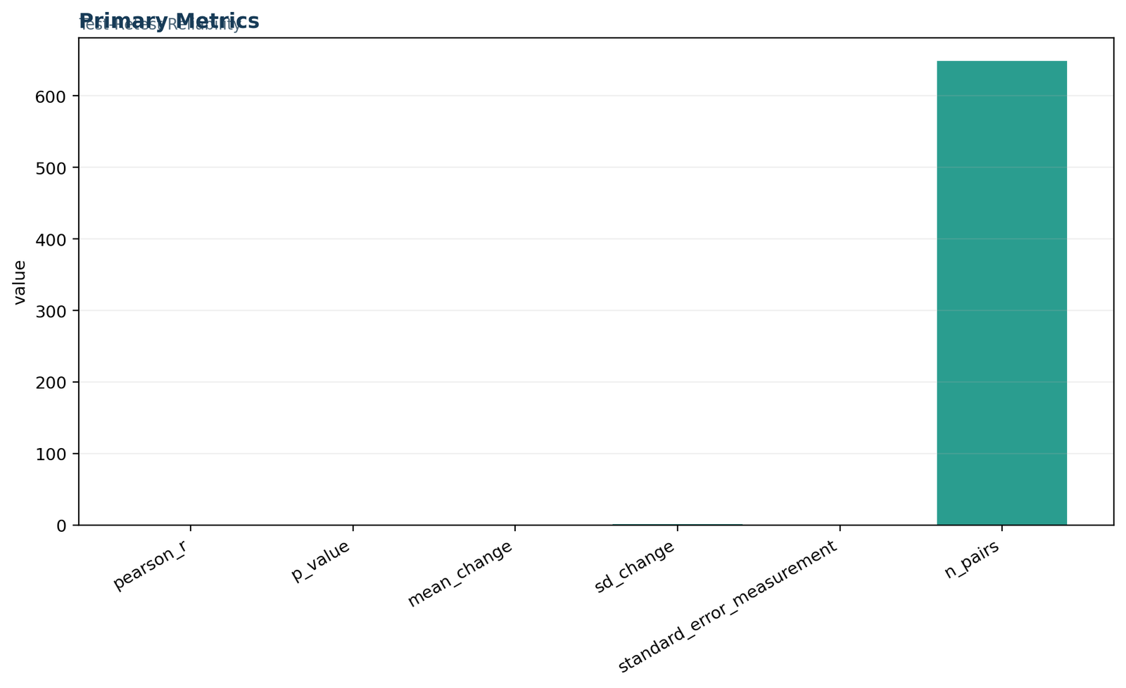
Python chart 1: Primary test retest reliability metrics
The headline chart consolidates r = 0.864982, n = 649, mean change = 0.1710, change SD = 1.4793, and SEM from change = 1.0460. The coefficient supports strong rank-order stability, while the change metrics prevent the result from being interpreted as exact agreement.
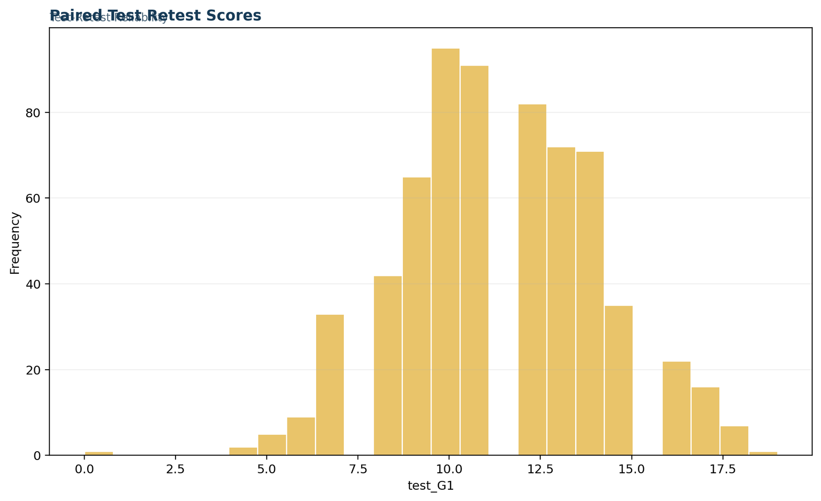
Python chart 2: Paired test and retest scores
The score pattern follows a clear positive diagonal. Higher G1 scores generally correspond to higher G2 scores, explaining the strong Pearson coefficient. Vertical spread at a fixed G1 value shows that participants with the same first score can still differ at retest.
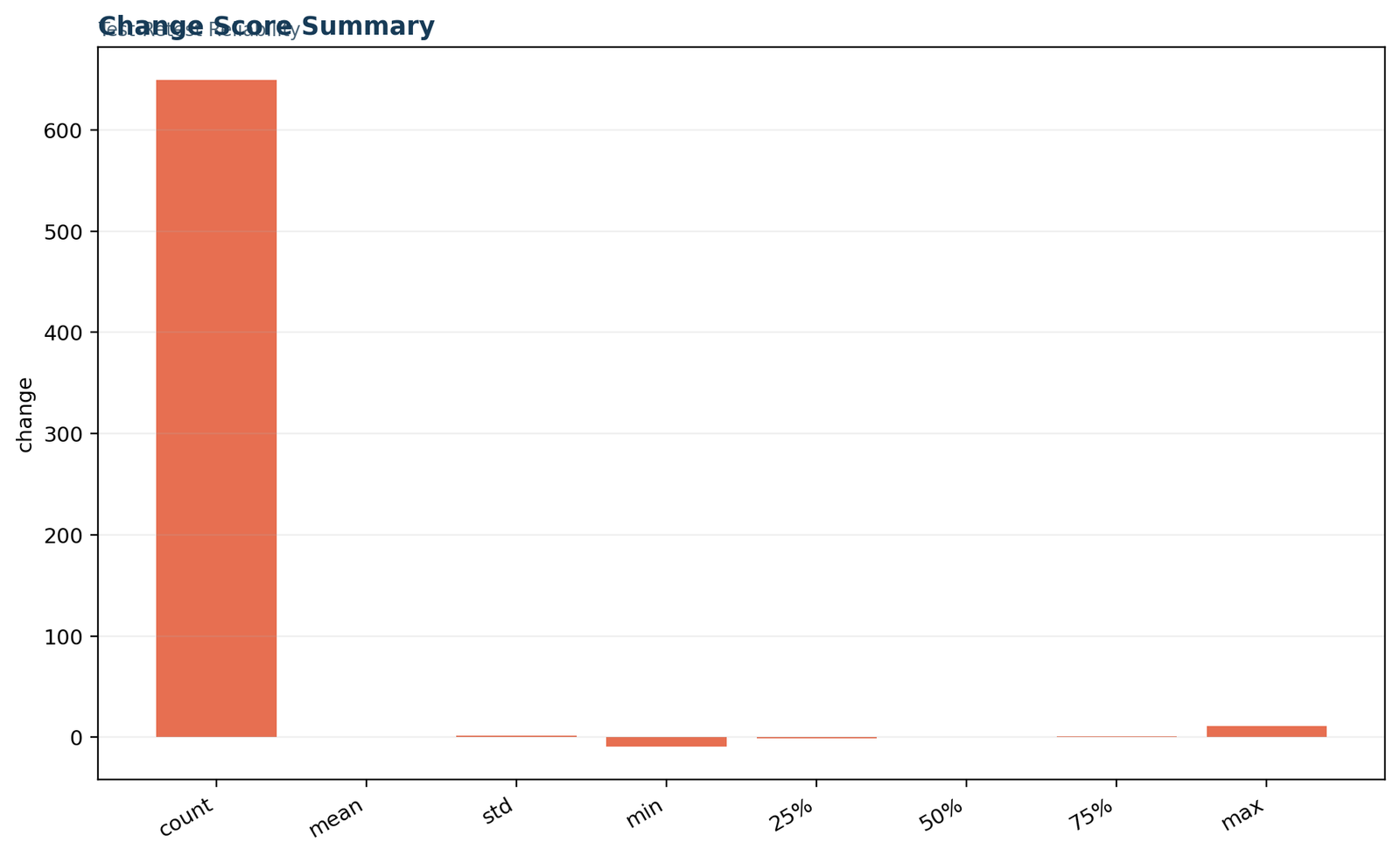
Python chart 3: Change-score summary
The difference distribution is centered near zero, with a mean of 0.171 and median of 0. Most observations show small changes, while a few large negative and positive differences create a range from −9 to 11 and heavy tails.
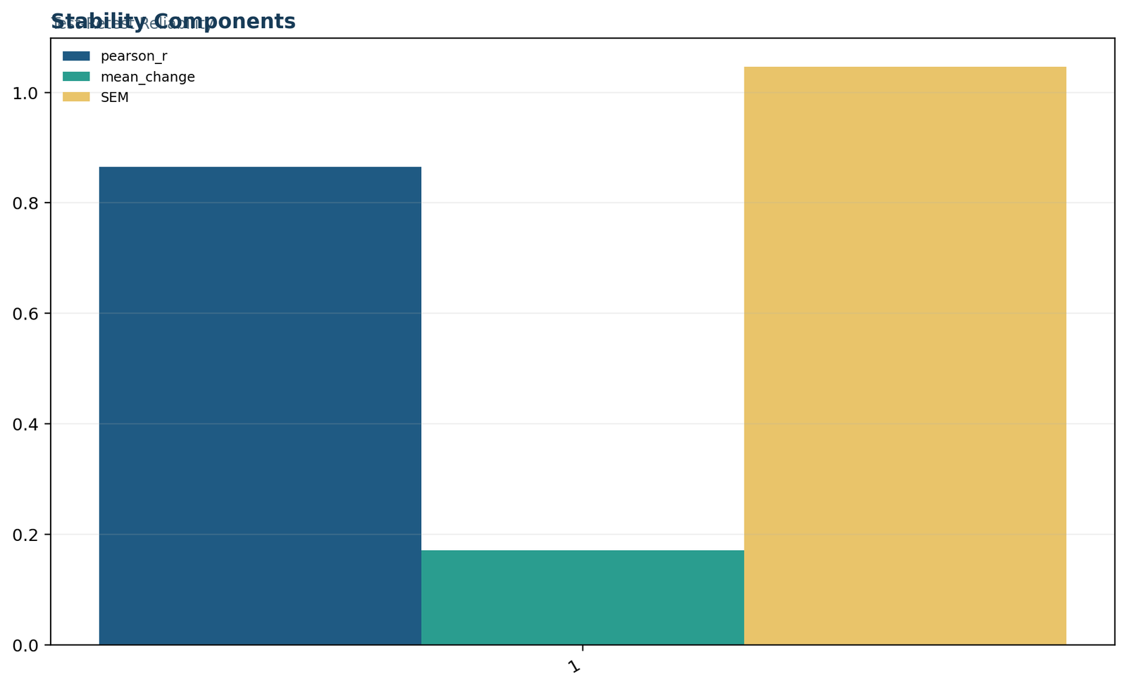
Python chart 4: Stability components
This chart separates the correlation coefficient from systematic drift and error in original score units. The separation is essential because the coefficient can remain high even when the retest mean shifts.
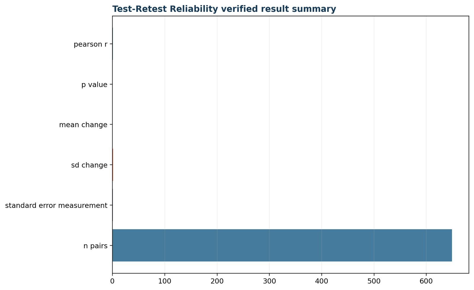
Python chart 5: Verified result summary
The verification panel confirms agreement among the independent calculations. Pearson r, mean change, change SD, measurement error, and matched sample size reconcile to numerical precision.
The Python charts answer different questions and should be read together. The first and second emphasize stability; the third emphasizes individual change; the fourth clarifies what each component represents; and the fifth documents reproducibility. No single image should replace the numerical result statement.
When adapting the Python workflow to another dataset, preserve participant pairing, convert relevant columns to numeric values, inspect missing cases before calculation, and use the same direction for the difference. Reversing G2 − G1 to G1 − G2 changes the sign of the mean difference but not the correlation or change-score SD.
Test retest reliability in R: independent verification and charts
The R workflow independently reproduces the coefficient, mean change, change-score SD, and measurement-error estimate.
The R analysis provides an independent cross-check of test retest reliability. Matching results across programming environments reduce the risk of a hidden formula, data orientation, missing-value, or denominator error. The same five verified images are organized with the first result alone and the remaining outputs in paired rows.
R chart 1: Primary reliability metrics
R returns r = 0.864982 and the same 649 complete pairs. The change calculation gives 0.1710 with SD 1.4793, and the equal-error estimate gives SEM = 1.0460.
R chart 2: Paired score relationship
The positive point pattern visualizes strong temporal ordering. The chart should be inspected for curvature, clusters, floor effects, ceiling effects, and influential observations before relying on a single Pearson coefficient.
R chart 3: Distribution of retest change
The concentration near zero is consistent with broad stability, but the tails show that some participants changed substantially. This distinction matters for individual-level use even when the group coefficient is high.
R chart 4: Correlation, drift, and error
The chart prevents three concepts from being collapsed into one. Correlation is unitless, mean change is in score units, and the typical error estimates within-person noise in those same units.
R chart 5: Cross-platform verification
The final summary confirms that R, Python, SPSS, and Excel tell the same substantive story despite differences in displayed rounding.
In R, the base correlation test provides the coefficient, p-value, and confidence interval for the association. A paired test evaluates mean change, while the difference vector supplies the change SD and typical error. An ICC package may be added when the intended reliability definition is absolute agreement rather than rank-order consistency.
Always document the selected ICC model if one is used. “ICC” is not one universal statistic: one-way versus two-way, consistency versus absolute agreement, and single versus average measurements produce different coefficients. The present worked result intentionally centers on Pearson stability plus separate drift and error summaries.
Test retest reliability in SPSS: correlation, paired change, and diagnostics
The SPSS output verifies the same 649 matched cases and separates rank-order stability from systematic change.
The SPSS test retest reliability workflow uses G1 and G2 as a matched pair. The correlation table reports Pearson r = .865, p < .001, n = 649. The Paired Samples Statistics table reports G1 M = 11.40, SD = 2.745 and G2 M = 11.57, SD = 2.914.
Correlation output
The Correlations procedure gives a symmetric matrix with r = .865 between G1 and G2. SPSS displays the significance as .000, which does not mean the p-value is exactly zero. The correct report is p < .001. The independently calculated value is approximately 6.37 × 10−196.
The coefficient indicates strong positive test retest reliability. Because the output is rounded to three decimals, the verified analytical files retain the more precise value 0.8649816303.
Paired Samples Test
SPSS defines the displayed difference as G1 − G2, so the mean is −0.171 with 95% CI [−0.285, −0.057], t(648) = −2.945, p = .003. The article defines change in the intuitive forward direction G2 − G1, producing +0.171 with CI [0.057, 0.285] and t = +2.945. Both forms are numerically identical except for sign.
The paired correlation inside the t-test output also equals .865, confirming that the same complete pairs were analyzed.
| SPSS output component | Reported value | Interpretation | Reporting note |
|---|---|---|---|
| Correlations | r = .865; N = 649; Sig. = .000 | Strong rank-order stability | Write p < .001, not p = .000. |
| Paired Samples Statistics | G1 M = 11.40; G2 M = 11.57 | Retest mean is slightly higher | Include SDs and the paired sample size. |
| Paired Samples Test | G1 − G2 = −.171; t = −2.945; p = .003 | Small systematic shift | State the difference direction explicitly. |
| Frequencies | Mean change = .171; SD = 1.479; range = −9 to 11 | Most changes are small, with rare extremes | The median change is 0. |
| Normality tests | Shapiro-Wilk W = .866; p < .001 | Change scores depart from normality | Inspect histogram and Q-Q plot; large n makes tests sensitive. |
SPSS menu sequence
Open paired data
Place the first and second scores in separate numeric columns with one row per participant.
Run correlation
Use Analyze → Correlate → Bivariate and select G1 and G2 with Pearson and two-tailed significance.
Run paired test
Use Analyze → Compare Means → Paired-Samples T Test and define the G1/G2 pair.
Create change
Use Transform → Compute Variable to calculate retest_change = G2 − G1.
Inspect diagnostics
Use Explore for histogram, Q-Q plot, descriptive statistics, and normality tests.
The SPSS normality output reports skewness −0.308 and kurtosis 9.272. The high kurtosis reflects rare extreme changes. With 649 pairs, the paired mean estimate is precise, but the heavy tails remain important when evaluating person-level error. A robust or rank-based sensitivity analysis can supplement the paired t result.
Test retest reliability in Excel: transparent worked calculation
The workbook retains the raw paired scores, row-level changes, formula checks, diagnostics, and final reporting ledger.
The downloadable Excel analysis calculates test retest reliability without hiding the transformations. It contains six sheets: Guide, Data_Input, Working, Calculations, Diagnostics, and Reporting. The structure allows users to verify every major value while keeping the source columns separate from derived calculations.
Data_Input
Enter or paste G1 and G2 values in matched rows. The workbook retains 649 source rows. Never sort one column independently because doing so destroys the participant pairing and can create a meaningless correlation.
Working
The working sheet calculates Change = G2 − G1, Squared change, and Pair mean. These row-level components make it possible to audit unusual cases and confirm that the difference direction is consistent.
Calculations
The calculation ledger reproduces n = 649, Pearson stability = 0.8649816303, mean change = 0.1710323575, change SD = 1.4792888099, and measurement error = 1.0460151488.
| Excel calculation | General formula | Worked result | Purpose |
|---|---|---|---|
| Number of pairs | COUNT of complete paired rows | 649 | Confirms the sample used by every paired statistic. |
| Pearson reliability | CORREL(G1 range, G2 range) | 0.8649816303 | Measures rank-order stability. |
| Mean change | AVERAGE(change range) | 0.1710323575 | Measures systematic drift. |
| Change SD | STDEV.S(change range) | 1.4792888099 | Measures dispersion of within-person differences. |
| SEM from change | STDEV.S(change range)/SQRT(2) | 1.0460151488 | Estimates typical within-person error. |
| Paired standard error | STDEV.S(change range)/SQRT(n) | 0.0580671651 | Quantifies uncertainty in the average change. |
The Reporting sheet compares each workbook result with independently verified Python and R values. Absolute differences are zero or at floating-point rounding level. This cross-check is useful because a test retest reliability workbook can appear correct while using mismatched ranges, a population SD instead of a sample SD, or a reversed difference direction.
Excel quality checks
Excel is suitable for transparent teaching and smaller analyses. For automated pipelines, repeated simulations, bootstrap confidence intervals, or advanced ICC modeling, Python, R, or dedicated statistical software is usually more efficient.
What test retest reliability measures: stability, drift, and error
Three related targets must remain separate so that a high correlation is not described as perfect agreement.
A strong test retest reliability analysis does more than report one coefficient. Test retest reliability should be interpreted as a profile of stability, drift, and error rather than as a single pass-or-fail number. It distinguishes whether the ordering of participants is preserved, whether the group mean shifts between occasions, and how widely individual change scores vary. These components can point in different directions, and each matters for a different practical decision.
Three-part interpretation
The coefficient indicates strong rank-order stability: participants generally retained their relative position from G1 to G2.
Small upward drift also detected
Rank-order stability is not exact agreement
Pearson correlation is unchanged when the same constant is added to every retest score. Suppose each person scores exactly five points higher at time two. The correlation can equal 1 because the ordering is perfectly preserved, even though no pair of scores agrees exactly. That is why test retest reliability based only on Pearson correlation can hide systematic bias. The paired mean comparison and change-score distribution close this gap in test retest reliability.
For the worked data, the mean rose from 11.3991 to 11.5701. The increase of 0.1710 points is small relative to the score scale and between-person variability, but it is statistically significant because 649 matched observations provide high precision. The 95% confidence interval excludes zero, and the paired t test gives p = .003. The result demonstrates why statistical significance and practical importance must be interpreted separately.
Measurement error is not the standard error of the mean
The change-score standard deviation is 1.4793. Dividing that value by √2 gives 1.0460, an estimate of the typical within-person measurement error when the two occasions are assumed to have similar error variance. This is not the same as the standard error of the mean change, which is 1.4793/√649 = 0.0581. The first quantity describes typical score-level error; the second describes uncertainty in the estimated average change.
Test retest reliability compared with related reliability and agreement methods
Choose Pearson correlation, ICC, Bland–Altman analysis, kappa, or internal-consistency methods according to the data type and decision target.
Test retest reliability evaluates change across time. Other reliability methods evaluate consistency across items, raters, forms, or repeated ratings. Selecting the wrong method can produce a technically correct coefficient that does not answer the study question.
| Method | Repeated element | Main question | Typical statistic | Key distinction |
|---|---|---|---|---|
| Test retest reliability | Time or occasion | Are scores stable when the same instrument is repeated? | Pearson r or ICC | Can be affected by true change and memory effects. |
| Inter-rater reliability | Different raters | Do observers give consistent ratings to the same targets? | ICC, kappa, agreement coefficient | Focuses on observer variation rather than time. |
| Intra-rater reliability | Same rater across sessions | Does one observer reproduce their own ratings? | ICC, kappa, correlation | Combines temporal and rater consistency. |
| Internal consistency | Items within one scale | Do items measure a common construct at one occasion? | Cronbach’s alpha, omega | Does not establish temporal stability. |
| Parallel-forms reliability | Equivalent test versions | Do alternate forms produce comparable scores? | Correlation or ICC | Reduces memory but requires equivalent forms. |
| Limits of agreement | Methods or occasions | How close are paired values in original units? | Mean difference and limits | Focuses on absolute differences rather than ranks. |
Pearson correlation versus ICC
Pearson correlation measures association. It is insensitive to a constant shift and to proportional scaling when the relationship remains perfectly linear. An ICC can incorporate both association and agreement, depending on the chosen model. For test retest reliability, an absolute-agreement two-way model is often preferred when the two occasions should yield the same values, while a consistency model is appropriate when stable ranking is the central concern.
ICC reporting must identify the model, type, and unit. For example, ICC(2,1) and ICC(3,1) make different assumptions about whether occasions or raters are random and whether systematic differences count as error. Simply reporting “ICC = .86” is incomplete. The present example uses a transparent Pearson-plus-change framework because the workbook, Python, R, and SPSS artifacts were designed around rank-order stability and systematic change.
Test retest versus split-half reliability
Split-half reliability divides items from one administration into two sets and compares the resulting scores, often with a correction for test length. It evaluates internal consistency, not temporal stability. A test can have a strong split-half coefficient because its items are homogeneous yet produce different total scores a month later. Conversely, a broad multidimensional measure can have moderate internal consistency but stable total scores over time.
Advantages and disadvantages of test retest reliability
Advantages
Disadvantages
Why the method remains valuable
Despite limitations, test retest reliability addresses a question that internal consistency cannot: whether a score persists when measured again. This is essential for instruments intended to represent enduring traits or stable capacities. A scale that changes unpredictably from week to week cannot support dependable longitudinal interpretation even if its items correlate strongly on each occasion.
The method is especially informative when paired with a difference-based analysis. Correlation supplies a standardized index that can be compared across samples, while the change-score SD and typical error translate instability into original units. Researchers can then determine whether a one-point, five-point, or ten-point change is distinguishable from expected measurement noise.
Cost-benefit decision
For low-stakes exploratory research, a single retest study may be enough to establish preliminary evidence. For high-stakes assessment, reliability should be replicated across sites, intervals, subgroups, and administration modes. The added cost is justified when decisions affect treatment, education placement, licensure, or individual monitoring.
Test retest reliability examples and applications
A practical test retest reliability example always involves the same target measured at least twice. What counts as a suitable interval, acceptable coefficient, and meaningful difference depends on the application.
Psychology questionnaire
A personality scale is administered twice after several weeks. Pearson or ICC stability is reported, while mean change checks whether respondents systematically endorse higher or lower ratings at retest. The interval should reduce answer memory without allowing major trait change.
Educational assessment
Students take a skills measure twice when no teaching intervention is expected. Practice effects are a major concern. A high coefficient with a higher second mean may indicate stable ranking plus learning from the first administration.
Clinical symptom scale
Stable patients complete a symptom measure twice within a short window. Researchers estimate an ICC, typical error, and change thresholds. Patients who genuinely improve or deteriorate should be excluded only according to a pre-specified stability criterion.
Device or sensor measurement
The same objects are measured twice under controlled conditions. Absolute agreement is usually more important than rank order, so ICC and limits of agreement may be preferred to Pearson correlation alone.
Survey research
Respondents answer factual or attitudinal questions twice. Item-level kappa can identify unstable categories, while total-score correlation summarizes scale stability. Genuine opinion change must be separated from response inconsistency.
Performance rating
A standardized task is repeated across sessions. Fatigue, warm-up, equipment, and learning can shift the mean. The result should separate relative ranking, session effect, and residual error.
Which scenario best exemplifies test retest reliability?
The clearest scenario is administering the same measurement to the same participants at two time points and comparing matched scores. Giving two different tests once, comparing two raters, or splitting one test into odd and even items represents a different reliability design.
What a high result means in practice
A high test retest reliability coefficient means that individual differences are reproducible over the studied interval. It does not guarantee that every person’s score is unchanged, that the instrument is valid, or that reliability will be equally strong in another population. The coefficient must be accompanied by the sample, interval, conditions, and score-level error evidence.
Diagnostics, improvement strategies, and common mistakes
A defensible analysis investigates administration consistency, recall, genuine change, restricted range, outliers, subgroup differences, and attrition.
A strong test retest reliability report does not stop at r. Diagnostics should distinguish instrument noise from genuine change, verify that large differences are not data errors, document the retest interval, and avoid improving the coefficient by deleting inconvenient observations.
How to improve test retest reliability
Standardize administration
Use the same instructions, timing, location requirements, device settings, scoring rubric, and assistance rules. Train administrators and document deviations. Standardization reduces method variance that is unrelated to the intended construct.
Clarify items and scoring
Revise vague wording, double questions, inconsistent response anchors, and reverse-scored items that participants misread. Use automated range and logic checks. For performance measures, define partial credit and error handling before data collection.
Select an appropriate interval
Avoid intervals so short that memory dominates or so long that real change dominates. Pilot several intervals when the stability window is unknown. Explain why the chosen interval suits the construct.
Reduce transient-state influence
Control time of day, fatigue, acute illness, practice, medication timing, and environmental distractions when these are not part of the construct. Record state variables so unexpected changes can be investigated.
Increase score precision
Add well-targeted items or repeated trials when the construct supports them, improve response-scale resolution, and avoid excessive floor or ceiling effects. More observations can reduce random error, but only when added content measures the same intended domain.
Use a representative sample
Include the population and score range for which the instrument will be used. A narrow convenience sample can underestimate correlation through restricted variance and may not reveal problems in key subgroups.
Do not improve the coefficient by hiding problems
Removing every observation with a large difference can make test retest reliability look better while eliminating genuine evidence about instability. Exclusions should follow pre-specified data-quality rules, not the size or direction of the result. Report sensitivity analyses with and without clearly justified exclusions.
Similarly, repeating the test immediately may inflate the coefficient because respondents remember their answers. High similarity created by memory is not evidence that the instrument remains stable under realistic use. Parallel forms can reduce memory effects, but then form equivalence becomes an additional reliability question.
Common test retest reliability mistakes
Using different people at retest
Test retest reliability requires the same units on both occasions. Correlating two independent groups does not measure temporal stability. Match by a reliable identifier and confirm that each row represents one person.
Sorting one score column
Independent sorting pairs the wrong participants and can create an arbitrary coefficient. Always sort the entire table by participant ID, never one measurement column alone.
Reporting only p-value
A significant correlation says little about practical reliability in a large sample. Report the coefficient, confidence interval, sample size, and intended benchmark.
Calling Pearson r agreement
Correlation can be high despite systematic bias. Include the mean difference, change SD, and an agreement-oriented statistic when identical scores are required.
Ignoring the retest interval
The coefficient cannot be interpreted without knowing whether the interval was hours, days, months, or years. Different intervals evaluate different stability windows.
Assuming low reliability proves a bad test
Low stability may reflect real change, state dependence, restricted range, or altered administration. Diagnose the design before blaming the instrument.
Using one set of scores
Test retest reliability cannot be calculated from only one administration because there is no repeated score to compare. Internal consistency may be estimated from one multi-item administration, but it is not a substitute for temporal evidence.
Confusing SEM quantities
SD(change)/√2 estimates typical within-person error, while SD(change)/√n is the standard error of the mean difference. They answer different questions and differ greatly when n is large.
Overinterpreting universal cutoffs
A coefficient labeled “good” in one context may be inadequate in another. Screening, research group comparisons, diagnosis, certification, and individual change monitoring have different tolerance for error. Report the consequences of misclassification and use context-specific standards where available.
Neglecting subgroup stability
An overall coefficient can hide different reliability across age groups, score levels, languages, devices, or sites. Examine subgroups when theoretically justified and sufficiently sized, while avoiding uncontrolled multiple testing. A score can be stable overall but unstable near a decision cutoff.
How to report test retest reliability in APA style
Report the matched sample, occasion summaries, coefficient, systematic change, change variability, and the exact interpretation of agreement.
APA reporting for test retest reliability should go beyond a bare coefficient. State the two occasions, the number of complete pairs, the selected statistic, exact or threshold p-value, relevant confidence interval, and evidence of systematic change. Use consistent rounding and define the direction of every difference.
APA-style result paragraph
“Test retest reliability was evaluated for G1 and G2 scores from 649 matched students. Scores showed strong positive temporal stability, r = .865, p < .001. The mean score increased from G1 (M = 11.40, SD = 2.75) to G2 (M = 11.57, SD = 2.91). The mean change defined as G2 − G1 was 0.17 points, 95% CI [0.06, 0.29], t(648) = 2.95, p = .003. The standard deviation of the paired differences was 1.48, corresponding to a within-person standard error of measurement of 1.05 points. Thus, the scores demonstrated strong rank-order stability with a small systematic increase at retest.”
Method paragraph
“The same continuous score was recorded at two occasions for each participant. Temporal stability was quantified with a two-tailed Pearson correlation. Systematic change was evaluated with the paired mean difference and a 95% confidence interval. Individual variation was summarized by the standard deviation of G2 − G1 differences, and typical measurement error was estimated as SD(change)/√2. All analyses used complete matched pairs.”
What to include
What to avoid
When reporting a confidence interval for Pearson r, specify the method used, such as Fisher’s z transformation or bootstrap. When reporting an ICC, include the full model label and whether the result concerns a single measurement or an average. The reporting precision should match the analysis: two or three decimals are normally sufficient in narrative text, while supplementary files can preserve exact values for reproducibility.
Test retest reliability PDF, Excel, and software downloads
Open the verified Python, R, SPSS, and worked Excel analyses used in this guide.
The downloadable test retest reliability reports refer to the same G1–G2 analysis. The coefficient, complete-pair count, mean change, change-score SD, and measurement-error estimate should agree across all four files.
R report PDFIndependent R reproduction of the same matched-pair analysis.Open R PDF →
SPSS output PDFCorrelation, paired test, frequencies, scatterplot, and diagnostics.Open SPSS PDF →
Worked Excel analysisRaw inputs, formulas, diagnostics, exact metric ledger, and cross-checks.Download Excel →
Verified test retest reliability sources and analysis documentation
The values in the article are grounded in the supplied analysis files and connected internal methodology guides.
The test retest reliability result was checked against the worked Excel calculation and the SPSS output, then reconciled with the Python and R reports. The internal guides below clarify the difference between association, paired change, absolute agreement, and graphical agreement.
SPSS output verification
The SPSS output reports r = .865, n = 649, G1 mean = 11.40, G2 mean = 11.57, and the paired result t(648) = −2.945, p = .003 for G1 − G2.
Worked Excel verification
The worked Excel workbook reproduces Pearson r = 0.8649816303, mean change = 0.1710323575, change SD = 1.4792888099, and SEM(change) = 1.0460151488.
Internal method documentation
Use the guides to Pearson correlation, paired-means testing, intraclass correlation, and the Bland–Altman plot to choose the correct agreement target.
Test retest reliability FAQs
Direct answers to the most common questions about definition, calculation, interpretation, assumptions, software, and agreement.
What is test retest reliability?
Test retest reliability is the stability of scores when the same instrument is administered to the same participants on two occasions. It is commonly estimated with a correlation or ICC and should be supplemented with evidence about systematic change and individual differences.
What does test retest reliability measure?
It primarily measures temporal consistency. Pearson correlation measures whether participants preserve their relative ranking. A complete analysis also examines whether the group mean changes and how widely individual paired differences vary.
How do you calculate test retest reliability?
Match each participant’s first score to the same participant’s second score, calculate Pearson correlation or a pre-specified ICC, create the difference G2 − G1, and summarize the mean and SD of those differences. In the worked data, r = 0.864982.
What is a good test retest reliability score?
Values around .80 or higher are often described as good, but no universal cutoff applies. The required level depends on whether scores support exploratory research, group comparisons, screening, diagnosis, or high-stakes individual decisions.
Is 0.3 test retest reliability good?
A coefficient of .30 indicates weak temporal stability for most uses. Investigate scoring, administration, interval, true change, restricted range, and whether Pearson correlation is appropriate before drawing a final conclusion.
What does r = 0.865 mean?
It means the test and retest scores have a strong positive linear association. Participants generally retained their relative position, although their exact scores were not identical and the retest mean was slightly higher.
Can test retest reliability be negative?
Yes, a correlation can be negative, but that result usually indicates severe instability, reversed coding, mismatched pairs, or a process in which high scorers at one occasion become low scorers at the other. It should be investigated carefully.
Is test retest reliability the same as validity?
No. Reliability concerns consistency; validity concerns whether the instrument measures what it is intended to measure. A consistently biased or irrelevant measure can be reliable without being valid.
Is test retest reliability the same as internal consistency?
No. Internal consistency evaluates relationships among items at one occasion, while test retest reliability evaluates stability of scores across occasions. Both may be needed for a multi-item scale.
What is another name for test retest reliability?
It is commonly called temporal stability, stability reliability, or stability over time. The exact statistic may be a correlation, ICC, kappa, or another coefficient depending on the data type and agreement definition.
How long should the interval be?
The interval should be long enough to reduce recall and immediate practice but short enough to limit genuine change. The appropriate duration depends on the construct and must be reported explicitly.
Can test retest reliability be calculated from one set of results?
No. At least two measurements of the same participants are required. One administration can support internal-consistency analysis but cannot provide direct evidence of temporal stability.
Should Pearson correlation or ICC be used?
Use Pearson correlation when rank-order stability is the main question. Use a clearly specified ICC when absolute agreement or consistency in a measurement model is required. Report systematic change either way.
Why can correlation be high when scores changed?
Correlation is unaffected by a constant shift. If everyone rises by the same amount, the ordering remains identical and r can equal 1. A paired mean difference or limits-of-agreement analysis detects the shift.
How is test retest reliability calculated in SPSS?
Use Bivariate Correlations for G1 and G2, a Paired-Samples T Test for systematic change, Compute Variable for G2 − G1, and Explore or Frequencies for difference diagnostics. Report p < .001 rather than SPSS’s displayed .000.
How is test retest reliability calculated in Excel?
Use CORREL for the two matched score ranges, calculate a row-level difference, use AVERAGE and STDEV.S on the differences, and divide the difference SD by √2 for the typical error estimate used in this workbook.
How is test retest reliability calculated in R?
Store the two occasions as aligned vectors, run a correlation test, calculate the paired difference vector, summarize its mean and SD, and apply a paired test or confidence interval. Use an ICC function only after selecting the appropriate model.
How is test retest reliability calculated in Python?
Use aligned numeric arrays, calculate Pearson correlation, create G2 − G1, and summarize the mean, sample SD, standard error, and confidence interval. Confirm that missing-value filtering preserves pair alignment.
What was the mean change in the worked example?
The mean change G2 − G1 was 0.171032 points, with a 95% confidence interval from 0.057010 to 0.285055. The paired test gave t(648) = 2.945 and p = .00334.
What was the measurement error in the worked example?
The SD of paired changes was 1.479289. Dividing by √2 gave a typical within-person standard error of measurement of 1.046015 points.
Were the change scores normally distributed?
No. SPSS reported Shapiro-Wilk W = .866, p < .001, with high kurtosis and visible tail departures. The large sample supports a precise mean estimate, but the heavy tails and extreme changes should still be reported.
What are the main advantages of test retest reliability?
It directly evaluates stability across time, is easy to explain, works with many score types, and can be combined with change and error analyses in original units.
What are the disadvantages of test retest reliability?
It requires repeated participation, can be inflated by memory and practice, can be reduced by genuine change, is affected by attrition, and does not measure absolute agreement when only Pearson correlation is reported.
How can test retest reliability be improved?
Standardize administration and scoring, clarify items, choose an appropriate interval, control transient-state influences, improve score precision, verify pairing, and use a representative sample. Do not inflate the coefficient by using an unrealistically short interval.
What should be reported with the coefficient?
Report the retest interval, complete-pair sample size, occasion means and SDs, coefficient and confidence interval, mean paired change, change SD, error estimate, missing-data handling, and practical interpretation.
Does a significant paired t test mean reliability is poor?
Not necessarily. It means the average level changed. Reliability can remain high if participant ordering is stable. The size and practical importance of the shift, along with individual error, determine whether the instrument remains suitable.
Can test retest reliability be used for categorical data?
Yes, but Pearson correlation is usually inappropriate. Use Cohen’s kappa, weighted kappa, agreement percentages, or another coefficient suited to the category type and ordering.
Why must the same people be measured twice?
The method evaluates within-person reproducibility. Different groups introduce between-group differences and do not provide paired evidence about whether individual scores are stable.
Related statistical guides
Continue with the reliability, correlation, paired-analysis, and agreement methods most closely connected to repeated measurement.