
Item Total Correlation: Formula, Interpretation, SPSS, Python, R and Excel
The item total correlation measures the Pearson association between each item and a composite total that includes that item. This complete worked guide explains the part-whole correlation, corrected item-total correlation, formulas, assumptions, interpretation, exact results for 649 records, and reproducible workflows in Python, R, SPSS and Excel.
Six-item composite
Full total includes item
Corrected comparison included
Python + R + SPSS + Excel
All six full-total correlations were positive, but corrected values were much weaker.
Across 649 complete records, the six item total correlations ranged from 0.295281 for goout to 0.520485 for famrel, with a mean of 0.436856. These coefficients use a full composite that retains the target item. The corrected item-total correlations ranged from -0.105 to 0.227, showing that the apparent part-whole associations are substantially strengthened by mathematical overlap.
What does item total correlation measure?
A part-whole Pearson correlation between one item and a composite that contains it.
Item total correlation describes how strongly an individual item moves with the full composite score. Because the item is included in that total, the coefficient contains mathematical overlap and must not be interpreted as if the two variables were independent.
An item total correlation is a special application of the Pearson correlation coefficient. Instead of correlating two independent variables, the analyst correlates an item score, denoted Xi, with a total score, denoted T, where T is the sum of all items and therefore includes Xi. The coefficient ranges from -1 to +1. Values nearer +1 indicate stronger positive part-whole alignment, values near 0 indicate little linear association, and values below 0 indicate movement in opposite directions.
The phrase “part-whole” is essential. The item is a mathematical component of the total. That overlap means the correlation receives a built-in positive contribution from the item’s own variance. The item total correlation can therefore look larger than the association between the item and the rest of the scale. This is not a computational error. It is a direct consequence of the definition and is the reason a careful report must state whether the item remained inside the total.
Item total correlation appears in educational testing, questionnaire development, employee surveys, health scales, attitude measures, and any scoring system that combines multiple responses. It can be used to rank items by their relationship with the full score, identify obvious directional problems, compare item behavior across samples, and provide a transparent first look before deeper reliability or factor analysis. It is most informative when the scale has a clear scoring direction and the analyst understands the difference between descriptive association and evidence of a single latent construct.
The statistic also belongs within a broader item-analysis workflow. A complete review considers item distributions, missingness, floor and ceiling effects, inter-item associations, dimensionality, and reliability. The correlation matrix helps show how items relate to one another, while Cronbach’s alpha summarizes average covariance under a specific reliability model. Item total correlation contributes one useful view, but it should not replace those complementary checks.
When should you calculate item total correlation?
Use it as one element of a transparent item-analysis workflow.
Calculate item total correlation when evaluating whether item scores align with a planned composite, auditing reverse scoring, comparing item behavior or documenting a reliability analysis. It is descriptive evidence, not a stand-alone deletion rule or proof of validity.
Define the composite
State exactly which items form the total and whether the target item remains inside it.
Align scoring direction
Reverse-score items whose high values point in the opposite substantive direction.
Check variation
Confirm that every item and the total have enough variability for a Pearson correlation.
Calculate both forms
Report the full-total coefficient and the corrected item-rest coefficient separately.
Interpret with context
Use item wording, dimensionality and reliability evidence rather than a single cutoff.
Analysts calculate item total correlation because a composite score is meaningful only when its components behave in a reasonably coherent way. If an item is intended to represent the same scoring direction as the total, a positive association is expected. A low or negative item total correlation can signal a coding problem, a wording problem, a restricted response range, a subgroup-specific interpretation, or an item that measures something different from the other components.
The statistic is especially useful during data auditing. Reverse-worded items are common in questionnaires, and an unreversed item often produces a negative or unexpectedly small correlation with the total. A rapid item total correlation table can reveal that problem before the analyst publishes reliability estimates or group comparisons. The same table can also expose items with almost no variance, because an item that barely changes cannot discriminate effectively among respondents.
Item total correlation can also support content review. Suppose two items have similar wording but very different correlations with the full score. The difference may reflect ambiguity, reading difficulty, cultural interpretation, or a mismatch between the item and the intended construct. Statistical evidence does not identify the exact cause, but it directs attention to items that deserve subject-matter review.
A final reason is communication. Stakeholders often understand a ranked list of item-total coefficients more easily than a dense covariance matrix. The ranking shows which items are most closely aligned with the full composite in the observed sample. The analyst should still provide the formula and scoring direction, because a seemingly simple ranking can be misleading when items have not been coded consistently or when the scale is multidimensional.
Item total correlation assumptions and data checks
Pearson correlation requirements still apply to each item-total pair.
The main item total correlation assumptions concern consistent scoring direction, quantitative or defensibly ordered item values, sufficient variance, approximately linear item-total relationships, independent records and a clearly defined missing-data rule.
Item total correlation inherits the main conditions of Pearson correlation and adds measurement-specific requirements. The variables should have a consistent numeric direction, enough variation, a reasonably linear item-total pattern, and observations that are appropriate for the sampling design. The total score must be defined before analysis and applied identically to every record.
Consistent scoring direction
All items should point toward the intended higher-score meaning. Reverse-keyed items must be transformed before the total is calculated. A negative coefficient may otherwise be a coding artifact.
Variation in item scores
An item with almost no variation cannot discriminate among respondents and may produce an unstable or undefined coefficient. Review frequencies, means, standard deviations, and floor or ceiling concentration.
Linear association
Pearson correlation summarizes linear movement. Curved or subgroup-specific relationships can be hidden by a single coefficient. Jittered plots or grouped summaries are helpful for five-category items.
Appropriate case handling
Pairwise and listwise missing-data rules can produce different sample sizes. Report N for every analysis and confirm that all software implementations use the same records.
Independent observational units
Repeated observations, clustered students, or nested respondents can make ordinary significance tests too optimistic. The descriptive coefficient may still be calculated, but inference requires the design structure.
Meaningful composite definition
A sum can always be calculated, but statistical availability does not prove conceptual coherence. Content review and dimensionality evidence are necessary before treating the total as a scale.
Outliers can alter Pearson correlation, especially when total scores have a wider range or data-entry errors create impossible values. Use transparent outlier detection and inspect unusual records before deleting anything. For bounded 1-to-5 items, the more common problems are coding errors, impossible category values, and ceiling concentration rather than extreme continuous outliers.
The item distributions and full-total summaries should be reported alongside the coefficients. The descriptive statistics, standard deviation, and variance guides explain those supporting measures. In this example, all 649 records are complete for the six items, so row-count differences do not complicate the software comparison.
Item total correlation vs corrected item-total correlation
The distinction determines whether the target item remains inside the total.
An uncorrected item total correlation uses cor(Xᵢ, T), where T contains Xᵢ. A corrected item-total correlation uses cor(Xᵢ, T − Xᵢ), removing the direct self-contribution and providing a stricter measure of alignment with the remaining items.
The uncorrected item total correlation and the corrected item-total correlation answer different questions. The uncorrected coefficient correlates Xi with T, where T includes Xi. The corrected coefficient correlates Xi with T – Xi. Removing the item eliminates the direct mathematical overlap and asks whether the item aligns with the remainder of the scale.
Item total correlation
Formula: cor(Xi, T)
Total: includes the target item.
Best use: descriptive part-whole association and transparent replication of a stated scoring design.
Main caution: the shared item can inflate the coefficient.
Corrected item-total correlation
Formula: cor(Xi, T − Xi)
Total: excludes the target item.
Best use: examining alignment with the remaining items and supporting item-retention decisions.
Main caution: values depend on scale length, dimensionality, and item variance.
The difference is substantial in the worked data. For example, famrel has an uncorrected item total correlation of 0.520485, but its corrected item-total correlation is 0.226597. Goout has an uncorrected value of 0.295281 and a corrected value of -0.104770. The uncorrected coefficients are all positive because each item contributes directly to the total; the corrected coefficients reveal that several items do not align well with the other five items.
This contrast is not a contradiction. It shows why the method name and formula must be reported. A reader who sees “item-total correlation = 0.52” may assume the item correlates 0.52 with the rest of the scale, but that interpretation is wrong when the item remained inside the total. The present article deliberately analyzes the full-total version because that is the stated design, while also displaying corrected values so the distinction is impossible to miss.
Item total correlation formula and calculation logic
The coefficient is standardized covariance between the item and the full total.
The item total correlation formula is the ordinary Pearson coefficient applied to an item and a composite. Its numerator includes the item’s own variance because the full total can be written as the target item plus the remaining-item total.
Let Xi represent item i, and let the full total be T = X1 + X2 + … + Xk. The item total correlation is the Pearson correlation between Xi and T. It is computed from the covariance between the item and the full total, standardized by the standard deviations of both variables.
Full-total item correlation: the target item remains inside T.
Because T = Xi + T-i, the covariance can be expanded as Cov(Xi, T) = Var(Xi) + Cov(Xi, T-i). The first term is the item’s own variance. This positive self-contribution explains why an uncorrected item total correlation is generally larger than the corresponding corrected item-rest correlation.
Corrected item-total correlation: the target item is removed before correlation.
The Pearson formula assumes a meaningful linear relationship. Analysts should inspect score distributions and plots rather than relying only on a coefficient. The guides on scatterplots and correlation and correlation assumptions provide the broader diagnostic context. With ordinal items having only a few categories, Pearson correlation is commonly used for practical item analysis, but the limited scale and ties should remain part of the interpretation.
Item total correlation worked example and data dictionary
Six aligned 1-to-5 items form a full composite for 649 complete records.
The worked item total correlation example uses famrel, freetime, goout, Dalc_R, Walc_R and health. The transformed alcohol-use items are reverse-scored so that all six variables enter the full total in their intended direction.
The worked example uses 649 complete student records. All six item variables are quantitative ordered scores coded from 1 to 5 after direction alignment. Understanding those variables in statistics is necessary because item total correlation is meaningful only when a higher number has a consistent substantive direction across the composite.
| Variable | Role and coding | Direction in this analysis | Mean | SD |
|---|---|---|---|---|
| famrel | Quality of family relationships, 1 = very bad to 5 = excellent. | Higher values indicate better family relationships. | 3.9307 | 0.9557 |
| freetime | Free time after school, 1 = very low to 5 = very high. | Higher values indicate more free time. | 3.1803 | 1.0511 |
| goout | Going out with friends, 1 = very low to 5 = very high. | Higher values indicate more frequent social outings. | 3.1849 | 1.1758 |
| Dalc_R | Reverse-scored weekday alcohol-consumption item, calculated as 6 − Dalc. | Higher values indicate lower weekday alcohol consumption. | 4.4977 | 0.9248 |
| Walc_R | Reverse-scored weekend alcohol-consumption item, calculated as 6 − Walc. | Higher values indicate lower weekend alcohol consumption. | 3.7196 | 1.2844 |
| health | Current health status, 1 = very bad to 5 = very good. | Higher values indicate better reported health. | 3.5362 | 1.4463 |
| full_total | Sum of all six transformed items. | Higher values indicate a higher combined score under this defined composite. | 22.0493 | 2.9696 |
The reverse scoring of Dalc and Walc is not a cosmetic step. Without reversal, high alcohol-consumption values would point in the opposite direction from high family-relationship or health values. That inconsistency could create negative correlations that reflect coding rather than substantive disagreement. After transformation, Dalc_R and Walc_R run from 1 to 5, with higher values representing lower consumption.
The full total has a theoretical range of 6 to 30 because six items each range from 1 to 5. The observed scores range from 12 to 29. The observed mean is 22.0493, the standard deviation is 2.9696, and the variance is 8.8186. The first quartile is 20, the median is 22, and the third quartile is 24. Those summaries show the score range used to calculate every item total correlation.
The famrel calculation illustrates the full procedure. The item mean is 3.930663 and its sample standard deviation is 0.955717. The full_total mean is 22.049307 and its sample standard deviation is 2.969605. The sample covariance between famrel and full_total is 1.477190.
Worked item total correlation for famrel.
The value 0.520485 is positive and is the largest of the six full-total coefficients. In the observed sample, respondents with higher family-relationship scores tend to have higher composite totals. The coefficient does not mean that famrel explains 52.05% of the total. Squaring the coefficient gives approximately 0.2709, which is a shared-variance description for a bivariate linear association, not a causal contribution and not a percentage of score points.
The corrected calculation produces a different result. When famrel is removed from the total and correlated with the remaining five-item sum, the coefficient is 0.226597. The drop from 0.520485 to 0.226597 shows the influence of part-whole overlap. Both numbers are correct for their respective definitions; only the corrected value describes famrel’s relationship with the rest score.
The same logic applies to every item. Goout has the smallest uncorrected item total correlation, 0.295281, but its corrected value is -0.104770. The item’s own contribution to full_total is sufficient to make the part-whole coefficient positive, while its relationship with the remaining five items is slightly negative. This example demonstrates why a report must never present an unlabeled “item-total” column without defining the total.
Verified item total correlation results and interpretation
Exact coefficients, corrected values, descriptive statistics and rankings are reconciled across platforms.
The verified item total correlation results show positive full-total coefficients for all six items, ranging from 0.295281 to 0.520485. Corrected correlations are far smaller and include negative values, which materially changes the reliability interpretation.
All six full-total correlations are positive and statistically different from zero at p < .001 in the SPSS Pearson correlation table. Statistical significance is expected with 649 observations and does not determine whether the composite is conceptually coherent. Magnitude, scoring design, corrected correlations, item content, and dimensionality are more important for substantive interpretation.
| Rank | Item | Item total correlation | Corrected item-total correlation | Item mean | Full-total p | Interpretive note |
|---|---|---|---|---|---|---|
| 1 | famrel | 0.520485 | 0.226597 | 3.9307 | < .001 | Strongest part-whole association; corrected association is much smaller. |
| 2 | freetime | 0.487600 | 0.151318 | 3.1803 | < .001 | Second-highest part-whole value; weak alignment with the rest score. |
| 3 | health | 0.477837 | -0.010454 | 3.5362 | < .001 | Positive full-total value but essentially no item-rest association. |
| 4 | Dalc_R | 0.437765 | 0.139144 | 4.4977 | < .001 | Moderate part-whole association after reverse scoring. |
| 5 | Walc_R | 0.402168 | -0.033120 | 3.7196 | < .001 | Positive part-whole value, but slightly negative item-rest association. |
| 6 | goout | 0.295281 | -0.104770 | 3.1849 | < .001 | Lowest full-total coefficient and negative relation with the rest score. |
The mean item total correlation is 0.436856. The minimum is 0.295281 and the maximum is 0.520485. The range of 0.225204 shows meaningful variation across items. Famrel, freetime, and health occupy the top three positions; Dalc_R and Walc_R follow; goout ranks last.
The corrected column changes the story. No corrected coefficient reaches 0.30, and three are negative. SPSS reports Cronbach’s alpha of 0.112 and standardized alpha of 0.169 for the six-item set. Those low values indicate that the items should not be treated automatically as a homogeneous reliability scale. The full-total item correlations remain mathematically valid, but they describe part-whole associations within a broad composite rather than strong internal consistency.
Item total correlation in Python: complete results and charts
The Python workflow constructs the full total, calculates Pearson coefficients and verifies the summary metrics.
A reproducible item total correlation in Python analysis should preserve the scoring transformations, report exact item-level coefficients and pair the numeric table with diagnostic charts. The first chart is displayed alone, followed by paired evidence panels.
The Python workflow creates the two reverse-scored variables, sums the six transformed items into full_total, and calculates Pearson correlations between each item and that full total. The independent report retains full precision, giving a mean of 0.4368562244557915, a minimum of 0.29528130393217883, and a maximum of 0.5204850891945428. Readers who need broader implementation context can consult the correlation in Python guide.
The Python output also records item means and the full-total distribution. Keeping those descriptive values beside the correlations improves interpretation because a coefficient can be constrained by limited variation. Dalc_R, for example, has the highest item mean at 4.4977 and the smallest item standard deviation at 0.9248, indicating that many observations lie toward the high end of the reverse-scored weekday-consumption scale.
The five charts below are evidence displays rather than substitutes for the exact results table. Several panels place values with different units on one axis—for example, a count of 649 beside a correlation near 0.44, or an item mean near 4 beside a coefficient near 0.5. The visual hierarchy is therefore useful for orientation, while the numerical table remains the authoritative source for comparison.
The chart places the mean, minimum, maximum, and six-item count in a single panel. The exact correlation summaries are 0.436856, 0.295281, and 0.520485.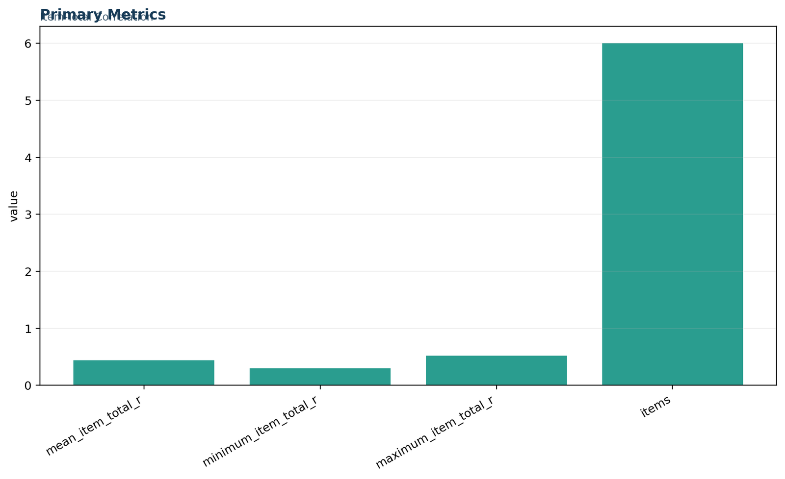
Primary metrics
Each item total correlation is shown beside its item mean. Famrel has the largest coefficient, while goout has the smallest.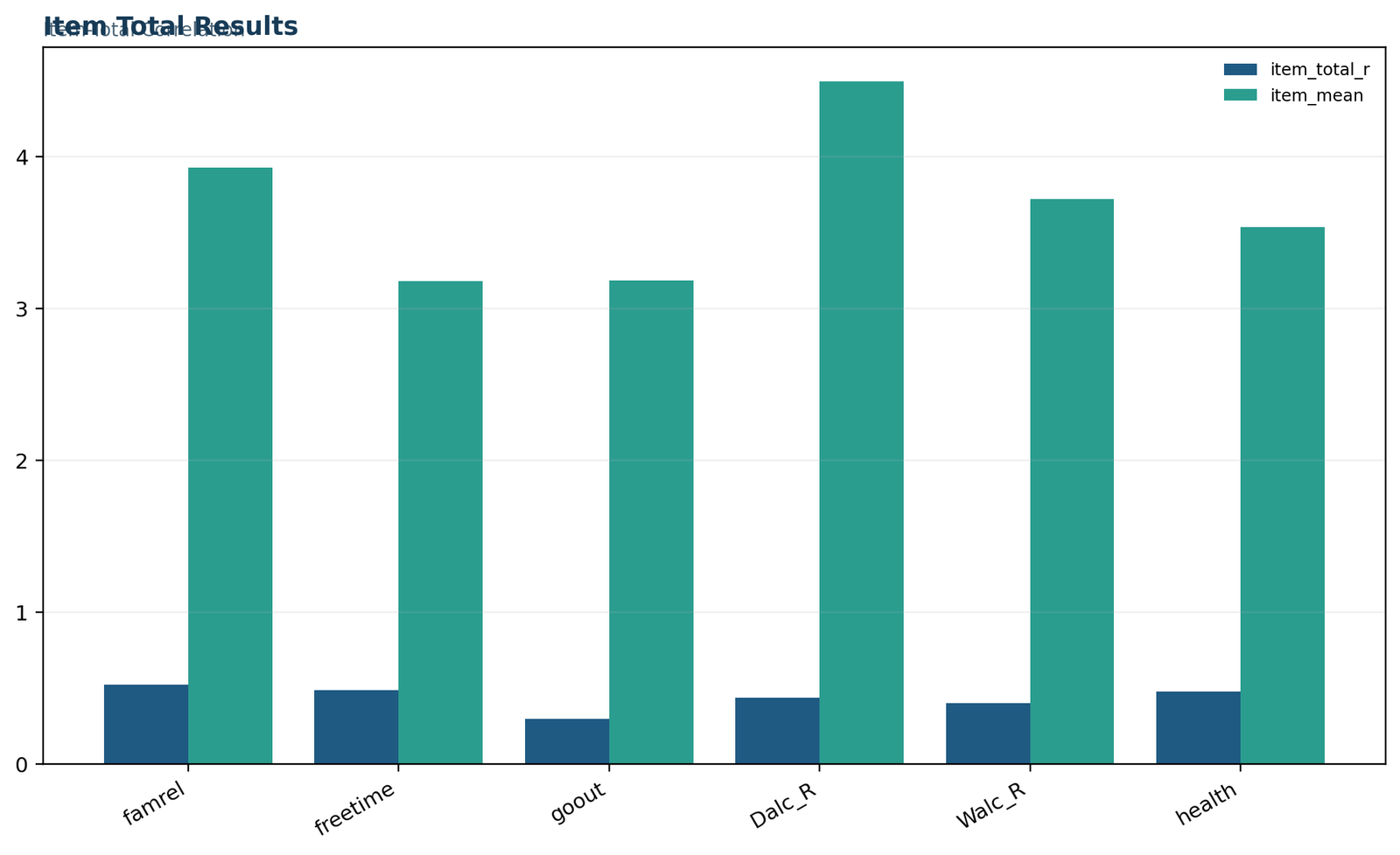
Item-level results
The composite includes 649 scores, with mean 22.0493, standard deviation 2.9696, minimum 12, median 22, and maximum 29.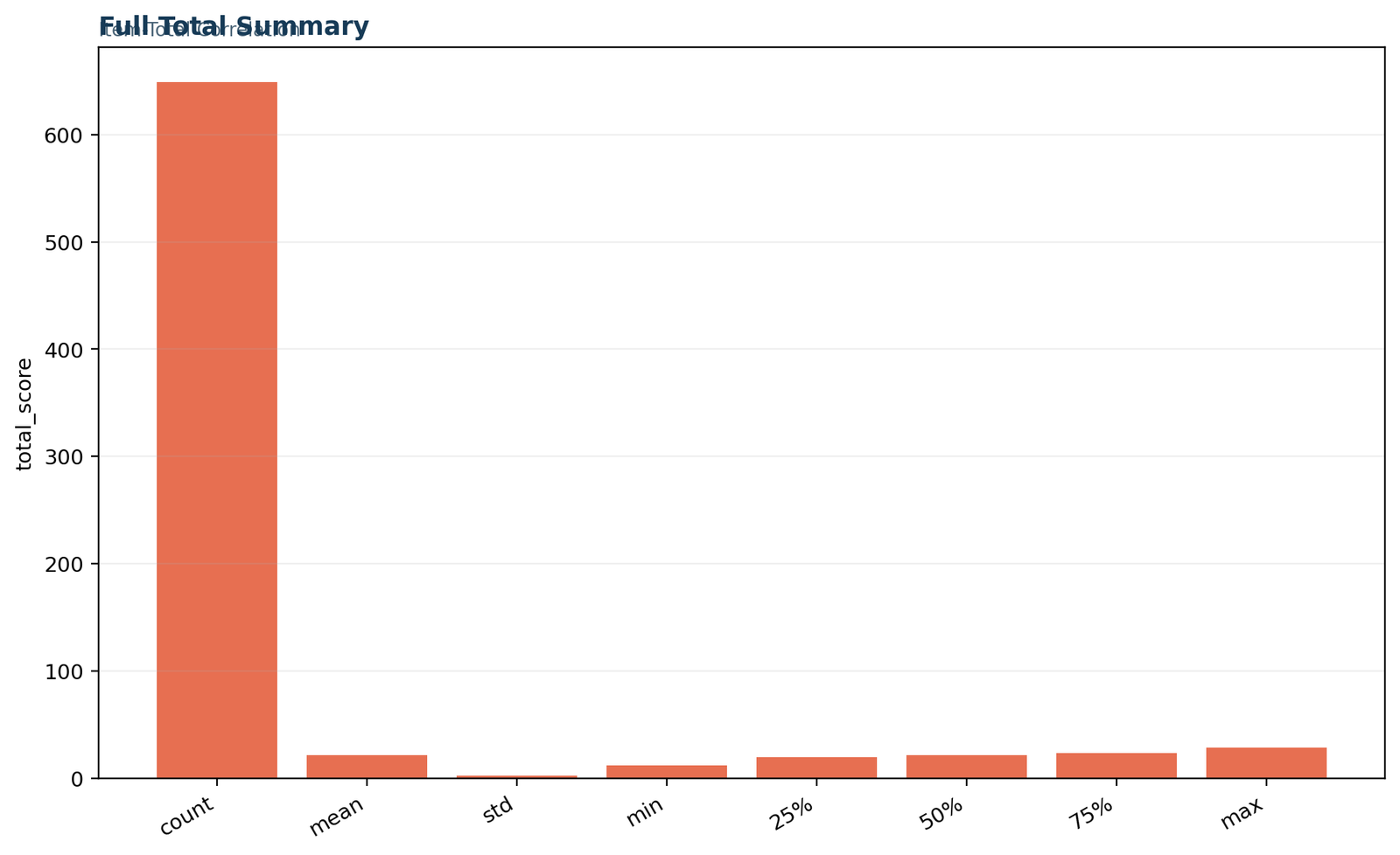
Full-total summary
The sorted order is famrel, freetime, health, Dalc_R, Walc_R, and goout. Item means are displayed as a separate descriptive series.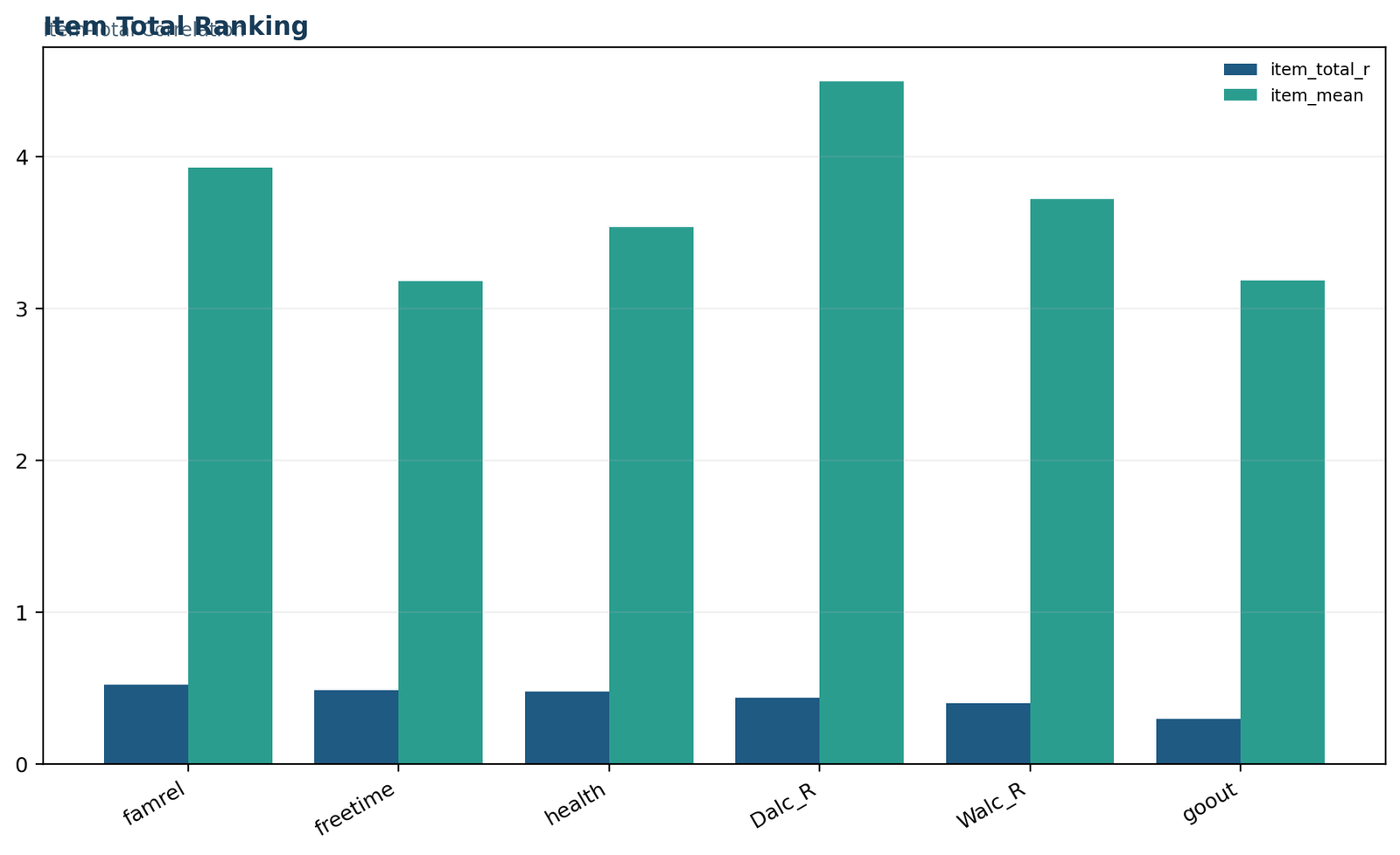
Ranking of items
The summary confirms agreement between calculated and reference values for the mean, minimum, maximum, and item count.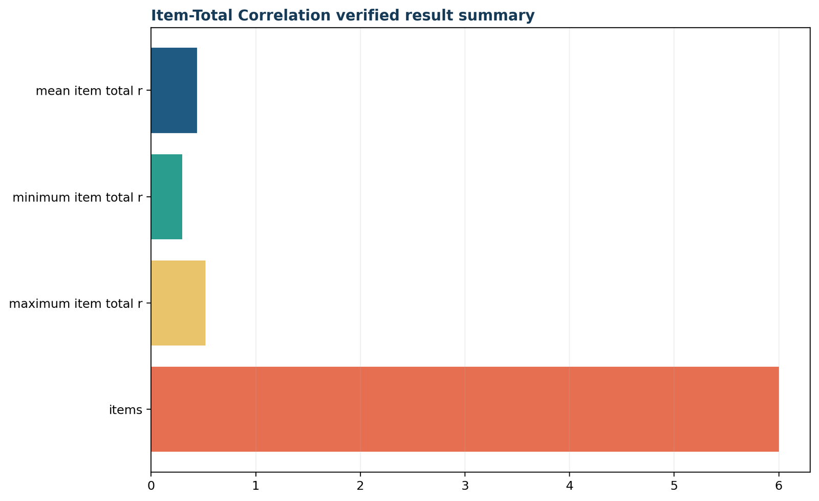
Verified result summary
Item total correlation in R: complete results and charts
The R workflow reproduces the same totals, rankings and corrected comparisons.
The item total correlation in R section uses the same six-item definition and 649 valid rows as Python. Identical numerical results across independent implementations provide an important reproducibility check.
The R analysis uses the same transformed variables, the same 649 rows, the same full_total definition, and the same Pearson coefficient. Its reported mean item total correlation is 0.436856224455792, the minimum is 0.295281303932179, and the maximum is 0.520485089194543. The tiny differences in the final decimal positions are ordinary floating-point display differences, not analytical disagreement. The correlation in R guide explains related correlation workflows.
R preserves the intended part-whole design: each item remains inside the full six-item total. That statement matters more than the software name. If an R function silently creates an item-rest total while a Python script uses the full total, the resulting tables will differ even though both calculations are internally correct. Reproducibility depends on matching the definition, not merely matching the variable names.
The R chart set recreates the same five evidence views. Agreement across software provides a strong computational cross-check because the coefficient table, full-total distribution, ranking, and summary metrics all converge. It does not, however, convert a broad six-item composite into a unidimensional scale; interpretation still depends on item content and the corrected statistics.
R reproduces the mean, minimum, maximum, and six-item count shown in the verified metric ledger.Primary metrics in R
The coefficient pattern matches Python: famrel is highest at 0.520485 and goout is lowest at 0.295281.Item-level R results
The full score distribution matches the independently produced Python and Excel summaries for all 649 records.R full-total summary
The rank order remains stable across implementations, supporting a direct software cross-check.R ranking
The final panel confirms exact agreement to the displayed precision across the metric ledger.R verified summary
Item total correlation in SPSS: reliability and correlation output
SPSS provides the full-total Pearson table and the corrected Item-Total Statistics table.
The item total correlation in SPSS workflow shows 649 valid cases, the full-total correlation matrix, item descriptives, Cronbach’s alpha, corrected item-total correlations, squared multiple correlations and alpha-if-deleted values.
SPSS can reproduce the full-total item correlation by first computing the transformed variables and full_total, then requesting a Pearson correlation matrix containing full_total and the six items. The output shows N = 649 for every pair and reports p < .001 for each item-to-full-total coefficient. For broader menu and output guidance, see correlation in SPSS.
The SPSS correlation table reports famrel = 0.520, freetime = 0.488, goout = 0.295, Dalc_R = 0.438, Walc_R = 0.402, and health = 0.478 after standard rounding. These values match the higher-precision Python, R, and Excel results. The table therefore verifies the primary item total correlation analysis directly.
SPSS RELIABILITY produces a different column labeled “Corrected Item-Total Correlation.” That column contains 0.227, 0.151, -0.105, 0.139, -0.033, and -0.010 for the six items. These are item-rest correlations, not the full-total coefficients. SPSS also reports Cronbach’s alpha = 0.112, standardized alpha = 0.169, and six items. The low alpha is consistent with the weak and negative corrected correlations.
The SPSS scale summary gives a mean of 22.0493, variance of 8.819, and standard deviation of 2.96960. Item means and standard deviations also match the independent outputs. One subtitle warning appears because the supplied subtitle exceeded SPSS’s 60-character limit and was truncated. That display warning does not affect the data, correlations, or reliability statistics.
Item total correlation in Excel: worked formulas and audit trail
The workbook exposes the scoring, totals and item-level calculations cell by cell.
The item total correlation in Excel workbook is useful when the analyst needs a visible audit trail. Each transformed item, the full total and the Pearson correlation can be checked directly rather than relying on a black-box summary.
The worked Excel file contains separate Guide, Data_Input, Working, Calculations, Diagnostics, and Reporting sheets. This structure keeps raw values, transformations, formula checks, and final reporting distinct. The correlation in Excel guide provides additional spreadsheet context, while the downloadable workbook below contains the exact worked example.
In the Working sheet, each row contains the six aligned items and a Full total column. The total is the row-wise sum of famrel, freetime, goout, Dalc_R, Walc_R, and health. The item total correlation for each variable is then calculated between its 649 values and the 649 full totals. The workbook’s famrel check returns 0.5204850891945386, matching the verified reference to floating-point precision.
The Calculations sheet records six items, the full-total variance of 8.818552759230732, and the final metric ledger. The Reporting sheet compares workbook results against verified references and shows an absolute difference of zero for the mean, minimum, maximum, and item count. The Diagnostics sheet states the key scope limitation: the target item intentionally remains in the full total.
A spreadsheet is especially useful for teaching because every row contribution remains visible. It also creates risks: copied formulas can shift ranges, text-formatted numbers may be ignored, blank cells may change the effective sample, and an analyst may accidentally correlate an item with a corrected rather than full total. Clear sheet separation and a visible row-count check reduce those risks.
How to interpret item total correlation responsibly
Magnitude, sign and scoring design must be interpreted together.
Item total correlation interpretation should begin with the sign, then consider magnitude, variation, content and whether the coefficient is corrected. Fixed cutoffs can be useful screening guides, but they cannot replace substantive judgment or dimensionality analysis.
There is no universal item total correlation cutoff that is valid for every scale, sample, and scoring design. Values around 0.30 are sometimes used as a rough screening reference, while values around 0.40 or 0.50 may be described as moderate or strong. Those labels are conventions, not laws. They are particularly risky for the uncorrected coefficient because part-whole overlap raises the value.
In the worked example, five full-total coefficients exceed 0.40 and goout is approximately 0.295. A superficial cutoff rule would suggest that most items perform acceptably. The corrected results show why that conclusion would be premature: no item reaches 0.30 against the rest score, and three corrected coefficients are negative. The full-total values are useful descriptive statistics, but they do not support a claim of strong internal consistency.
Interpretation should answer four questions. First, is the coefficient positive or negative? Second, how large is it in the context of the item’s variance and scale length? Third, does the corrected coefficient tell the same story? Fourth, does the item content plausibly belong to the same construct as the other items? A coefficient becomes meaningful only when all four questions are considered together.
Statistical significance should be treated separately from practical magnitude. With N = 649, even modest correlations can yield very small p-values. A p-value tests compatibility with a zero-correlation null model; it does not establish that the item is useful, unbiased, reliable, or substantively important. The coefficient itself is an effect-size measure of linear association, and its practical meaning depends on the measurement purpose.
Item total correlation and related reliability evidence
Cronbach’s alpha and item-total statistics answer related but different questions.
A sound reliability review combines item total correlation with corrected item-total correlations, inter-item correlations, alpha-if-deleted values and the conceptual role of each item. No single statistic should determine whether an item belongs in a composite.
Item total correlation and Cronbach’s alpha are related but not interchangeable. Item total correlation is item-specific: it describes one item’s association with a stated total. Alpha is scale-level: it summarizes the covariance structure of all items under assumptions that may not fit a multidimensional set.
The SPSS output reports alpha = 0.112 and standardized alpha = 0.169. Those values are low because several inter-item associations are negative or weak. For example, goout correlates -0.389 with Walc_R and -0.245 with Dalc_R, while Dalc_R and Walc_R correlate 0.617. The set contains clusters of behavior rather than a uniformly coherent single dimension.
An item can have a moderate uncorrected item total correlation even when alpha is low. This occurs because the item is included in the total, guaranteeing a self-variance contribution. Therefore, the positive full-total coefficients in this analysis do not conflict with low alpha. They answer a different mathematical question.
“Alpha if item deleted” is also not a standalone deletion rule. SPSS reports the highest value, 0.234, when goout is deleted, but that value remains low and the content of the composite changes. Item deletion should be based on construct definition, corrected item-total results, dimensionality, wording quality, and the purpose of scoring—not on whichever deletion produces the largest alpha.
Diagnostics, deeper interpretation and common mistakes
Most serious errors come from scoring, total construction or overinterpretation.
The most important item total correlation diagnostics are direction checks, range checks, scatterplots, missing-data verification, corrected comparisons and item-content review. Common errors include mixing full totals with item-rest totals and treating significance as practical adequacy.
1. Calling a corrected value uncorrected
Software often labels the item-rest coefficient as “corrected item-total correlation.” Confirm whether the target item was subtracted from the total before naming the statistic.
2. Forgetting reverse scoring
An item that points in the opposite direction can create a negative coefficient and depress reliability. Reverse first, then recompute the total from the transformed items.
3. Treating p < .05 as item quality
A significant correlation can still be too small or conceptually irrelevant. Large samples make small associations statistically detectable.
4. Using a universal 0.30 rule
Thresholds depend on whether the statistic is corrected, the number of items, construct breadth, response variance, and the measurement purpose.
5. Ignoring item variance
Ceiling or floor concentration can limit correlation. Review item means, standard deviations, and response frequencies before blaming wording or content.
6. Assuming high correlation proves validity
An item can correlate highly because it is redundant, shares wording, or is mathematically included in the total. Validity requires evidence beyond association.
7. Mixing missing-data rules
Python, R, SPSS, and Excel can use different rows unless missingness is handled explicitly. Always verify N and row lineage.
8. Reporting rounded values only
Publication tables may use three decimals, but verification files should preserve additional precision so implementations can be compared reliably.
Another mistake is interpreting the item total correlation as the percentage contribution of an item to the total. A coefficient of 0.52 does not mean the item contributes 52% of the composite score. The coefficient describes standardized linear co-movement, and the item is already part of the total. Score contribution is determined by the scoring rule, while correlation describes association across respondents.
Analysts also sometimes delete the lowest-ranked item without reviewing content. In this example, goout ranks last, but deletion would change the construct represented by the composite. Statistical screening should identify questions for review, not replace theoretical judgment. An item may be retained because it covers essential content even when its coefficient is modest.
A useful way to understand item total correlation is to separate three layers of meaning. The first layer is arithmetic: the item is part of the total, so a positive self-variance term is present. The second layer is empirical: respondents with higher scores on the item may also have higher totals because the item shares content or behavior with other components. The third layer is substantive: the analyst decides whether that observed pattern supports the intended use of the score. Confusing these layers leads to overinterpretation.
The arithmetic layer is fixed by formula. Even if an item is unrelated to the other items, it may retain a positive correlation with the full total because it contributes directly to that total. The size of the effect depends on the item variance, the variance of the remaining sum, and the covariance between the item and the rest. A high-variance item can have a noticeable full-total coefficient even when the rest-score relationship is weak.
The empirical layer depends on the sample. Item distributions may differ across age groups, institutions, cultures, administrations, or time periods. A coefficient obtained in one sample is not a permanent property of the item. Replication should use the same wording and scoring while also testing whether the item-total pattern changes across relevant groups. A stable item should not be assumed without evidence.
The substantive layer depends on the scoring model. A reflective scale assumes that items are manifestations of an underlying construct and should generally covary. A formative index combines components that may be distinct but jointly define an overall quantity. Internal consistency is central to the first case and may be less appropriate in the second. Before applying a cutoff, the analyst must decide which kind of score is being built.
The six-item example is broad: family relationships, free time, social outings, weekday alcohol behavior, weekend alcohol behavior, and health are not interchangeable indicators. Their low alpha and mixed corrected correlations are therefore understandable. The composite can still be calculated for a defined descriptive purpose, but it should not be described casually as a single highly reliable latent scale. The item total correlation table helps document how each component participates in the chosen sum.
Ranking also requires care. Famrel ranks first because its full-total coefficient is highest, not because it is the “best” item in every sense. Health ranks third in the full-total table but has a corrected coefficient near zero. Dalc_R and Walc_R share a relatively strong inter-item relationship because they represent related behaviors, yet their relationships with social and health variables are mixed. A one-dimensional rank cannot summarize all those patterns.
The mean item total correlation of 0.436856 is a summary of six coefficients. It is not the same as the average inter-item correlation, and it should not be inserted into formulas designed for the latter. The mean full-total value is partly driven by self-overlap for every item. When reliability theory requires average covariance or average inter-item correlation, those quantities must be calculated directly from item pairs.
Confidence intervals can be useful when item total correlations are compared across samples, but they require careful attention to dependence because the item and total share data and the coefficients are computed from the same respondents. Bootstrap procedures can provide empirical intervals, yet the resampling design should reflect clustering or repeated measures when present. This worked report focuses on exact point estimates verified across software rather than adding unsupported interval calculations.
Nonlinearity is another consideration. Five-category items create horizontal bands in a scatterplot against the total. Pearson correlation still provides a familiar standardized summary, but it cannot reveal all distributional features. Grouped total means by item category, box plots, and category frequencies can show whether the relationship is monotonic, whether one category behaves unexpectedly, or whether sparse categories make the coefficient unstable.
Ties are unavoidable with ordinal response scales. Spearman correlation may be considered when the goal is monotonic rank association, while polychoric methods may be considered under latent-variable assumptions. Those alternatives answer slightly different questions and should not be substituted silently. If the reported statistic is called item total correlation and the analysis plan specifies Pearson’s r, the software should reproduce that definition exactly.
Missing data can alter both the item and the total. If the total is calculated only for complete rows, the analysis may exclude respondents with any missing item. If totals are prorated, different respondents can have totals based on different item counts, changing the meaning of the score. Pairwise correlation can also produce a different N for each item. The present example avoids that ambiguity because all six variables are complete for 649 records.
Reverse scoring should be verified with observed minima and maxima. For a 1-to-5 item, the transformation 6 − X maps 1 to 5, 2 to 4, 3 to 3, 4 to 2, and 5 to 1. A mistaken constant such as 5 − X would create values from 0 to 4 and shift the total. A mistaken reversal after total creation would leave the composite inconsistent. Documentation should name both the original and transformed variables.
The precision of the cross-software agreement is valuable. Python reports 0.4368562244557915 for the mean; R reports 0.436856224455792. The difference is below the meaningful display precision and reflects binary floating-point representation and formatting. Excel reproduces the same ledger, while SPSS rounds the visible correlation matrix to three decimals. The convergence indicates that the analytical definition was implemented consistently.
Verification does not mean every chart is equally informative. A chart that places “items = 6” beside correlations below 1 uses a shared axis with unlike units, so the count dominates visually. A chart that places item means around 3 to 4.5 beside correlations around 0.3 to 0.5 similarly emphasizes the means. Those panels remain useful as compact dashboards, but exact-value tables should guide comparisons.
A publication-quality discussion should therefore move from definition to verification to interpretation. First define the total and formula. Then show exact coefficients and software agreement. Next compare corrected values, item distributions, and reliability. Finally discuss whether the composite is being used as a broad index or a reflective scale. That sequence prevents a single attractive coefficient from carrying more meaning than it can support.
How to report item total correlation in APA style
State the total definition, sample size, coefficient type, exact values and corrected comparison.
An APA-style item total correlation report should identify the six-item composite, explain that the target item remained in the full total, report N and the coefficient range, and distinguish the corrected item-total findings from the uncorrected values.
A complete report should identify the coefficient, the total-score definition, the item transformations, the sample size, the exact results, and the interpretive limitation. The phrase “item total correlation” alone is insufficient because readers may assume a corrected item-rest statistic.
A more interpretive statement can add that corrected item-total correlations ranged from -0.105 to 0.227 and that alpha was 0.112. This comparison demonstrates that the six-item composite has positive part-whole associations but weak internal consistency as a single scale. The wording should remain neutral: the analysis does not prove that the items are defective, only that they do not behave as a strongly homogeneous set under this reliability model.
Report exact p-values where software provides them, but use “p < .001” instead of “p = .000.” The hypothesis-testing guide explains why a probability is not literally zero. Include a results table with item names, full-total correlations, corrected correlations, item means, and N so readers can distinguish statistical definitions without searching through software output.
Item total correlation PDF, Excel and software downloads
Use the verified files to inspect calculations and reproduce the analysis.
The downloadable item total correlation resources include the Python report, R report, SPSS output and worked Excel workbook. Together they provide a cross-platform record of the same scoring design and exact results.
R PDFIndependent R calculation using the identical full-total design.Open report →
SPSS PDFCorrelation matrix, reliability output, item statistics, and scale summary.Open output →
Worked ExcelData input, transformations, calculations, diagnostics, and reporting ledger.Open workbook →
Technical workflow, applications and reproducibility notes
A documented sequence protects the analysis from silent scoring changes.
The technical item total correlation workflow records reverse scoring, valid rows, total construction, coefficient calculation, corrected comparison, software reconciliation and reporting. The same process applies to questionnaires, educational tests, rubrics and other composite scores.
A reproducible item total correlation analysis should make every scoring decision visible. The following workflow mirrors the verified Python, R, SPSS, and Excel outputs and avoids the common mistake of silently switching between a full total and an item-rest total.
Confirm item direction
List the meaning of high and low values. Reverse-score items whose original direction conflicts with the intended composite. In this example, Dalc_R = 6 − Dalc and Walc_R = 6 − Walc.
Check valid rows
Verify the number of cases contributing to each coefficient. The worked analysis retains 649 complete records, and every reported coefficient uses N = 649.
Create the full total
Sum famrel, freetime, goout, Dalc_R, Walc_R, and health for each record. Do not subtract the target item because this analysis is intentionally uncorrected.
Correlate each item with the full total
Calculate six Pearson correlations: one between each item and full_total. Retain enough decimal places for verification, then round consistently for publication.
Rank and summarize
Order coefficients from largest to smallest, calculate the mean, minimum, and maximum, and inspect item means so restricted ranges are not overlooked.
Compare with item-rest results
Where item-retention decisions are planned, also calculate corrected item-total correlations. The comparison reveals how much the shared item contributes to the full-total coefficient.
Report design and limitations
State explicitly that the item remains in the total. Describe sample size, coding transformations, coefficient type, and the distinction from corrected item-total correlation.
This sequence is software-neutral. Different programs may format tables differently, but the verified values must agree when the same rows, transformations, total-score definition, and Pearson formula are used. A mismatch almost always comes from a data-selection difference, missing-value rule, reverse-scoring error, or use of the corrected rather than uncorrected statistic.
In educational testing, item total correlation can identify questions that move with overall test performance. For right/wrong items, the statistic is closely related to item discrimination, although specialized point-biserial methods are often used. In rating scales, it summarizes how each response category score aligns with the composite.
In survey development, item total correlation can reveal reverse-keying errors and items with weak alignment. A researcher might calculate the full-total version for descriptive replication and the corrected version for item screening. The two columns should be displayed together when stakeholders could otherwise confuse them.
In operational dashboards, the statistic can compare the behavior of component indicators within an index. Because components may represent intentionally different domains, a modest corrected correlation may be acceptable. The goal of a multidomain index is not always internal homogeneity. That decision depends on whether the total is intended as a latent scale, a formative index, or a practical summary.
In health and psychological measurement, stronger evidence is usually required before retaining or deleting items. Factor structure, test-retest stability, measurement invariance, content validity, criterion relationships, and response-process evidence can all matter. Item total correlation is a diagnostic, not a complete validation study.
Across applications, the best practice is the same: define the score, preserve the item wording and coding map, show the sample size, distinguish full-total from item-rest calculations, and interpret the coefficient in the context of the measurement purpose.
Item total correlation FAQs
Answers to practical questions about formulas, cutoffs, corrected coefficients and software.
These item total correlation FAQs address the distinctions most likely to affect an actual analysis: whether the item belongs in the total, why corrected values differ, how negative coefficients arise and how to report results without overclaiming.
What is item total correlation?
Item total correlation is the Pearson correlation between one item and a composite total score that includes that same item. It measures part-whole linear association. A positive value means higher item scores tend to occur with higher totals; a negative value means the item tends to move against the total. Because the item is mathematically contained in the total, the coefficient is generally larger than a corrected item-total correlation.
What is the formula for item total correlation?
The formula is r_i,T = cor(X_i, T), where X_i is the target item and T is the sum of all items, including X_i. In covariance form, r_i,T = Cov(X_i,T) divided by SD(X_i) times SD(T). The corrected formula instead uses cor(X_i, T − X_i).
What is a good item total correlation?
There is no universal cutoff. Values near .30, .40, or .50 are sometimes used as rough descriptors, but the uncorrected statistic is inflated by part-whole overlap. A responsible interpretation reports the exact coefficient, the total definition, item variance, corrected item-total correlation, scale purpose, and content relevance rather than relying on one threshold.
What is an acceptable item-total correlation range?
The mathematical range is -1 to +1. In practice, positive coefficients are generally expected when items share a scoring direction. A value around .30 may be used as a preliminary reference in some settings, but that rule is more often applied to corrected item-total correlations. Uncorrected values should not be judged with a mechanical universal cutoff.
What is the difference between item total correlation and corrected item-total correlation?
Item total correlation uses the full total that includes the target item. Corrected item-total correlation removes the item before creating the comparison score. The corrected statistic therefore measures association with the remaining items and avoids direct self-overlap. In this example, famrel changes from .520 uncorrected to .227 corrected.
Why is item total correlation usually positive?
The item is part of the total, so its own variance contributes positively to the covariance with that total. This mathematical overlap can make a full-total coefficient positive even when the item has little or negative association with the remaining items. The goout result illustrates this: .295 uncorrected but -.105 corrected.
What does a negative item total correlation mean?
A negative value means higher item scores tend to accompany lower composite totals. Possible explanations include a reverse-keying error, inconsistent scoring direction, ambiguous wording, a different construct, subgroup effects, or data problems. The analyst should review coding and content before deleting the item.
Can item total correlation exceed 1?
No. Like any Pearson correlation, a correctly calculated item total correlation lies between -1 and +1. A value outside that interval indicates a calculation, formatting, or data error. Item means, covariances, regression coefficients, and reliability statistics can use other scales, so confirm that the reported column is actually a correlation.
Should the item be included in the total?
It depends on the statistic intended. Include the item when the goal is the uncorrected part-whole item total correlation. Exclude it when the goal is corrected item-total or item-rest correlation. For item-retention decisions, the corrected version is usually more informative because it avoids self-overlap.
How do I calculate item total correlation in SPSS?
Create any required reverse-scored items, compute the full composite, and request Pearson correlations between full_total and each item. The resulting item-to-full_total cells are the uncorrected item total correlations. The SPSS RELIABILITY table labeled Corrected Item-Total Correlation reports item-rest values instead.
How do I calculate item total correlation in Excel?
Place aligned items in columns, calculate a row sum for the full total, and use the Pearson correlation function between each item column and the full-total column. Verify that all ranges cover the same rows and that the item remains in the total. Preserve a row-count check and compare results with a reference ledger.
How do I calculate item total correlation in R?
After reverse scoring and creating the full row sum, calculate a Pearson correlation between each item vector and the full-total vector. Ensure that missing-data handling is identical for every item and that the total includes the target item. Label the result clearly so it is not mistaken for an item-rest coefficient.
How do I calculate item total correlation in Python?
Create transformed item columns, sum them row by row, and calculate Pearson correlations between each item and the full total. Confirm N, retain full precision in the verification output, and present rounded values in the public table. The exact worked outputs are available in the downloadable Python report.
Is item total correlation the same as item discrimination?
They are related but not always identical. In classical test theory, item-total or point-biserial associations are often used as discrimination indicators. The exact statistic depends on whether the item is binary or polytomous, whether the total is corrected, and how the score is defined. Always report the specific coefficient used.
Does a high item total correlation prove validity?
No. A high coefficient shows association with the stated total in the observed sample. It can reflect shared wording, redundancy, common method variance, or part-whole overlap. Validity requires broader evidence about content, internal structure, relationships with other variables, response processes, fairness, and consequences of score use.
Why are corrected correlations lower than full-total correlations?
Corrected correlations remove the target item from the total. The full-total coefficient contains the item’s own variance, which directly increases covariance with the total. Once that self-contribution is removed, only the relationship with the remaining items remains. Large drops are therefore expected when inter-item coherence is weak.
What does p < .001 mean for an item total correlation?
It means the observed coefficient would be unlikely under a model with zero population correlation, given the assumptions and sample size. It does not mean the item is important, valid, or reliable. With 649 observations, even moderate coefficients are highly significant, so magnitude and measurement context deserve more attention.
Can I delete the item with the lowest correlation?
Do not delete an item automatically. Review scoring, wording, content coverage, variance, corrected correlation, dimensionality, and the effect on the intended construct. The lowest item may measure an essential domain. Statistical screening identifies items for investigation; it does not make the final content decision.
How many decimal places should I report?
Three decimals are usually readable in a results table, while four to six may be useful for technical verification. Use the same rounding rule throughout. Keep full precision in analysis files so Python, R, SPSS, and Excel outputs can be compared without mistaking rounding differences for computational disagreement.
What did the worked example find?
Across 649 records and six aligned items, the mean item total correlation was .436856, the minimum was .295281 for goout, and the maximum was .520485 for famrel. All full-total coefficients were positive and had p < .001. Corrected coefficients were much lower, and Cronbach’s alpha was .112, indicating weak homogeneity.
Related statistical guides
Continue with reliability, correlation and descriptive-statistics resources.