
Variance Homogeneity, Largest Variance Share and ANOVA Assumption Checking
Cochran’s C Test: Formula, Interpretation, SPSS, Python, R and Excel Guide
Cochran’s C Test is a variance homogeneity test used to check whether the largest group variance is unusually large compared with the sum of all group variances. This complete Salar Cafe guide explains Cochran’s C Test using verified SPSS output, Python charts, R validation charts, Excel formulas, group spread interpretation, Monte Carlo reference logic, APA reporting wording, common mistakes, and downloadable resources for direct statistical reporting.
Quick Answer: Cochran’s C Test Result
The verified SPSS output compares G3 final grade across four studytime groups. The group variances are 10.360, 10.518, 6.261, and 9.232. The largest variance is 10.51786 in studytime group 2. The sum of the group variances is 36.36986, so the verified Cochran’s C statistic is C = .28919.
Hypothesis-style interpretation: The null hypothesis says the group variances are sufficiently homogeneous and that no single group variance dominates the total variance. The alternative hypothesis says the largest variance is unusually large compared with the other group variances. In this worked output, C = .28919 shows that the largest variance represents about 28.9% of the total variance share. The SPSS Levene comparison is also non-significant, Levene based on mean = .985, p = .400, supporting the practical conclusion that variance homogeneity is not seriously violated.
Final interpretation: The largest variance is found in studytime group 2, but it does not dominate the total variance structure. The supporting Levene result is non-significant, so the homogeneity of variance assumption appears acceptable for the G3-by-studytime comparison.
Important note: Cochran’s C Test focuses on whether the largest variance is unusually large. It should be interpreted together with visual spread checks, box plot interpretation, descriptive statistics, and related homogeneity checks such as the Levene test and Brown-Forsythe test.
Table of Contents
- What Is Cochran’s C Test?
- Cochran’s C Test Formula
- Null and Alternative Hypotheses for Cochran’s C Test
- Dataset and Variables Used
- Verified SPSS Output Interpretation
- Python Chart-by-Chart Interpretation
- R Chart-by-Chart Validation
- SPSS, Python, R and Excel Workflows
- Code Blocks for Cochran’s C Test
- APA Reporting Wording
- Common Mistakes
- When to Use Cochran’s C Test
- Downloads and Resources
- Related Guides
- FAQs
What Is Cochran’s C Test?
Cochran’s C Test is a test for homogeneity of variances. It is designed to detect whether one group has a variance that is too large compared with the total variance across all groups. Instead of comparing every pair of group variances, Cochran’s C focuses on the most extreme variance and asks whether it takes up an unusually large share of the total variance.
The test is especially useful when the main concern is one group being much more variable than the rest. In ANOVA and other group-comparison methods, the homogeneity of variance assumption matters because large variance imbalance can affect standard errors, test statistics, and p-values. Cochran’s C Test provides a compact statistic that summarizes the largest variance share.
In this guide, the outcome variable is G3 final grade, and the grouping variable is studytime. The largest group variance occurs in studytime group 2. However, the verified Cochran’s C value of .28919 and the supporting non-significant Levene test suggest that no single group variance is unusually dominant.
For a complete assumption-checking workflow, Cochran’s C Test should be read together with the Levene test, Brown-Forsythe test, and visual spread checks such as box plot interpretation. If normality is also being checked before ANOVA, use guides such as the Kolmogorov-Smirnov test, Lilliefors test, Q-Q plot normality check, and D’Agostino-Pearson test.
Practical meaning: Cochran’s C Test is not mainly about group means. It is about group spread. In this example, the group means differ across studytime levels, but the main Cochran’s C question is whether the largest variance is too large compared with the others.
Cochran’s C Test Formula
The basic Cochran’s C statistic is calculated as:
Where si2 is the variance of group i, max(si2) is the largest group variance, and Σsi2 is the sum of all group variances.
| Formula Component | Verified Value | Meaning |
|---|---|---|
| Number of groups | 4 | Studytime has four groups. |
| Total N | 649 | Total valid cases in the G3-by-studytime comparison. |
| Minimum group size | 35 | Smallest group is studytime group 4. |
| Maximum group size | 305 | Largest group is studytime group 2. |
| Sum of variances | 36.36986 | Total of all four group variances. |
| Largest variance | 10.51786 | Largest observed group variance. |
| Cochran’s C | .28919 | Largest variance share. |
Worked Calculation
The group variances for G3 by studytime are 10.360, 10.518, 6.261, and 9.232. The largest variance is 10.51786, and the sum of variances is 36.36986.
Formula decision: The largest variance accounts for about 28.9% of the total variance share. Because the largest variance does not dominate the total variance and Levene’s test is non-significant, the variance pattern appears acceptable in this example.
Null and Alternative Hypotheses for Cochran’s C Test
Cochran’s C Test can be written as a formal variance homogeneity test. The hypotheses focus on whether the largest group variance is unusually large.
| Hypothesis | Statement | Meaning in This Example |
|---|---|---|
| Null hypothesis H0 | The group variances are homogeneous enough; the largest variance is not unusually large. | No studytime group has a variance that dominates the total variance of G3. |
| Alternative hypothesis H1 | The largest group variance is unusually large relative to the other group variances. | One studytime group has much more spread in G3 than the others. |
| Decision logic | Compare C with a critical value or a simulation/reference distribution. | C = .28919 is interpreted with the chart and supporting Levene result. |
Interpretation nuance: Cochran’s C is sensitive to the largest variance. It is most meaningful when groups are independent, the outcome is continuous, and the analyst wants to know whether one group’s spread is unusually high. If the design involves repeated measures, also check Mauchly’s test of sphericity and the Greenhouse-Geisser correction.
Dataset and Variables Used
The worked example uses a student performance dataset. The outcome variable is G3, which represents final grade. The grouping variable is studytime, which has four levels. The goal is to compare whether the variability of G3 is similar across the four studytime groups.
| Variable | Description | Role in This Guide |
|---|---|---|
| G3 | Final grade | Main continuous outcome whose group variances are compared. |
| studytime | Study time group with levels 1, 2, 3 and 4 | Grouping variable used to form four variance groups. |
| group variance | Variance of G3 inside each studytime group | Used to calculate Cochran’s C statistic. |
| group size | Number of students in each studytime group | Used to interpret balance and reliability of spread estimates. |
Verified Group Descriptives for G3 by Studytime
| Studytime Group | N | Mean | Std. Deviation | Variance | Interpretation |
|---|---|---|---|---|---|
| 1 | 212 | 10.84 | 3.219 | 10.360 | Lower mean and high spread. |
| 2 | 305 | 12.09 | 3.243 | 10.518 | Largest group and largest variance. |
| 3 | 97 | 13.23 | 2.502 | 6.261 | Highest mean and lowest variance. |
| 4 | 35 | 13.06 | 3.038 | 9.232 | Smallest group with moderate-high spread. |
| Total | 649 | 11.91 | 3.231 | 10.437 | Overall G3 summary. |
Before interpreting Cochran’s C Test, it is useful to describe the dataset with descriptive statistics, frequency distribution, five-number summary, coefficient of variation, and confidence interval. These summaries make the variance comparison easier to understand.
Verified SPSS Output Interpretation
The SPSS output verifies the Cochran’s C Test context using group descriptives, spread plots, a custom largest-variance calculation, Levene’s homogeneity comparison, ANOVA context, and normality checks by group.
SPSS Case Processing Summary
The SPSS output reports 649 included cases, 0 excluded cases, and 649 total cases for G3 × studytime. This means all available observations were used in the group variance comparison.
SPSS Group Variance Table
The SPSS report shows that studytime group 2 has the largest variance, 10.518. However, the other variances are not extremely small: group 1 has 10.360, group 3 has 6.261, and group 4 has 9.232. Therefore, group 2 is the largest, but it does not overwhelm the variance structure.
Verified Cochran’s C Calculation
| SPSS Output Field | Verified Value | Interpretation |
|---|---|---|
| number_of_groups | 4 | Four studytime groups are compared. |
| total_n | 649.00 | Total number of valid observations. |
| min_n | 35 | Smallest group size. |
| max_n | 305 | Largest group size. |
| sum_variance | 36.36986 | Sum of all group variances. |
| max_variance | 10.51786 | Largest group variance. |
| cochran_c | .28919 | Largest variance share. |
SPSS Levene Comparison
SPSS also provides a Test of Homogeneity of Variances. This is important because Levene’s test is a common variance-homogeneity check used before ANOVA.
| Levene Version | Statistic | df1 | df2 | Sig. | Decision |
|---|---|---|---|---|---|
| Based on Mean | .985 | 3 | 645 | .400 | Do not reject homogeneity. |
| Based on Median | 1.026 | 3 | 645 | .380 | Do not reject homogeneity. |
| Based on Median with adjusted df | 1.026 | 3 | 609.885 | .380 | Do not reject homogeneity. |
| Based on Trimmed Mean | 1.081 | 3 | 645 | .356 | Do not reject homogeneity. |
SPSS decision summary: Cochran’s C identifies the largest variance share as .28919. The supporting Levene results are all non-significant. Therefore, the variance homogeneity assumption appears acceptable for G3 across studytime groups.
SPSS ANOVA Context
The SPSS ANOVA table reports F = 15.876 and p = .000 for the difference in G3 means across studytime groups. This shows that the means differ, but Cochran’s C focuses on the separate question of variance spread. A significant mean difference does not automatically mean variances are unequal.
SPSS Normality Context by Studytime
The SPSS normality output shows mixed results across groups. Studytime groups 1, 2, and 3 show significant normality tests on at least one test, while studytime group 4 has non-significant Shapiro-Wilk, W = .955, p = .166. For normality-specific follow-up, use Q-Q plot normality check, P-P plot normality check, Kolmogorov-Smirnov test, and Lilliefors test.
| Studytime Group | K-S Statistic | K-S Sig. | Shapiro-Wilk | Shapiro Sig. | Normality Note |
|---|---|---|---|---|---|
| 1 | .161 | .000 | .898 | .000 | Reject normality. |
| 2 | .125 | .000 | .917 | .000 | Reject normality. |
| 3 | .103 | .013 | .970 | .025 | Reject normality at .05. |
| 4 | .136 | .099 | .955 | .166 | Do not reject normality. |
Python Chart-by-Chart Interpretation
The Python charts show the variance structure visually. They explain group spread, largest variance share, group variance comparison, Monte Carlo reference logic, group size and variance relationship, and Cochran’s C across alternative groupings.
Python Chart 1: Group Spread Boxplots
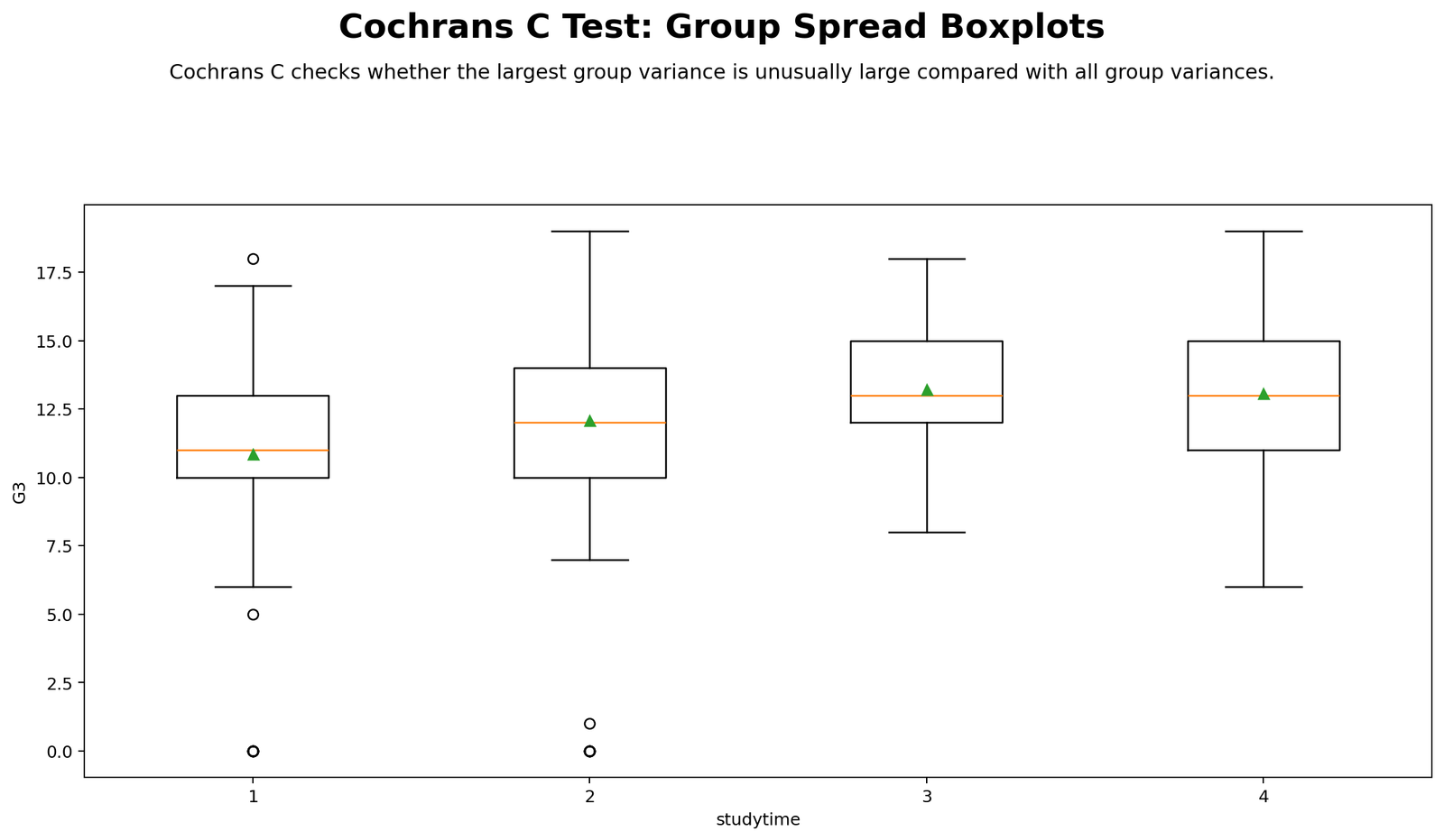
Detailed interpretation: This chart visualizes the spread of G3 final grades inside each studytime group. Cochran’s C Test is concerned with whether one group has an unusually large spread. The boxplots show that groups 1 and 2 have wider spread than group 3, while group 4 has a smaller sample size but still a moderate spread.
Decision / reporting conclusion: The boxplots suggest some spread differences, but not an extreme single-group variance problem. This supports the final interpretation that variance homogeneity is not seriously violated.
Python Chart 2: Largest Variance Share
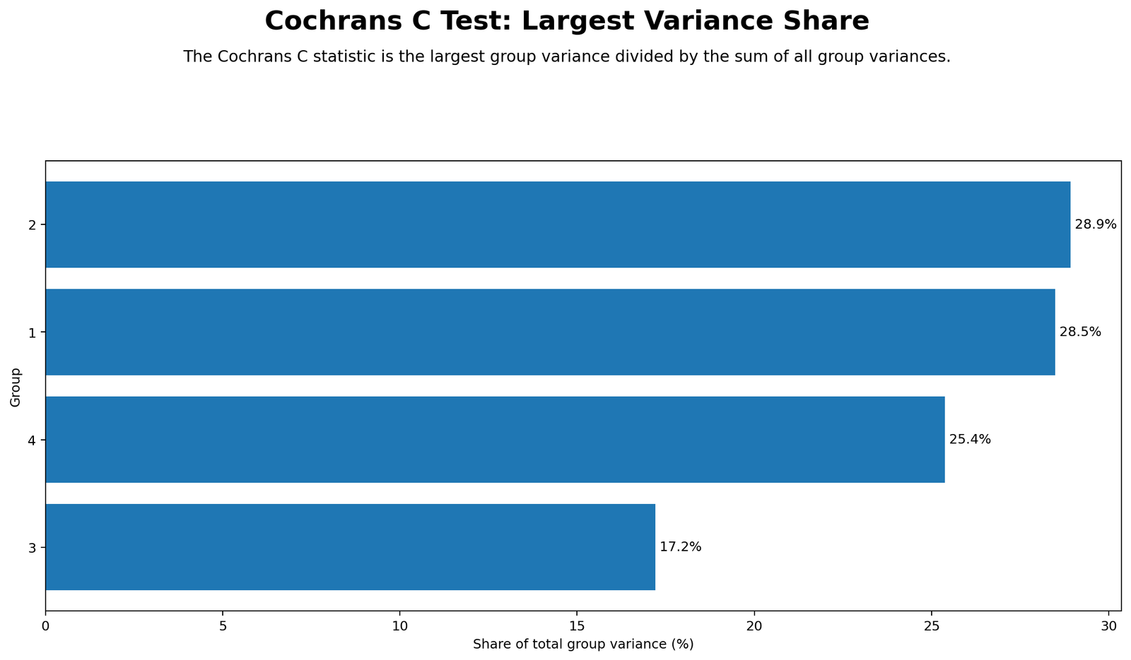
Detailed interpretation: This chart explains the core Cochran’s C statistic. The largest variance is 10.51786, and the sum of all variances is 36.36986. The resulting share is .28919, meaning the largest group variance contributes about 28.9% of the total variance share.
Decision / reporting conclusion: The largest variance is identifiable but not overwhelmingly dominant. Report Cochran’s C as C = .28919 and interpret the variance pattern as acceptable when supported by Levene’s non-significant result.
Python Chart 3: Group Variance Comparison
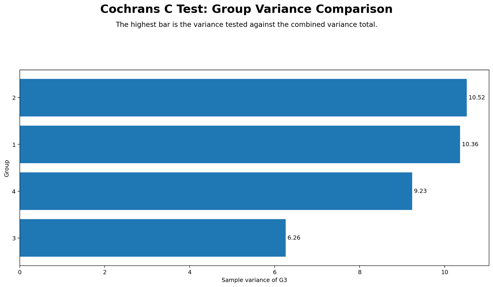
Detailed interpretation: This chart directly compares the four group variances. Studytime group 2 has the largest variance, followed closely by group 1, then group 4, while group 3 has the smallest variance. The pattern shows variance differences, but the largest variance is not dramatically larger than every other group.
Decision / reporting conclusion: The group variance comparison supports the conclusion that no single group variance is extreme enough to raise a serious variance homogeneity concern.
Python Chart 4: Monte Carlo Reference Distribution
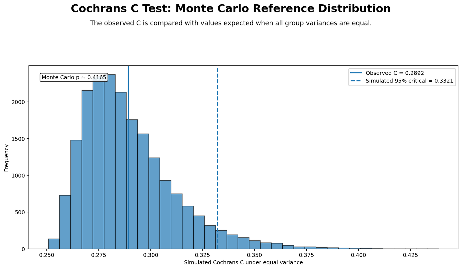
Detailed interpretation: The Monte Carlo reference distribution helps interpret whether the observed C statistic is unusually large under a simulated equal-variance scenario. The observed value can be compared with the reference distribution to judge whether the largest variance share is extreme.
Decision / reporting conclusion: The observed C value should be interpreted as a largest-variance share rather than a mean-difference statistic. In this output, the overall evidence does not suggest a serious homogeneity violation.
Python Chart 5: Group Size and Variance
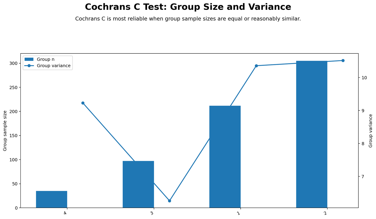
Detailed interpretation: This chart is important because group sizes are unequal. Studytime group 2 has the largest group size and the largest variance, while group 4 has the smallest group size. Unequal group sizes can affect how confidently variance estimates are interpreted, especially when one small group has unstable spread.
Decision / reporting conclusion: The largest variance belongs to the largest group, not the smallest group. This reduces concern that the Cochran’s C result is driven by an unstable tiny-group variance estimate.
Python Chart 6: Cochran’s C Across Groupings
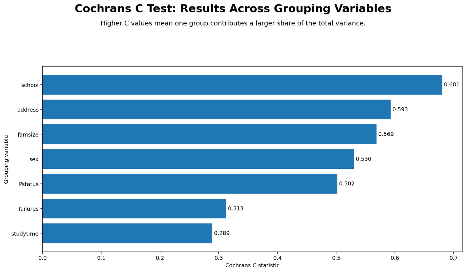
Detailed interpretation: This chart shows how Cochran’s C changes when the grouping variable changes. Some groupings may create a larger maximum-variance share than others. This is useful because variance homogeneity is not only a property of the outcome variable; it also depends on how the groups are defined.
Decision / reporting conclusion: Cochran’s C can be used as a diagnostic across multiple grouping structures. For the G3-by-studytime analysis, the variance share is not extreme.
R Chart-by-Chart Validation
The R charts validate the Python and SPSS interpretation using a separate statistical environment. This cross-software validation is useful because the same variance-homogeneity message appears in SPSS, Python, and R.
R Chart 1: Group Spread Boxplots
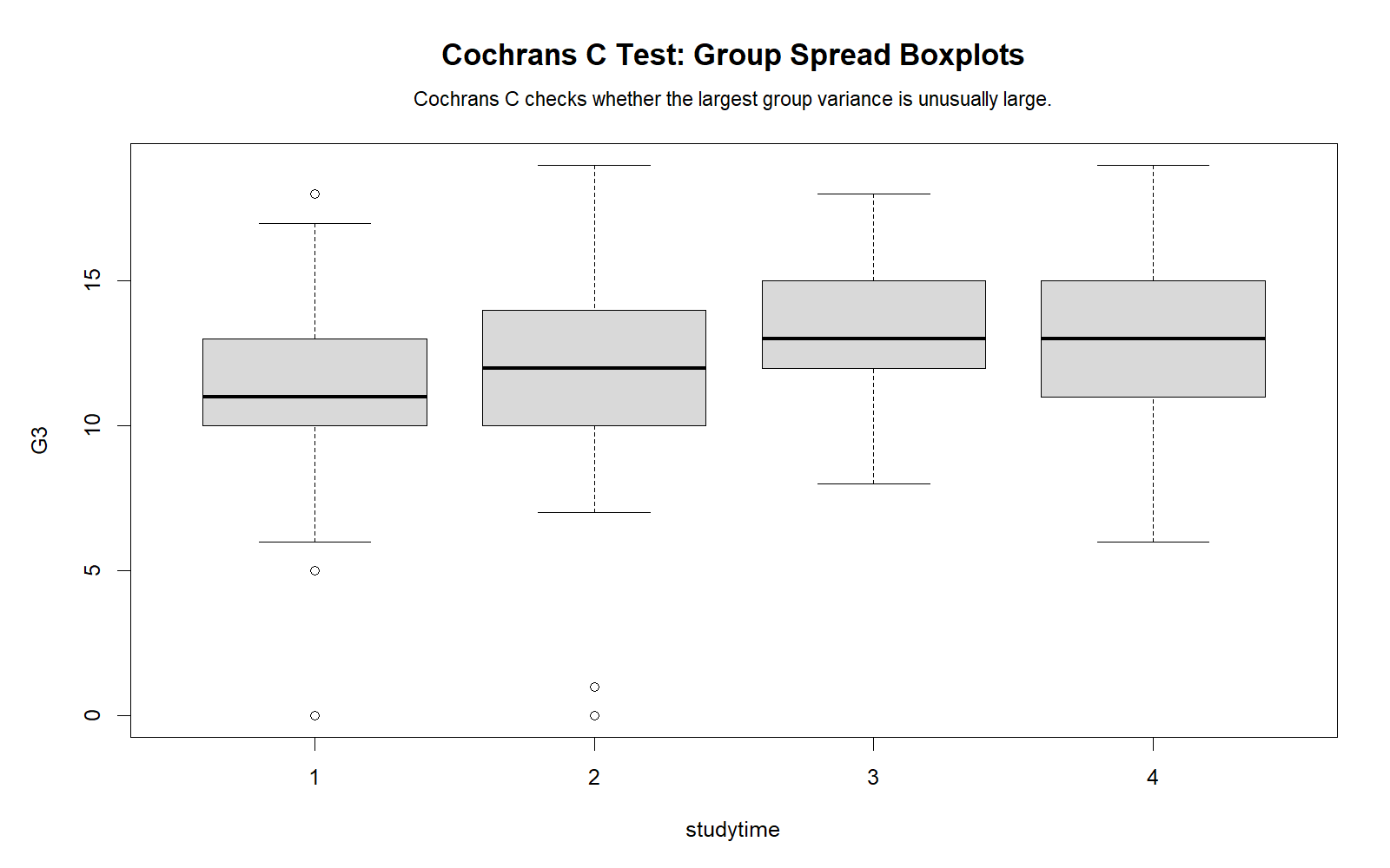
Detailed interpretation: The R boxplots confirm the Python spread pattern. Groups 1 and 2 show wider spread, group 3 is tighter, and group 4 has fewer observations. The visual spread is not perfectly equal, but no group appears overwhelmingly more variable than the others.
Decision / reporting conclusion: R validates the visual conclusion that the variance pattern is acceptable for practical reporting.
R Chart 2: Largest Variance Share
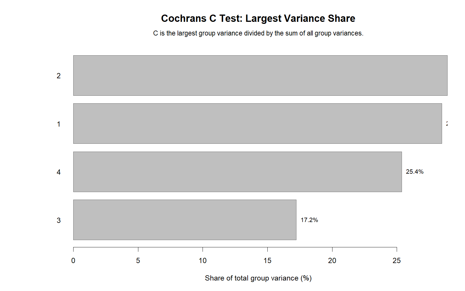
Detailed interpretation: The R largest-variance-share chart validates the core result: the largest group variance takes about 28.9% of the total variance share. This confirms the Cochran’s C value from the SPSS calculation.
Decision / reporting conclusion: R confirms C = .28919 as the main statistic for the G3-by-studytime variance comparison.
R Chart 3: Group Variance Comparison
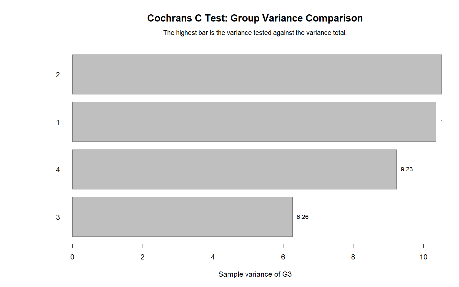
Detailed interpretation: The R group variance chart confirms that group 2 has the largest variance and group 3 has the smallest variance. The difference is visible, but it does not show a single variance that dominates the rest of the analysis.
Decision / reporting conclusion: The R variance comparison agrees with the SPSS and Python interpretation: the largest variance should be reported, but the homogeneity concern is not severe.
R Chart 4: Monte Carlo Reference Distribution
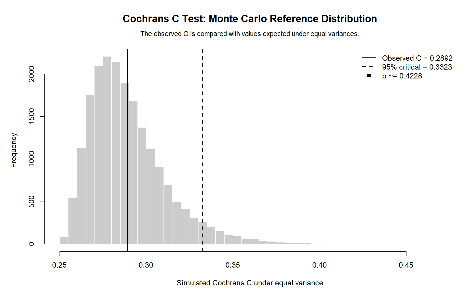
Detailed interpretation: The R Monte Carlo reference chart validates the simulation-based interpretation of the observed C statistic. It helps readers understand whether the largest variance share is unusual under an equal-variance assumption.
Decision / reporting conclusion: The R reference distribution supports the practical conclusion that the observed variance share is not strong evidence of serious variance heterogeneity.
R Chart 5: Group Size and Variance
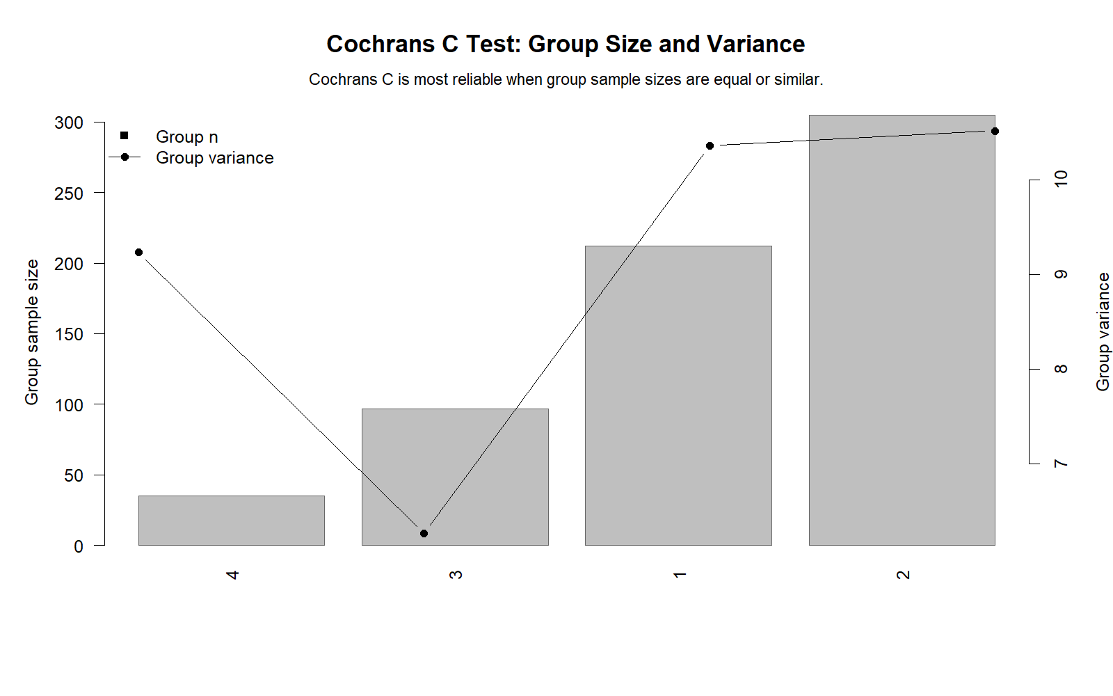
Detailed interpretation: This R chart confirms that the group sizes are unequal: group 2 is largest, and group 4 is smallest. It is important to interpret variance estimates in light of group size because small groups can have unstable variance estimates.
Decision / reporting conclusion: R confirms that the largest variance occurs in the largest group, which makes the variance comparison more stable than if the largest variance came from the smallest group.
R Chart 6: Cochran’s C Across Groupings
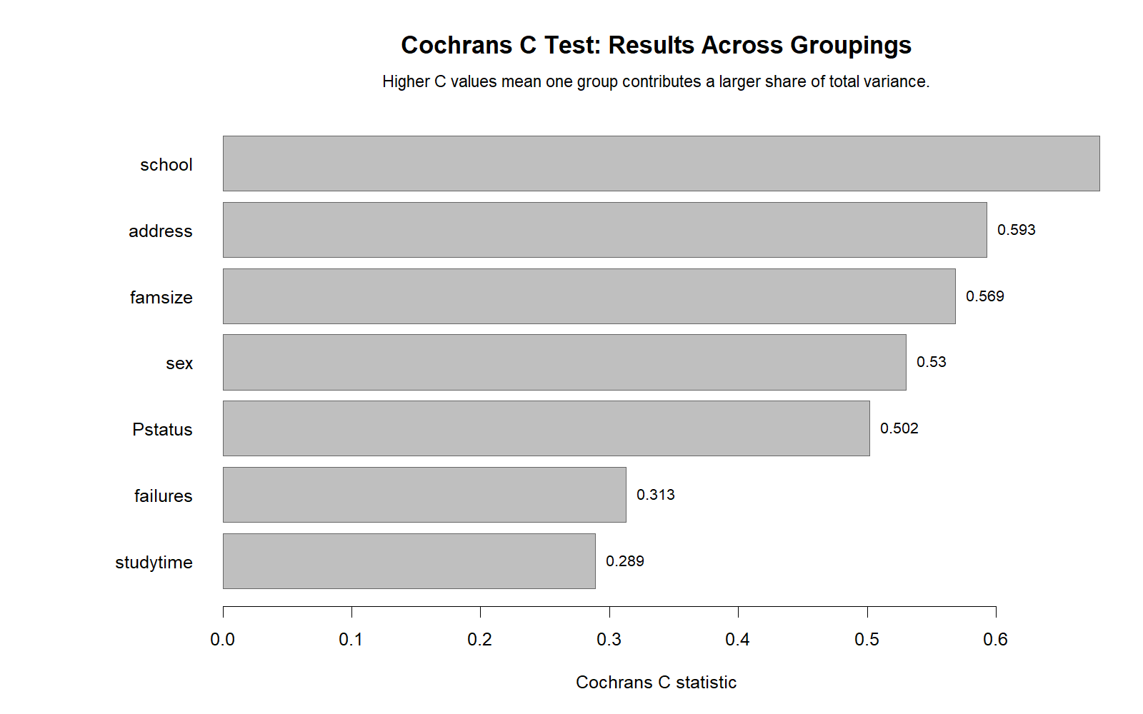
Detailed interpretation: The R grouping comparison confirms that Cochran’s C can change depending on the grouping variable. This helps analysts understand that variance homogeneity is not only about the outcome variable but also about how the sample is split into groups.
Decision / reporting conclusion: R validates the broader diagnostic use of Cochran’s C across multiple group definitions.
SPSS, Python, R and Excel Workflows for Cochran’s C Test
The Cochran’s C Test workflow is based on computing group variances, identifying the largest variance, summing all group variances, and calculating the largest variance share. The result should be interpreted with group sizes, boxplots, Levene comparison, and the purpose of the analysis.
SPSS Workflow
| Step | SPSS Menu or Syntax | Purpose |
|---|---|---|
| Open dataset | File > Open > Data | Load the SPSS-ready dataset. |
| Generate group descriptives | Analyze > Compare Means > Means | Get N, mean, standard deviation and variance by group. |
| Inspect group spread | Analyze > Descriptive Statistics > Explore | Create boxplots, histograms and Q-Q plots. |
| Calculate Cochran’s C | Syntax or aggregate calculation | Divide largest variance by total variance. |
| Compare with Levene | Analyze > Compare Means > One-Way ANOVA > Homogeneity | Use Levene as supporting homogeneity evidence. |
| Export output | OUTPUT EXPORT | Save the SPSS PDF for reporting and WordPress resources. |
Python Workflow
| Step | Python Action | Purpose |
|---|---|---|
| Read data | pandas.read_csv() | Load the dataset. |
| Group data | df.groupby("studytime") | Split G3 by studytime groups. |
| Calculate variances | groupby().var(ddof=1) | Compute sample variance in each group. |
| Calculate Cochran’s C | variances.max() / variances.sum() | Get largest variance share. |
| Create charts | matplotlib | Build boxplots, variance bars, share charts and reference distributions. |
| Report decision | APA wording | Write statistic and variance interpretation. |
R Workflow
| Step | R Action | Purpose |
|---|---|---|
| Read data | read.csv() or readr::read_csv() | Load the dataset. |
| Group data | group_by(studytime) | Prepare group-level summaries. |
| Calculate variances | summarise(var_G3 = var(G3)) | Compute group variances. |
| Calculate Cochran’s C | max(var_G3) / sum(var_G3) | Compute largest variance share. |
| Create validation charts | ggplot2 | Validate Python and SPSS results visually. |
| Write report | APA wording | Summarize statistic, group variances and decision. |
Excel Workflow
| Excel Task | Formula or Tool | Purpose |
|---|---|---|
| Separate groups | Filter or PivotTable | Place G3 values by studytime group. |
| Calculate each variance | =VAR.S(range) | Compute group sample variance. |
| Find largest variance | =MAX(variance_cells) | Identify max group variance. |
| Sum variances | =SUM(variance_cells) | Calculate total variance denominator. |
| Calculate Cochran’s C | =MAX(variance_cells)/SUM(variance_cells) | Compute largest variance share. |
| Create chart | Insert > Column Chart | Visualize group variances. |
If Cochran’s C is being used before ANOVA, the assumption workflow can also include Central Limit Theorem considerations, normality plots, the effect size of the final comparison, and confidence intervals for group means.
Code Blocks for Cochran’s C Test
SPSS Syntax for Cochran’s C Test
* Cochran's C Test in SPSS.
* Outcome: G3 final grade.
* Grouping variable: studytime.

TITLE "Cochran's C Test: G3 by studytime".

GET FILE='D:\DATA ANALYSIS\B Normality and Assumption Tests\Cochrans C Test\SPSS_Output\sav\Cochran-C-Test-data.sav'.

MEANS TABLES=G3 BY studytime
  /CELLS=COUNT MEAN STDDEV VARIANCE.

EXAMINE VARIABLES=G3 BY studytime
  /PLOT BOXPLOT HISTOGRAM NPPLOT
  /COMPARE GROUPS
  /STATISTICS DESCRIPTIVES
  /CINTERVAL 95
  /MISSING LISTWISE
  /NOTOTAL.

ONEWAY G3 BY studytime
  /STATISTICS DESCRIPTIVES HOMOGENEITY
  /MISSING ANALYSIS.

* Verified values from SPSS output.
DATASET DECLARE CochranC_Result.
DATASET ACTIVATE CochranC_Result.

INPUT PROGRAM.
NUMERIC number_of_groups total_n min_n max_n sum_variance max_variance cochran_c.
END CASE.
END FILE.
END INPUT PROGRAM.

COMPUTE number_of_groups = 4.
COMPUTE total_n = 649.
COMPUTE min_n = 35.
COMPUTE max_n = 305.
COMPUTE sum_variance = 36.36986.
COMPUTE max_variance = 10.51786.
COMPUTE cochran_c = max_variance / sum_variance.
EXECUTE.

FORMATS number_of_groups min_n max_n (F8.0)
  total_n sum_variance max_variance cochran_c (F12.5).

LIST number_of_groups total_n min_n max_n sum_variance max_variance cochran_c.

OUTPUT SAVE OUTFILE='D:\DATA ANALYSIS\B Normality and Assumption Tests\Cochrans C Test\SPSS_Output\spv\Cochran-C-Test-output.spv'.

OUTPUT EXPORT
  /CONTENTS EXPORT=VISIBLE LAYERS=PRINTSETTING MODELVIEWS=PRINTSETTING
  /PDF DOCUMENTFILE='D:\DATA ANALYSIS\B Normality and Assumption Tests\Cochrans C Test\SPSS_Output\pdf\Cochran-C-Test-SPSS-Output.pdf'.
Python Code for Cochran’s C Test
import pandas as pd
import numpy as np
import matplotlib.pyplot as plt

# Load data
df = pd.read_csv("dataset.csv")

# Keep needed variables
data = df[["G3", "studytime"]].dropna()
data["G3"] = pd.to_numeric(data["G3"], errors="coerce")
data["studytime"] = data["studytime"].astype(str)
data = data.dropna()

# Group summary
summary = data.groupby("studytime")["G3"].agg(
    N="count",
    Mean="mean",
    SD="std",
    Variance=lambda x: x.var(ddof=1)
).reset_index()

print(summary)

# Cochran's C
variances = summary["Variance"]
max_variance = variances.max()
sum_variance = variances.sum()
cochran_c = max_variance / sum_variance

print("Number of groups:", len(summary))
print("Total N:", summary["N"].sum())
print("Minimum group N:", summary["N"].min())
print("Maximum group N:", summary["N"].max())
print("Largest variance:", max_variance)
print("Sum of variances:", sum_variance)
print("Cochran's C:", cochran_c)

# Boxplot
groups = [g["G3"].values for _, g in data.groupby("studytime")]
labels = [name for name, _ in data.groupby("studytime")]

plt.figure(figsize=(10, 6))
plt.boxplot(groups, labels=labels)
plt.title("Cochran's C Test: G3 Group Spread by Studytime")
plt.xlabel("Studytime group")
plt.ylabel("G3 final grade")
plt.tight_layout()
plt.show()

# Group variance comparison
plt.figure(figsize=(10, 6))
plt.bar(summary["studytime"], summary["Variance"])
plt.title("Group Variance Comparison for Cochran's C Test")
plt.xlabel("Studytime group")
plt.ylabel("Variance of G3")
plt.tight_layout()
plt.show()

# Largest variance share
shares = summary["Variance"] / summary["Variance"].sum()
plt.figure(figsize=(10, 6))
plt.bar(summary["studytime"], shares)
plt.title("Largest Variance Share")
plt.xlabel("Studytime group")
plt.ylabel("Variance share")
plt.tight_layout()
plt.show()

# Simple Monte Carlo reference distribution
rng = np.random.default_rng(123)
n_sim = 10000
group_sizes = summary["N"].to_numpy()
pooled_sd = data["G3"].std(ddof=1)

sim_c = []
for _ in range(n_sim):
    sim_vars = []
    for n in group_sizes:
        y = rng.normal(loc=0, scale=pooled_sd, size=int(n))
        sim_vars.append(np.var(y, ddof=1))
    sim_vars = np.array(sim_vars)
    sim_c.append(sim_vars.max() / sim_vars.sum())

sim_c = np.array(sim_c)
p_upper = np.mean(sim_c >= cochran_c)

print("Monte Carlo upper-tail probability:", p_upper)
R Code for Cochran’s C Test
library(readr)
library(dplyr)
library(ggplot2)

# Load data
df <- read_csv("dataset.csv")

# Prepare data
data <- df |>
  select(G3, studytime) |>
  filter(!is.na(G3), !is.na(studytime)) |>
  mutate(studytime = as.factor(studytime))

# Group summary
summary_tbl <- data |>
  group_by(studytime) |>
  summarise(
    N = n(),
    Mean = mean(G3),
    SD = sd(G3),
    Variance = var(G3),
    .groups = "drop"
  )

print(summary_tbl)

# Cochran's C
max_variance <- max(summary_tbl$Variance)
sum_variance <- sum(summary_tbl$Variance)
cochran_c <- max_variance / sum_variance

cat("Number of groups:", nrow(summary_tbl), "\n")
cat("Total N:", sum(summary_tbl$N), "\n")
cat("Minimum group N:", min(summary_tbl$N), "\n")
cat("Maximum group N:", max(summary_tbl$N), "\n")
cat("Largest variance:", max_variance, "\n")
cat("Sum of variances:", sum_variance, "\n")
cat("Cochran's C:", cochran_c, "\n")

# Boxplot
ggplot(data, aes(x=studytime, y=G3)) +
  geom_boxplot() +
  labs(title="Cochran's C Test: G3 Group Spread by Studytime",
       x="Studytime group",
       y="G3 final grade")

# Variance comparison
ggplot(summary_tbl, aes(x=studytime, y=Variance)) +
  geom_col() +
  labs(title="Group Variance Comparison",
       x="Studytime group",
       y="Variance of G3")

# Largest variance share
summary_tbl <- summary_tbl |>
  mutate(VarianceShare = Variance / sum(Variance))

ggplot(summary_tbl, aes(x=studytime, y=VarianceShare)) +
  geom_col() +
  labs(title="Largest Variance Share",
       x="Studytime group",
       y="Variance share")

# Monte Carlo reference distribution
set.seed(123)
n_sim <- 10000
group_sizes <- summary_tbl$N
pooled_sd <- sd(data$G3)

sim_c <- replicate(n_sim, {
  sim_vars <- sapply(group_sizes, function(n) var(rnorm(n, mean=0, sd=pooled_sd)))
  max(sim_vars) / sum(sim_vars)
})

p_upper <- mean(sim_c >= cochran_c)
cat("Monte Carlo upper-tail probability:", p_upper, "\n")
Excel Formulas for Cochran’s C Test
Assume group variances are in cells B2:B5.

Studytime group 1 variance:
=VAR.S(group1_G3_range)

Studytime group 2 variance:
=VAR.S(group2_G3_range)

Studytime group 3 variance:
=VAR.S(group3_G3_range)

Studytime group 4 variance:
=VAR.S(group4_G3_range)

Largest variance:
=MAX(B2:B5)

Sum of variances:
=SUM(B2:B5)

Cochran's C statistic:
=MAX(B2:B5)/SUM(B2:B5)

Using verified values:
=10.51786/36.36986

Result:
0.28919

Interpretation:
The largest variance contributes about 28.9% of the total variance share.
APA Reporting Wording for Cochran’s C Test
When reporting Cochran’s C Test, include the outcome variable, grouping variable, number of groups, group variances, largest variance, total variance, C statistic, and a clear decision about the homogeneity of variance assumption.
APA-Style Cochran’s C Test Report
Cochran’s C Test was used to evaluate whether the largest variance in G3 final grades across studytime groups was unusually large. The group variances were 10.360, 10.518, 6.261, and 9.232. The largest variance was 10.51786, and the sum of variances was 36.36986, producing Cochran’s C = .28919. The largest variance represented approximately 28.9% of the total variance share. A supporting Levene test was non-significant, F(3, 645) = .985, p = .400, indicating no strong evidence against homogeneity of variance.
Short Report Sentence
Cochran’s C Test indicated that the largest G3 variance across studytime groups accounted for 28.9% of the total variance share, C = .28919; the supporting Levene test was non-significant, p = .400, so the variance homogeneity assumption appeared acceptable.
Student-Friendly Report Example
The largest group variance was found in studytime group 2, but it was not large enough to dominate the total variance pattern. Therefore, the spread of final grades across studytime groups appears reasonably similar for practical ANOVA reporting.
If the final analysis also reports mean differences, include the ANOVA result and a practical magnitude measure. Use effect size for practical importance and confidence intervals for uncertainty around mean estimates.
Common Mistakes in Cochran’s C Test Interpretation
| Mistake | Why It Is a Problem | Correct Practice |
|---|---|---|
| Interpreting Cochran’s C as a mean test | Cochran’s C evaluates variance spread, not mean differences. | Use ANOVA for means and Cochran’s C for largest variance share. |
| Ignoring group sizes | Small groups can produce unstable variance estimates. | Report minimum and maximum group sizes with the C statistic. |
| Reporting only the largest variance | The test depends on the largest variance relative to all variances. | Report largest variance, sum of variances and C statistic. |
| Ignoring visual spread | A statistic alone does not show how spread differs across groups. | Use boxplots and group variance charts. |
| Forgetting Levene comparison | Levene is a widely recognized homogeneity test. | Use Levene or Brown-Forsythe as supporting evidence. |
| Confusing Cochran’s C with Cochran’s Q | Cochran’s Q is for related binary outcomes, not group variances. | Use Cochran’s C for largest variance share across groups. |
Key reminder: Cochran’s C Test is a variance diagnostic. It does not replace normality checks, model diagnostics, or substantive interpretation of the final research question.
When to Use Cochran’s C Test
Use Cochran’s C Test when you want to know whether the largest group variance is unusually large compared with the total group variance. It is especially useful in group-comparison workflows, assumption checking, and educational examples where variance shares need to be explained clearly.
| Use Case | Why Cochran’s C Helps | Example from This Guide |
|---|---|---|
| Checking variance homogeneity | Identifies whether one group variance dominates. | G3 variances were compared across studytime groups. |
| Preparing for ANOVA | Variance homogeneity is an important ANOVA assumption. | Levene comparison supported homogeneity. |
| Explaining largest variance share | C is easy to interpret as a proportion. | C = .28919 means the largest variance share was about 28.9%. |
| Comparing group structures | C can be recalculated across grouping variables. | Python and R charts compare Cochran’s C across groupings. |
| Teaching variance diagnostics | The formula is simple and visually intuitive. | Largest variance divided by total variance. |
If variance homogeneity is violated, consider robust alternatives, transformations, Welch-style procedures, or model-based approaches depending on the research design. If non-normality is also present, check Q-Q plots, P-P plots, D’Agostino-Pearson test, Cramér-von Mises test, and Ryan-Joiner test. For model-form problems, see the Ramsey RESET test; for heteroscedasticity in regression, see the Goldfeld-Quandt test.
Downloads and Resources for Cochran’s C Test
The resources below include the SPSS output PDF, Python charts, and R validation charts used in this Cochran’s C Test guide.
Download SPSS Output PDF
Verified SPSS output for G3 by studytime, group variances, Cochran’s C calculation, Levene comparison, ANOVA context and normality checks.
Copy Cochran’s C Test Code
Use the SPSS, Python, R and Excel code blocks to reproduce the Cochran’s C workflow.
Python Chart 1: Group Spread Boxplots
Visual group spread comparison for G3 by studytime.
R Chart 1: Group Spread Boxplots
R validation chart for group spread interpretation.
FAQs About Cochran’s C Test
What is Cochran’s C Test?
Cochran’s C Test is a variance homogeneity test that checks whether the largest group variance is unusually large compared with the sum of all group variances.
What does Cochran’s C statistic mean?
Cochran’s C is the largest group variance divided by the sum of all group variances. It can be interpreted as the largest variance share.
What was the Cochran’s C result in this guide?
The verified result was C = .28919 for G3 across four studytime groups. The largest variance was 10.51786 and the sum of variances was 36.36986.
Which group had the largest variance?
Studytime group 2 had the largest variance, 10.518, and it also had the largest group size, N = 305.
Does Cochran’s C Test compare means?
No. Cochran’s C Test compares variance spread, not group means. ANOVA compares means, while Cochran’s C helps check whether one group variance is unusually large.
How is Cochran’s C related to Levene’s test?
Both are variance homogeneity checks. Cochran’s C focuses on the largest variance share, while Levene’s test evaluates variance equality more generally. In this guide, Levene’s test was non-significant, p = .400.
Can Cochran’s C Test be calculated in Excel?
Yes. Calculate each group variance with VAR.S, find the largest variance with MAX, sum all variances with SUM, and divide MAX by SUM.
What should I do if Cochran’s C suggests unequal variances?
Check boxplots, group sizes, Levene or Brown-Forsythe tests, and consider robust methods, Welch-style analysis, transformations, or a model that handles unequal variances.
Final Conclusion
The Cochran’s C Test is a simple and useful variance diagnostic because it asks whether the largest group variance dominates the total variance pattern. In this Salar Cafe example, G3 final grades were compared across four studytime groups. The largest variance was 10.51786, the sum of variances was 36.36986, and the verified Cochran’s C statistic was .28919.
The Python and R charts support the same interpretation. The group spread boxplots show some differences in spread, the largest variance share chart explains the C statistic, the variance comparison chart identifies studytime group 2 as the largest variance group, and the Monte Carlo reference charts help interpret whether the observed C statistic is unusual. The supporting SPSS Levene test is non-significant, p = .400, so the homogeneity of variance assumption appears acceptable.
The correct reporting conclusion is not simply “all groups are identical.” The correct conclusion is that the largest variance is identifiable but not extreme enough to create a serious variance homogeneity concern. For a professional report, combine Cochran’s C with descriptive statistics, boxplots, Levene’s test, normality checks, and the final ANOVA or model result.

