
Panel Regression: Formula, Interpretation, Fixed Effects, Python, R, SPSS and Excel Guide
Panel Regression analyses repeated measurements from the same units over time. It can separate persistent differences between students from changes occurring within each student across G1, G2, and G3.
3 time periods
1,947 panel rows
Pooled, fixed-effects, and first-difference models
Model Overview
Panel Regression is a family of regression methods for data that follow the same people, organisations, regions, firms, countries, or other units across multiple time periods. The defining feature is repeated observation: each unit contributes more than one row, so the records are connected rather than independent. Panel Regression uses that structure to study both differences between units and movement within the same unit over time.
The method is used when a research question includes time and repeated measurement. Typical examples include annual company performance, patient outcomes across clinical visits, household income across survey waves, regional economic indicators across years, or student achievement measured at several assessment points. A conventional Multiple Linear Regression model can analyse a single cross-section, but it cannot fully distinguish whether a relationship reflects stable differences between units or genuine change within units.
Panel Regression is valuable because many unobserved characteristics remain stable over the study period. Motivation, background ability, organisational culture, geography, family environment, and other persistent influences may affect the outcome even when they are not directly measured. Entity fixed effects remove all time-invariant unit characteristics, observed or unobserved, allowing the model to focus on within-unit change. Time fixed effects control common shocks or period differences affecting all units.
Several specifications fall under the Panel Regression label. Pooled OLS stacks all observations and estimates one common equation. Time fixed effects adds period indicators. Entity fixed effects controls each unit’s stable average level. First difference models changes between adjacent observations. Random effects, Mixed Effects Regression, Hierarchical Linear Model, and Generalized Estimating Equations offer related approaches when the assumptions and research goals differ.
Choosing among these models depends on the question, not only on which model has the largest R-squared. Pooled OLS is often strongest for describing between-unit differences. Entity fixed effects is preferable when the target is change within the same unit and unobserved stable characteristics may be correlated with predictors. First difference is useful when change itself is the outcome. A random-effects approach can estimate both time-varying and time-invariant predictors efficiently when its independence assumption is defensible.
Panel Regression coefficients retain the familiar regression interpretation, but the source of variation matters. A pooled coefficient may combine between-student and within-student information. An entity fixed-effects coefficient uses only within-student movement. These estimates can differ because students who generally have higher values are not necessarily the same students who improve when a predictor changes.
The principal assumptions include a correctly specified functional form, no perfect multicollinearity, appropriate treatment of dependence within units, and an error structure compatible with the reported standard errors. Fixed-effects models also require predictors to vary over time; a time-invariant variable cannot be estimated separately after entity demeaning. Serial correlation, heteroskedasticity, and cross-sectional dependence may require clustered or robust standard errors.
In this worked example, the original dataset contains 649 students and three repeated grade columns: G1, G2, and G3. These columns are reshaped into a long panel containing 1,947 rows, with student_id identifying the unit, panel_time identifying the wave, and panel_grade serving as the repeated outcome. The article compares pooled OLS, time fixed effects, entity fixed effects, and first-difference models.
The results reveal a modest upward time trend but much larger differences between students. Pooled OLS has the highest reported adjusted R-squared at 0.2724, whereas entity fixed effects explains 5.07% of within-student variation and first difference explains only 0.28%. The contrast is central to the analysis: stable student-level differences dominate the total variation, while average movement over three periods is comparatively small.
Quick Answer
Main pattern
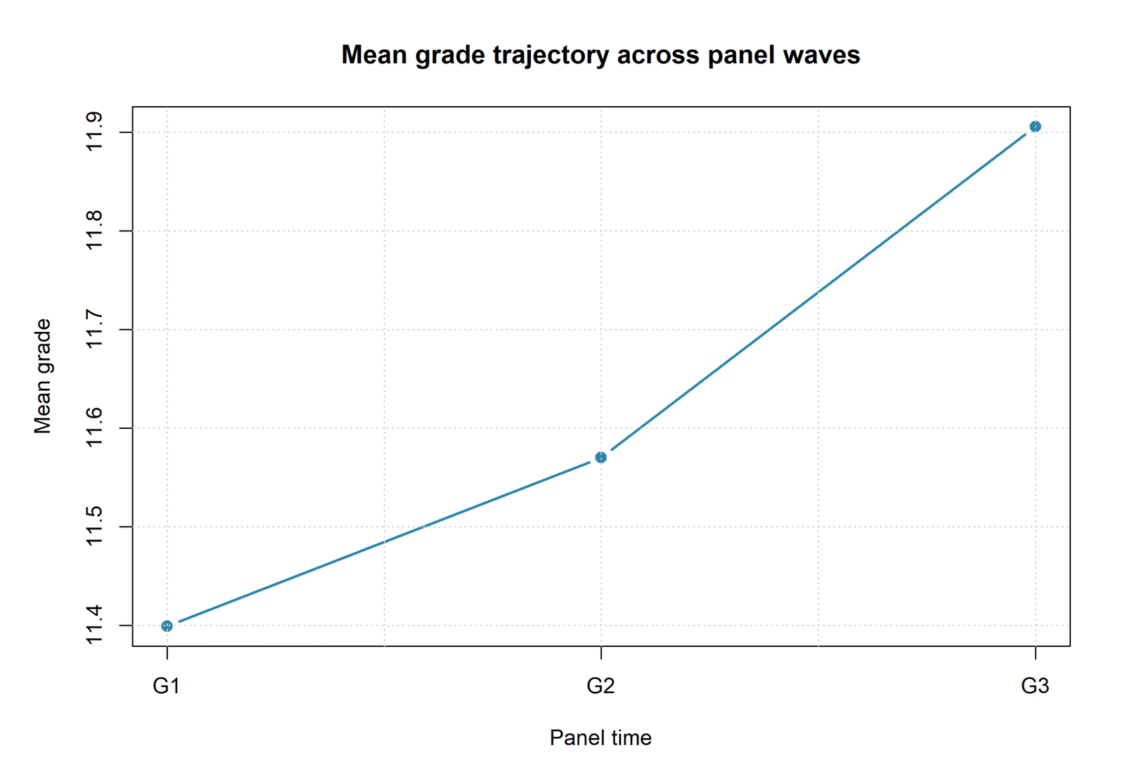
- Mean grade rises from 11.399 at G1 to 11.906 at G3.
- The entity fixed-effects time coefficient is 0.2535 per wave.
- Most variation reflects persistent differences between students.
Model comparison
- Pooled adjusted R²: 0.2724
- Time fixed effects: 0.2722
- Entity fixed effects: 0.0507
- First difference: 0.0028
Table of Contents
- What Panel Regression is
- When and why it is used
- Pooled, fixed-effects, and first-difference models
- Formulas and coefficient interpretation
- Panel construction and variables
- Results at a glance
- Eight panel chart explanations
- R chart interpretations
- Coefficients and model fit
- Within-student and between-student findings
- Diagnostics and model choice
- Python, R, SPSS, and Excel workflows
- Code
- Advanced interpretation
- APA-style reporting
- Publication checklist
- Downloads
- Related guides
- Frequently asked questions
What Is Panel Regression?
Panel Regression models repeated outcomes from the same units over time. The same student, patient, company, household, or country appears in several periods, creating a two-dimensional dataset with a unit dimension and a time dimension.
The method differs from a purely cross-sectional regression because observations belonging to the same unit are connected. It also differs from a single time-series model because the dataset contains many units rather than one sequence. Panel Regression combines both structures and can identify patterns that would be hidden in either a single cross-section or a single aggregate trend.
The principal analytical distinction is between between-unit variation and within-unit variation. Between-unit variation asks why some students generally achieve higher grades than others. Within-unit variation asks whether the same student’s grade changes as time or another time-varying predictor changes. These questions can produce different coefficients and should not be treated as interchangeable.
When and Why Panel Regression Is Used
Panel Regression is used when repeated observations are central to the research design. It can improve control for omitted stable characteristics, increase the number of observations available for estimation, and distinguish long-term differences from short-term change.
A student panel illustrates the benefit. A pooled model may find that studytime is associated with higher grades because students who generally study more also generally perform better. A within-student model asks a different question: does a particular student’s grade rise during periods when that student’s studytime increases? Only the second interpretation isolates within-student change.
Related methods include Fixed Effects Regression, Mixed Effects Regression, Hierarchical Linear Model, Generalized Estimating Equations, and Generalized Least Squares Regression. The correct choice depends on whether the target is subject-specific change, population-average association, random variation, or efficient modelling of a known covariance structure.
Pooled, Time Fixed-Effects, Entity Fixed-Effects, and First-Difference Models
| Specification | Source of information | Main question | Main limitation |
|---|---|---|---|
| Pooled OLS | Between and within variation combined | Which observed characteristics are associated with grade levels across all rows? | Treats stable unobserved student differences as part of the error unless addressed separately |
| Time fixed effects | Between and within variation plus wave indicators | Are G2 and G3 systematically different from G1 after adjustment? | Does not remove stable student-level confounding |
| Entity fixed effects | Within-student variation only | How does the same student’s grade change as time advances? | Cannot estimate time-invariant predictors separately |
| First difference | Change between adjacent waves | Does the size of grade change differ between transitions? | Differencing removes stable information and can magnify measurement noise |
No single specification is universally superior. Pooled OLS best describes total observed variation in this example, while entity fixed effects provides the most direct estimate of average within-student movement. First difference focuses only on adjacent-wave changes and therefore has a different denominator and interpretation. This Panel Regression distinction is essential when comparing specifications.
Panel Regression Formulas and Interpretation
In the pooled model, the coefficient for time_index is the average grade difference associated with moving forward one wave after the observed student characteristics are held constant. Because the model combines within- and between-student information, it is not purely a change estimate.
In the entity fixed-effects model, every variable is expressed as a deviation from that student’s mean. The coefficient therefore represents average within-student movement and is protected against confounding from all stable student characteristics, whether measured or not.
The first-difference model subtracts one wave from the previous wave. Its transition coefficient measures whether the average change from G2 to G3 differs from the average change from G1 to G2.
Panel Construction and Variables
| Variable | Role | Definition | Used in |
|---|---|---|---|
| student_id | Panel unit | Original student row number | Entity identification and demeaning |
| panel_time | Time label | G1, G2, or G3 | Time fixed effects and charts |
| time_index | Numeric time | 1 for G1, 2 for G2, 3 for G3 | Pooled and entity fixed-effects trend |
| panel_grade | Repeated outcome | Grade observed at the corresponding wave | All level models |
| grade_change | Differenced outcome | Current grade minus previous grade | First-difference model |
| studytime | Predictor | Weekly study-time category | Pooled and time fixed effects |
| failures | Predictor | Prior class failures | Pooled and time fixed effects |
| absences | Predictor | School absences | Pooled and time fixed effects |
| age, Medu, Fedu | Predictors | Age and parental education | Pooled and time fixed effects |
| school, sex, address | Categorical predictors | Student background categories | Pooled and time fixed effects |
The panel is balanced: all 649 students contribute all three waves, producing exactly 1,947 level observations and 1,298 adjacent-wave differences.
Results at a Glance
RMSE 2.5313
RMSE 2.5310
RMSE 0.8907
RMSE 1.3814
p < .001
p = .0319
Eight Panel Regression Chart Explanations
Each figure is organised around the visible pattern, the values that define it, the statistical interpretation, and its relevance to the reader.
Chart 1: Mean Grade Across G1, G2, and G3
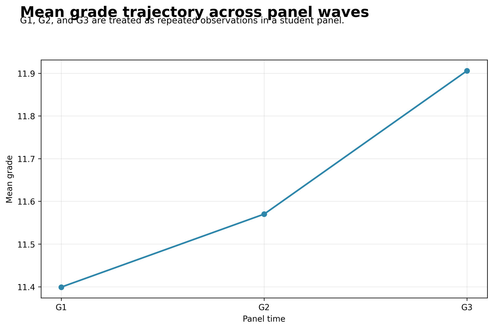
The sample mean increases at each wave. The rise from G1 to G2 is modest, followed by a larger increase from G2 to G3.
G1 mean = 11.399, G2 mean = 11.570, and G3 mean = 11.906. The average increase is about 0.171 points from G1 to G2 and 0.336 points from G2 to G3.
The cohort improves slightly over time, but the movement is small compared with the differences between students. The upward average does not mean every student improved; individual trajectories include increases, declines, and stable grades.
The time trend is statistically detectable, yet it explains only a limited share of the total grade variation. Panel Regression is valuable here because it separates this common time movement from persistent differences between students.
Chart 2: Sample Student Grade Trajectories
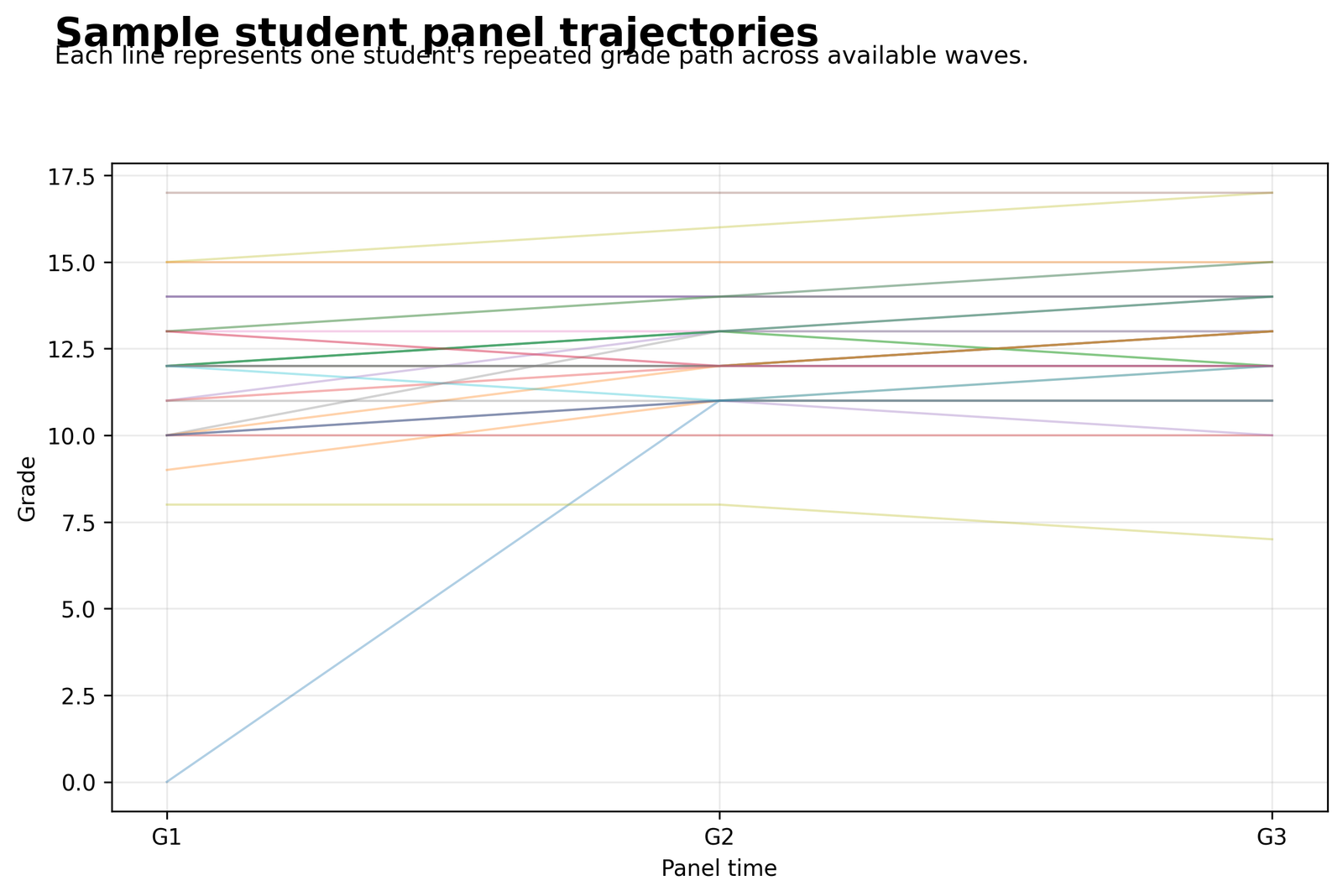
Some students remain almost unchanged, others improve gradually, a few decline, and one sampled trajectory rises sharply from a zero G1 score to 11 at G2 and G3.
Examples from the workbook include student 1: 0 → 11 → 11; student 4: 14 → 14 → 14; student 8: 10 → 13 → 13; and student 9: 15 → 16 → 17.
The mean trajectory hides substantial individual diversity. A single population average cannot represent students whose paths differ in direction, size, and stability. Stable high performers, gradual improvers, declining students, and unusual jumps coexist in the same panel.
Repeated observations should not be treated as independent records. The lines belong to the same students, so a panel model must account for the connection between each student’s three measurements.
Chart 3: Distribution of the Stacked Panel Outcome
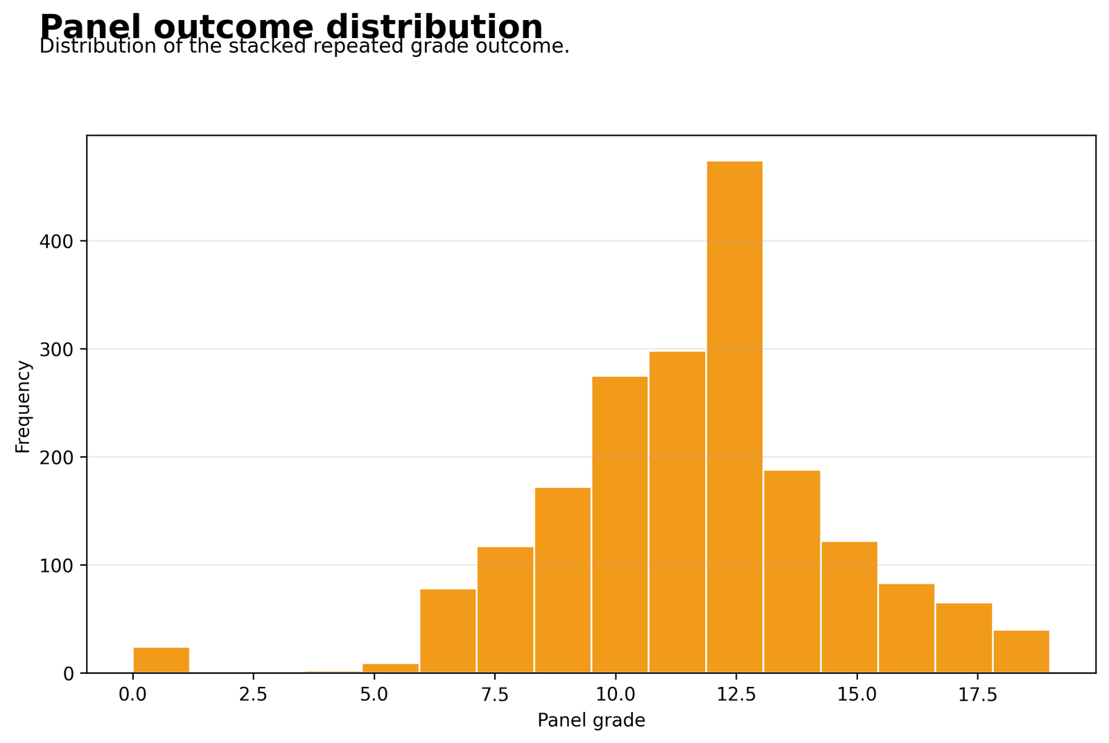
Most grades fall between about 9 and 15, with the highest concentration around 12–13. A small group of zero grades creates a separated lower tail.
The long-format panel contains 1,947 observations: 649 students measured at three waves. Scores range from 0 to 19, and the three wave means range from 11.399 to 11.906.
Stacking G1, G2, and G3 creates a dense middle distribution but also preserves unusual low outcomes. The zero-grade cases are substantively different from the central mass and contribute some of the largest pooled-model errors.
The outcome distribution informs residual interpretation and model choice. See Histogram Interpretation, Frequency Distribution, and Descriptive Statistics for the underlying descriptive concepts.
Chart 4: Observed Versus Fitted Values from Pooled OLS
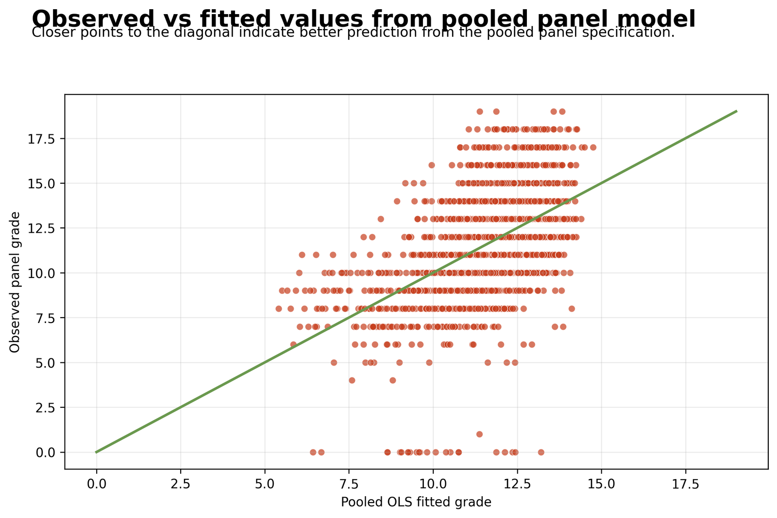
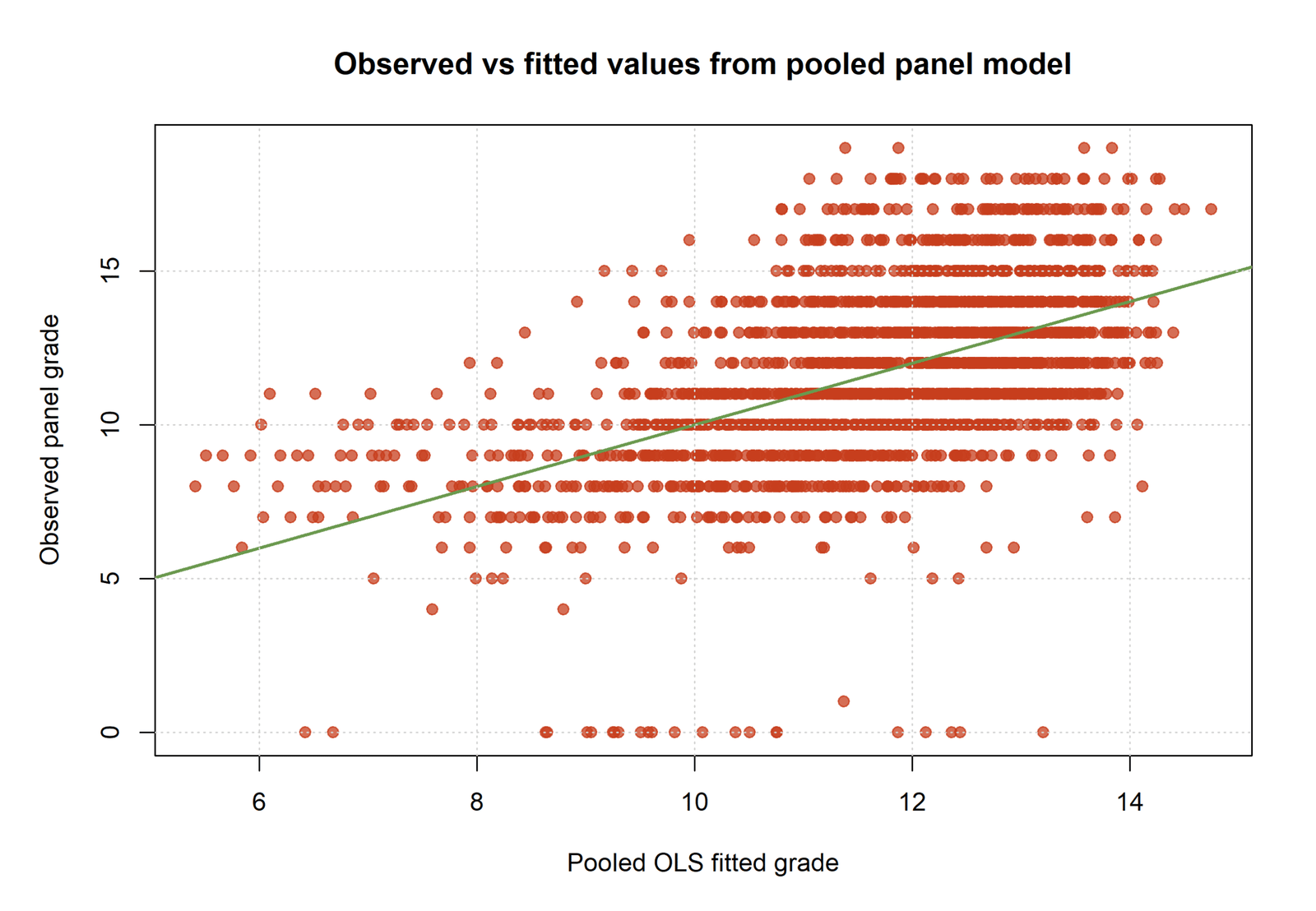
Fitted values are concentrated mainly between about 6 and 14, while observed grades extend from 0 to 19. Points follow the diagonal in broad terms but remain widely dispersed around it.
The pooled model has R² = 0.2761, adjusted R² = 0.2724, RMSE = 2.5313, and MAE = 1.9020 across 1,947 observations.
The pooled predictors explain meaningful differences in average grade levels, but they do not capture most student-specific variation. Low observed grades are often overpredicted, while some high grades are underpredicted because one common equation is applied to all students.
Pooled OLS is useful for describing between-student patterns, but it should not be mistaken for a strong individual prediction model. Its fit is the highest adjusted R² among the reported specifications because stable student characteristics explain more variation than short-term within-student movement.
Chart 5: Entity Fixed-Effects Residuals
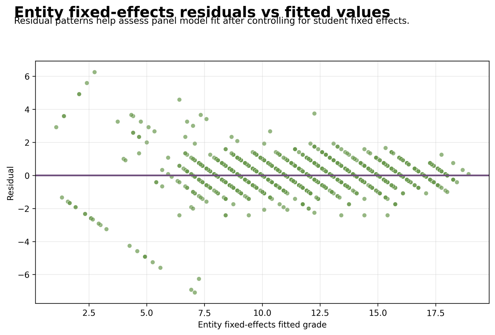
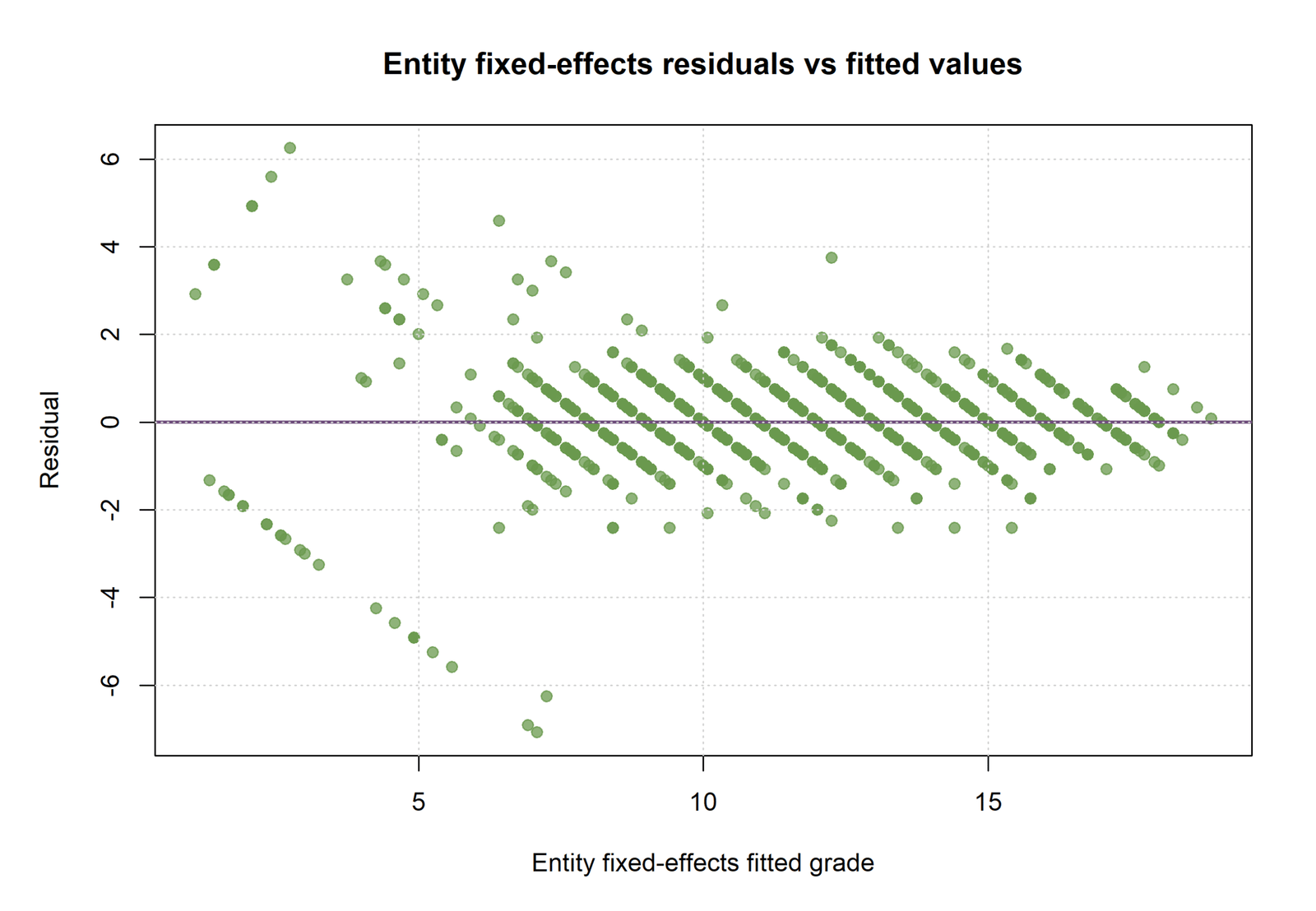
Most residuals cluster between roughly −2 and +2, with diagonal bands caused by integer-valued grades. A smaller number of cases extend beyond ±4.
The entity fixed-effects model has R² = 0.0512, adjusted R² = 0.0507, RMSE = 0.8907, and MAE = 0.5860. The within-time coefficient is 0.2535, 95% CI [0.2050, 0.3020], p < .001.
Once each student’s stable grade level is removed, the remaining changes are much smaller than the raw between-student differences. The residual spread is tight for most observations, although a few abrupt grade changes remain difficult to explain with time alone.
The lower R² does not mean the fixed-effects model is useless. It answers a narrower question: how much does a student’s grade change as time advances, after all stable student characteristics have been controlled automatically?
Chart 6: Adjusted R-Squared Across Panel Specifications
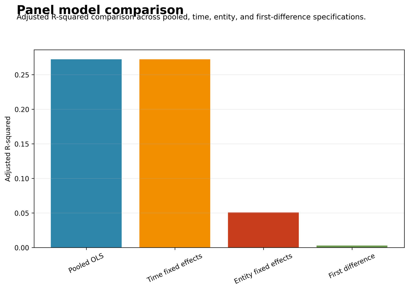
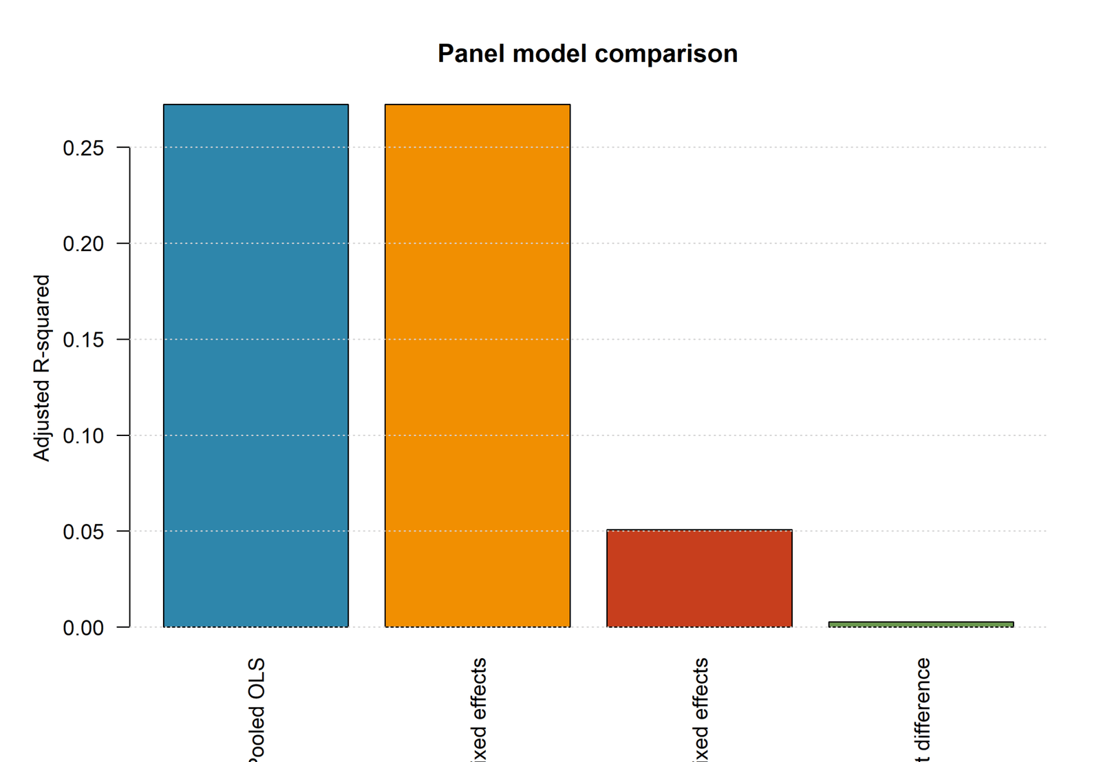
Pooled OLS and time fixed effects are nearly tied at about 0.27. Entity fixed effects falls to about 0.05, while first difference is close to zero.
Pooled OLS = 0.2724; time fixed effects = 0.2722; entity fixed effects = 0.0507; first difference = 0.0028.
Most explainable variation comes from differences between students rather than changes within the same student across three waves. Adding separate wave indicators changes pooled fit almost not at all, and differencing removes nearly all stable cross-student information.
Model fit must be matched to the question. Adjusted R-Squared is useful within comparable specifications, but pooled and within models estimate different sources of variation and should not be judged by fit alone.
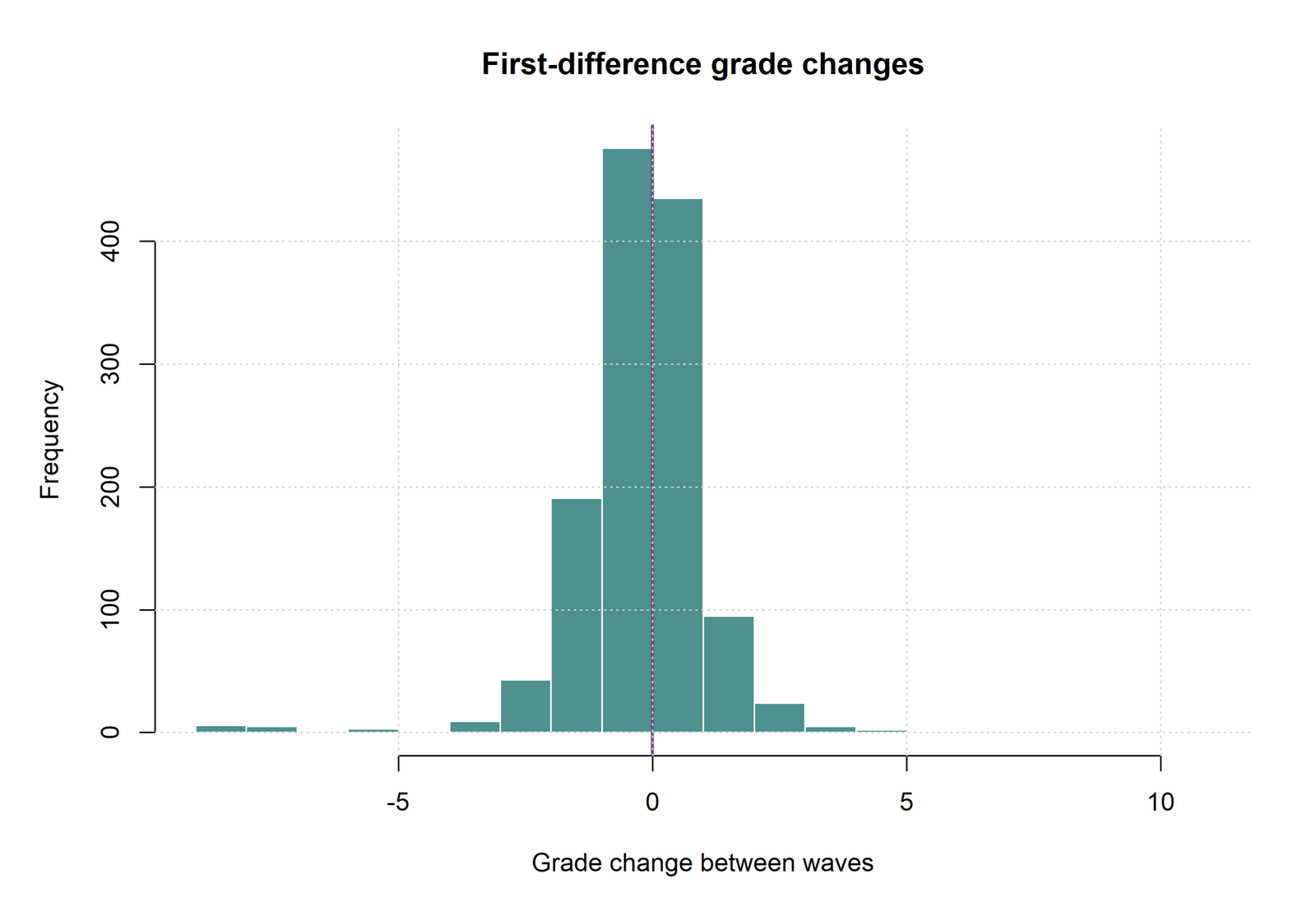
Chart 7: Distribution of First-Difference Grade Changes
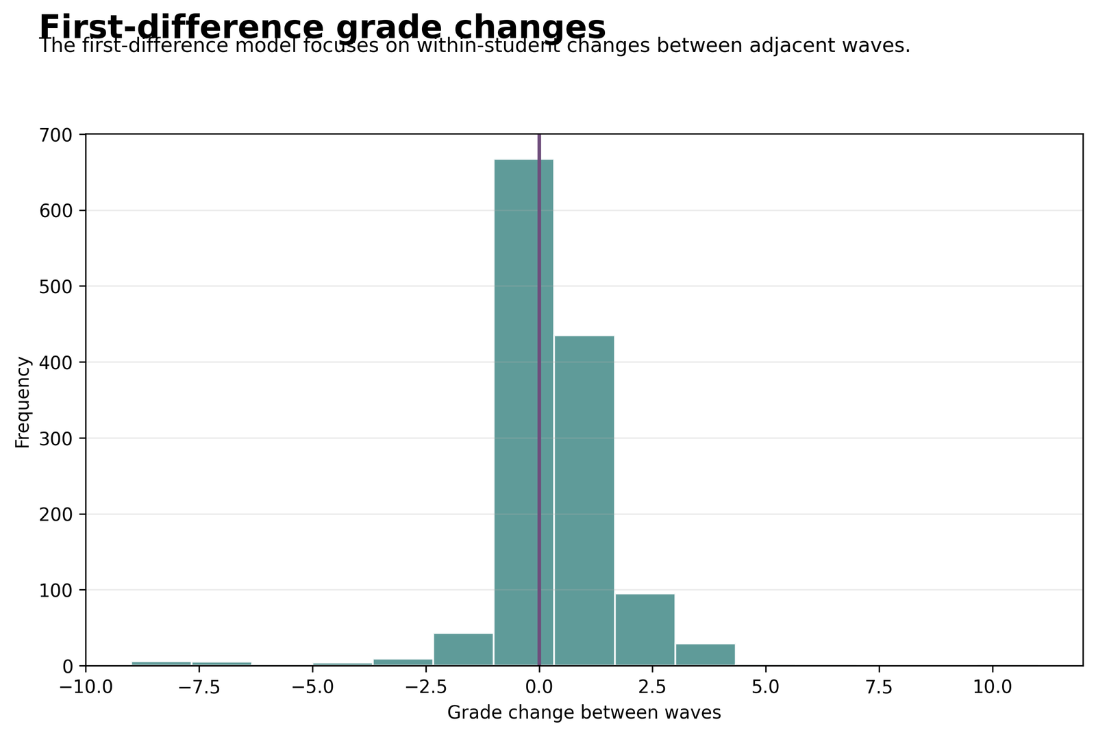
The distribution is concentrated around zero and +1. Most changes lie between approximately −1 and +2, while thin tails extend to large negative and positive changes.
There are 1,298 adjacent-wave changes. Mean change is about +0.171 for G1→G2 and +0.336 for G2→G3. The transition coefficient is 0.1649, 95% CI [0.0143, 0.3154], p = .0319.
Most students change little between neighboring periods. The later transition has a slightly larger average increase, but transition timing explains only a tiny fraction of the variation because students’ individual changes differ widely.
The statistically significant transition coefficient should be interpreted alongside adjusted R² = 0.0028. The timing difference is real on average but offers almost no power for predicting which students will improve or decline.
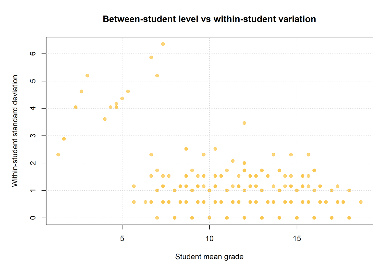
Chart 8: Student Mean Grade Versus Within-Student Variation
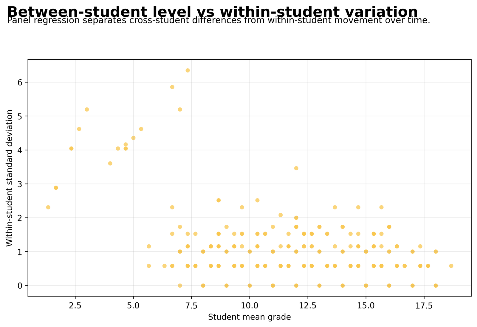
Most students have mean grades between about 8 and 18 with within-student standard deviations below 2. Lower-mean students include several unusually variable trajectories.
Workbook examples include student 1 with mean 7.333 and within-student SD 6.351; student 4 with mean 14.000 and SD 0; and student 9 with mean 16.000 and SD 1.000.
A student’s average achievement and the stability of that achievement are not the same. Two students can have similar means but very different movement across G1, G2, and G3. The largest variation is concentrated in a small set of unusual trajectories rather than across the entire cohort.
This separation is the core reason to use Panel Regression. Between-student level differences and within-student change answer different questions and should be modelled and reported separately.
R Panel Regression Charts and Interpretations
The R workflow uses the same long-format panel structure and supports pooled, fixed-effects, and first-difference analysis with the same unit and time definitions.
Mean Grade Across G1, G2, and G3
The cohort improves slightly over time, but the movement is small compared with the differences between students. The upward average does not mean every student improved; individual trajectories include increases, declines, and stable grades.
Sample Student Grade Trajectories
The mean trajectory hides substantial individual diversity. A single population average cannot represent students whose paths differ in direction, size, and stability. Stable high performers, gradual improvers, declining students, and unusual jumps coexist in the same panel.
Distribution of the Stacked Panel Outcome
Stacking G1, G2, and G3 creates a dense middle distribution but also preserves unusual low outcomes. The zero-grade cases are substantively different from the central mass and contribute some of the largest pooled-model errors.
Observed Versus Fitted Values from Pooled OLS
The pooled predictors explain meaningful differences in average grade levels, but they do not capture most student-specific variation. Low observed grades are often overpredicted, while some high grades are underpredicted because one common equation is applied to all students.
Entity Fixed-Effects Residuals
Once each student’s stable grade level is removed, the remaining changes are much smaller than the raw between-student differences. The residual spread is tight for most observations, although a few abrupt grade changes remain difficult to explain with time alone.
Adjusted R-Squared Across Panel Specifications
Most explainable variation comes from differences between students rather than changes within the same student across three waves. Adding separate wave indicators changes pooled fit almost not at all, and differencing removes nearly all stable cross-student information.
Distribution of First-Difference Grade Changes
Most students change little between neighboring periods. The later transition has a slightly larger average increase, but transition timing explains only a tiny fraction of the variation because students’ individual changes differ widely.
Student Mean Grade Versus Within-Student Variation
A student’s average achievement and the stability of that achievement are not the same. Two students can have similar means but very different movement across G1, G2, and G3. The largest variation is concentrated in a small set of unusual trajectories rather than across the entire cohort.
Panel Regression Coefficients and Model Fit
Pooled OLS coefficients
| Term | B | SE | p | 95% CI | Meaning |
|---|---|---|---|---|---|
| time_index | 0.2535 | 0.0705 | .0003 | 0.1153 to 0.3917 | Average grade rises about 0.253 points per wave after adjustment |
| studytime | 0.4640 | 0.0733 | <.001 | 0.3203 to 0.6077 | Higher studytime is associated with a higher overall grade level |
| failures | −1.5047 | 0.1056 | <.001 | −1.7118 to −1.2977 | Each additional prior failure is associated with about 1.50 fewer grade points |
| absences | −0.0671 | 0.0130 | <.001 | −0.0925 to −0.0417 | More absences are associated with a small reduction in grade level |
| age | 0.0451 | 0.0507 | .3738 | −0.0543 to 0.1445 | No reliable independent association |
| Medu | 0.2732 | 0.0684 | .0001 | 0.1391 to 0.4073 | Higher maternal education is associated with higher grades |
| Fedu | 0.1576 | 0.0692 | .0228 | 0.0220 to 0.2933 | Higher paternal education has a smaller positive association |
| school MS | −1.2579 | 0.1361 | <.001 | −1.5248 to −0.9910 | MS students have lower average grades than GP students after adjustment |
| male | −0.5800 | 0.1218 | <.001 | −0.8188 to −0.3413 | Male students have lower pooled average grades after adjustment |
| urban address | 0.2806 | 0.1347 | .0374 | 0.0164 to 0.5448 | Urban address has a small positive pooled association |
Within-student and first-difference coefficients
| Model | Term | B | SE | p | 95% CI |
|---|---|---|---|---|---|
| Entity fixed effects | within_time_index | 0.2535 | 0.0247 | <.001 | 0.2050 to 0.3020 |
| First difference | Intercept | −0.1587 | 0.1957 | .4174 | −0.5425 to 0.2251 |
| First difference | transition_time | 0.1649 | 0.0767 | .0319 | 0.0143 to 0.3154 |
The pooled coefficients describe adjusted differences in overall grade levels across students and waves. The entity fixed-effects coefficient has a narrower interpretation: within the same student, moving forward one wave is associated with an average increase of about 0.253 points. Panel Regression coefficients must always be matched to their source of variation.
Within-Student Change and Between-Student Differences
Between-student findings
- Prior failures show the largest negative pooled association.
- Studytime and parental education are positively associated with grade level.
- School, sex, and address distinguish average levels between groups.
Within-student findings
- Average grade rises about 0.253 points per wave.
- Time explains about 5.1% of demeaned grade variation.
- Most individual wave-to-wave changes remain small.
The pooled model’s adjusted R-squared of 0.2724 is largely driven by persistent differences between students. Once each student’s mean is removed, the time trend explains 0.0507 of the remaining within-student variation. This does not contradict the pooled result; it shows that the models answer different questions.
The first-difference model goes further by removing every stable level and modelling only adjacent-wave change. Its adjusted R-squared of 0.0028 indicates that knowing whether a change occurred during the first or second transition adds almost no information about the size of an individual student’s change.
Diagnostics, Standard Errors, and Model Choice
Diagnostic priorities
- Dependence within students
- Heteroskedasticity
- Serial correlation
- Influential trajectories
- Functional form and omitted time-varying predictors
Specification priorities
- Match the model to a within or between question
- Use clustered standard errors when appropriate
- Do not compare unlike R-squared values mechanically
- Justify fixed or random effects
Repeated rows from the same student are correlated. Conventional pooled OLS standard errors may therefore be too optimistic unless clustering or another appropriate covariance estimator is used. Residual checks should consider student-level clustering rather than treating all 1,947 rows as unrelated. Panel Regression inference should reflect dependence within units.
Useful supporting guides include Breusch-Pagan Test, White Test, Durbin-Watson Test, Studentized Residuals, Cook’s Distance, and Influence Diagnostics.
The fixed-effects decision should be based on whether stable unit characteristics may be correlated with the predictors. A random-effects model can be more efficient, but its independence assumption is stronger. The Hausman test is commonly used as one piece of evidence, although substantive knowledge remains essential.
Python, R, SPSS, and Excel Workflows
Python
Reshape G1, G2, and G3 into long format, fit pooled and time-indicator models, demean by student for entity fixed effects, and calculate adjacent-wave differences.
R
Use base lm() for pooled models and packages such as plm or fixest for within estimators, clustered inference, and fixed-effects diagnostics.
SPSS
Restructure repeated grade variables into cases, use MIXED for correlated repeated outcomes, or use regression with student indicators for a smaller fixed-effects application.
Excel
The worked workbook includes model-fit tables, coefficients, sample long-format data, predictions, student summaries, and live formulas demonstrating time-only predictions and residual calculations.
Code: Expand the Software You Need
Python Panel Regression code
import pandas as pd
import statsmodels.formula.api as smf

wide = pd.read_csv("dataset.csv")
wide["student_id"] = range(1, len(wide) + 1)

panel = wide.melt(
    id_vars=["student_id", "studytime", "failures", "absences",
             "age", "Medu", "Fedu", "school", "sex", "address"],
    value_vars=["G1", "G2", "G3"],
    var_name="panel_time",
    value_name="panel_grade"
)
panel["time_index"] = panel["panel_time"].map({"G1": 1, "G2": 2, "G3": 3})

pooled = smf.ols(
    "panel_grade ~ time_index + studytime + failures + absences + "
    "age + Medu + Fedu + C(school) + C(sex) + C(address)",
    data=panel
).fit()

panel["within_panel_grade"] = (
    panel["panel_grade"] - panel.groupby("student_id")["panel_grade"].transform("mean")
)
panel["within_time_index"] = (
    panel["time_index"] - panel.groupby("student_id")["time_index"].transform("mean")
)
entity_fe = smf.ols(
    "within_panel_grade ~ within_time_index - 1",
    data=panel
).fit()
R Panel Regression code
library(tidyr)
library(dplyr)
library(plm)

wide <- read.csv("dataset.csv") |>
  mutate(student_id = row_number())

panel <- wide |>
  pivot_longer(
    cols = c(G1, G2, G3),
    names_to = "panel_time",
    values_to = "panel_grade"
  ) |>
  mutate(time_index = recode(panel_time, G1 = 1, G2 = 2, G3 = 3))

pdata <- pdata.frame(panel, index = c("student_id", "time_index"))

pooled <- plm(
  panel_grade ~ time_index + studytime + failures + absences +
    age + Medu + Fedu + school + sex + address,
  data = pdata,
  model = "pooling"
)

entity_fe <- plm(
  panel_grade ~ time_index,
  data = pdata,
  model = "within",
  effect = "individual"
)
SPSS repeated-data workflow
VARSTOCASES
 /MAKE panel_grade FROM G1 G2 G3
 /INDEX=time_index(3)
 /KEEP=studytime failures absences age Medu Fedu school sex address
 /NULL=KEEP.

COMPUTE student_id = $CASENUM.
EXECUTE.

MIXED panel_grade WITH time_index studytime failures absences age Medu Fedu
 BY school sex address
 /FIXED=INTERCEPT time_index studytime failures absences age Medu Fedu
        school sex address | SSTYPE(3)
 /REPEATED=time_index | SUBJECT(student_id) COVTYPE(UN)
 /PRINT=SOLUTION TESTCOV.
Excel panel formulas
Long-format predicted value:
=Intercept + Time_Coefficient * Time_Index + Other_Predictor_Terms

Residual:
=Observed_Grade - Predicted_Grade

Squared residual:
=Residual^2

Absolute residual:
=ABS(Residual)

Student mean:
=AVERAGEIFS(Panel_Grade_Range, Student_ID_Range, Student_ID)

Within-student deviation:
=Panel_Grade - Student_Mean

First difference:
=Current_Grade - Previous_Grade
Advanced Panel Regression Interpretation
Balanced and unbalanced panels
A balanced panel contains every unit in every period. This dataset is balanced because all 649 students contribute G1, G2, and G3. Unbalanced panels can still be analysed, but missingness and attrition require closer attention. In Panel Regression, this distinction determines which observations contribute to the estimate.
Between and within estimators
The between estimator uses unit means, while the within estimator removes those means and relies only on deviations over time. Panel Regression can reveal that a predictor’s between-unit association differs from its within-unit effect.
Entity fixed effects
Fixed Effects Regression controls all stable unit characteristics through demeaning or unit indicators. It is especially useful when unobserved stable characteristics are likely to correlate with the predictors. This Panel Regression specification is strongest when the research question concerns the same unit over time.
Time fixed effects
Time indicators absorb common changes affecting every unit in a period. In this example, G3 is about 0.507 points above G1 after adjustment, while G2 is not significantly different from G1 in the categorical time specification. Within Panel Regression, the selected effects structure changes both interpretation and identification.
Two-way fixed effects
A two-way model includes both entity and time fixed effects. It controls stable unit differences and common period shocks simultaneously, but meaningful estimation still requires time-varying predictors. A two-way Panel Regression model applies this control to units and periods simultaneously.
Random effects
Random effects model unit-specific variation probabilistically and retain time-invariant predictors. They are efficient when unit effects are uncorrelated with the explanatory variables, an assumption that must be justified. Random-effects Panel Regression retains time-invariant predictors under a stronger independence assumption.
Hausman test
The Hausman test compares fixed- and random-effects estimates. A significant result is commonly interpreted as evidence against the random-effects independence assumption, although the test should not replace substantive reasoning. The Hausman comparison is commonly used when choosing a Panel Regression effects structure.
Clustered standard errors
Errors are often correlated within units. Student-clustered standard errors allow arbitrary dependence within each student’s observations while treating clusters as independent from one another. Clustered inference is often necessary because Panel Regression observations within a unit are connected.
Serial correlation
Errors may remain correlated across adjacent waves. The Durbin-Watson Test is a basic introduction, while panel-specific tests such as the Wooldridge test are more directly suited to repeated-unit data. Serial dependence can affect Panel Regression standard errors even when coefficients remain unbiased.
Heteroskedasticity
Error variance may differ between students or across fitted values. Review Breusch-Pagan Test and White Test, then use robust or clustered inference where appropriate. Heteroskedasticity should be addressed explicitly in Panel Regression inference.
Cross-sectional dependence
Units can be affected by common shocks not fully captured by time effects. Cross-sectional dependence is especially important in firm, regional, and country panels. Cross-sectional dependence matters when Panel Regression units share common shocks.
Time-invariant predictors
Entity fixed effects remove variables that never change within a unit. School, sex, and address cannot be estimated separately in a student fixed-effects model when they remain constant across all three waves. Time-invariant variables require careful interpretation in entity fixed-effects Panel Regression.
Time-varying predictors
A within-effect requires the predictor to change within units. In the present construction, the reported entity fixed-effects model estimates only the time trend because the background predictors are repeated unchanged across waves. Time-varying predictors provide the identifying information in within-unit Panel Regression.
First-difference estimation
Differencing removes stable unit effects by subtracting adjacent observations. It is closely related to fixed effects with two periods, but with more waves the weighting and error properties differ. First-difference Panel Regression removes all stable unit-level factors by construction.
Dynamic panels
Models containing lagged outcomes require special estimators because the lag can correlate with transformed errors. Arellano-Bond and related GMM methods are used for dynamic panel settings. Dynamic Panel Regression requires specialised estimators when lagged outcomes are included.
Lagged predictors
A lagged predictor tests whether an earlier value predicts a later outcome. Temporal ordering improves interpretation, but lag selection should follow theory and the measurement schedule. Lagged Panel Regression effects depend on the timing and spacing of measurements.
Fixed effects versus mixed effects
Mixed Effects Regression estimates a distribution of unit effects and can include random slopes. Fixed effects treats each unit’s stable level as a nuisance parameter and makes fewer assumptions about its relationship with predictors. Panel Regression and mixed-effects models overlap in application but answer different inferential questions.
Panel Regression versus GEE
Generalized Estimating Equations targets population-average associations and models working correlation. Panel fixed effects targets within-unit change and controls stable unobserved unit characteristics. Panel Regression fixed effects and GEE differ in estimand, assumptions, and interpretation.
Panel Regression versus hierarchical models
Hierarchical Linear Model is often used for repeated measurements nested within people. It is particularly useful when individual intercepts and slopes are of substantive interest. Hierarchical modelling offers an alternative Panel Regression framework when random trajectories are central.
Model fit across specifications
Adjusted R-Squared values are comparable only when the outcome scale and information source are sufficiently similar. A within R-squared and pooled R-squared answer different variance questions. Fit statistics in Panel Regression should be interpreted within the variance source used by each estimator.
Influential trajectories
A student with an abrupt 0→11 jump can exert unusual influence on change-based estimates. Use Cook’s Distance, Studentized Residuals, and Influence Diagnostics at an appropriate unit or observation level. Influential trajectories can affect Panel Regression coefficients more than ordinary row-level diagnostics suggest.
Measurement error after differencing
First differencing can magnify measurement error because noise from two periods enters each change score. This may help explain low fit in change models even when level models are informative. Differencing in Panel Regression can increase the relative impact of measurement error.
Causal interpretation
Fixed effects remove stable confounding, but they do not remove unmeasured factors that change over time. Reverse causation, measurement timing, and omitted time-varying variables remain possible. Panel Regression improves control for stable confounding but does not by itself establish causation.
Power in short panels
Three waves provide limited information about trajectory shape and serial dependence. Use Statistical Power planning that reflects the number of units, waves, within-unit variation, and intraclass correlation. Power for Panel Regression depends on both the number of units and the amount of within-unit variation.
Missing data and attrition
When later waves are missing, results may be biased if attrition depends on unobserved outcomes. Report wave-specific participation and consider multiple imputation or likelihood-based methods under defensible assumptions. Missing waves can change the composition and interpretation of a Panel Regression sample.
Reporting Panel Regression
Report unit and time counts, whether the panel is balanced, the transformation to long format, the specification, standard-error method, coefficients with confidence intervals, fit statistics, and the distinction between within and between interpretations. A complete Panel Regression report identifies the unit, time index, estimator, and covariance method.
APA-Style Reporting
An entity fixed-effects model using student-demeaned values found the same average within-student time slope, B = 0.253, SE = 0.025, p < .001, 95% CI [0.205, 0.302], with within adjusted R² = .051. A first-difference model showed that the G2→G3 change was approximately 0.165 points larger than the G1→G2 change, p = .032, but the model explained only 0.28% of change variance. Panel Regression reporting should identify the estimator and standard-error method.
The report should state whether standard errors were clustered or otherwise adjusted for within-student dependence. Exact p-values, confidence intervals, and the within-versus-between interpretation should accompany the coefficient table.
Publication Checklist and Common Mistakes
Include
- Number of units and time periods
- Balanced or unbalanced panel status
- Long-format construction
- Pooled, fixed, random, or difference specification
- Standard-error method
- Within and between interpretation
- Coefficients, confidence intervals, and fit statistics
- Residual and influence diagnostics
Avoid
- Treating repeated rows as independent
- Choosing a model only because its R-squared is larger
- Calling pooled coefficients within-unit effects
- Estimating time-invariant variables in an entity-demeaned model
- Ignoring clustered errors
- Claiming causation after controlling only stable confounding
- Using change scores without considering measurement error
Connect statistical decisions to Null and Alternative Hypothesis, Type I and Type II Error, Effect Size, and Statistical Power rather than relying on significance alone.
Downloads
Frequently Asked Questions
What is Panel Regression?
What makes data panel data?
What are the units and periods here?
How many panel rows were created?
Is the panel balanced?
What is pooled OLS in Panel Regression?
What are time fixed effects?
What are entity fixed effects?
What is first-difference regression?
Which model has the largest adjusted R-squared?
Why is entity fixed-effects R-squared lower?
What is the average time effect?
Does Panel Regression prove that time causes grades to rise?
Can time-invariant predictors be included in entity fixed effects?
Should standard errors be clustered?
How should Panel Regression be reported?
Panel Regression Conclusion
The student panel contains three connected grades for each of 649 students. Mean achievement rises modestly from G1 to G3, and the within-student model estimates an average increase of about 0.253 points per wave. Individual trajectories, however, vary substantially around that average.
Pooled OLS explains about 27.2% of total adjusted grade variation because stable differences between students and background characteristics carry meaningful information. Entity fixed effects explains about 5.1% of within-student variation, while the timing of first differences explains only 0.28% of change variance. These values are not competing scores for one identical question; they quantify different sources of information.

