
Negative Binomial Regression: Formula, Interpretation, SPSS, Python, R and Excel Guide
Negative Binomial Regression is a count-data model used when the outcome is a nonnegative count and the data may be more variable than a basic Poisson model can comfortably handle. This guide explains the method first, then applies it to a worked count outcome created from G3.
Count outcome: nb_count
Log link
IRR interpretation
Model Overview
Negative Binomial Regression is a member of the Generalized Linear Model family designed for count outcomes such as numbers of events, visits, symptoms, claims, accidents, posts, or absences. In a count model, the outcome is not continuous like ordinary least squares regression, and it is not binary like logistic regression. Instead, the response is a whole-number count, usually beginning at zero and often showing right skew. Negative Binomial Regression connects predictors to the expected count through a log link, which guarantees that predicted counts remain nonnegative and interpretable.
Researchers typically choose Negative Binomial Regression when they suspect or observe overdispersion—that is, when the variance of the count outcome is larger than the mean. A basic Poisson model assumes equality of mean and variance, but real data often violate that condition. When variability is larger than the Poisson assumption allows, standard errors from a Poisson model can become misleading and substantive conclusions can be overstated. Negative Binomial Regression addresses this by adding an extra dispersion parameter, usually written as alpha (α), allowing the variance to exceed the mean. That makes the method especially useful for real-world count data that are more scattered than a Poisson process.
Why use Negative Binomial Regression instead of simpler approaches? If a count outcome is analysed with ordinary linear regression, the fitted values may become negative or conceptually implausible, the residual structure often becomes poor, and variance assumptions are commonly violated. If a count outcome is forced into categories and analysed with another method, valuable information is thrown away. Negative Binomial Regression is preferred because it keeps the original count scale, models multiplicative effects naturally, and provides effect estimates in the form of incidence rate ratios (IRRs), which are often easier to interpret than raw coefficients.
Conceptually, Negative Binomial Regression estimates how the expected count changes as predictors change. The model does this on the log-count scale. A coefficient therefore represents the change in the log of the expected count associated with a one-unit increase in a predictor, holding the other predictors constant. Exponentiating the coefficient gives the incidence rate ratio. For example, an IRR of 1.09 means the expected count is multiplied by 1.09 for each one-unit increase in that predictor, or, equivalently, rises by about 9%. An IRR below 1 means the expected count decreases multiplicatively. This is one of the most important practical interpretations in Negative Binomial Regression.
Negative Binomial Regression is used when the dependent variable is a count and when the analysis goal is to explain or predict how that count changes across groups or along numeric predictors. Common examples include the number of hospital visits, the number of insurance claims, the number of website conversions, the number of student absences, or the number of failed tests. The method can handle numeric predictors, categorical predictors, or both together. It can also incorporate offsets when modelling rates, such as event counts per exposure time.
It is also important to understand how Negative Binomial Regression differs from related methods. A Poisson model is often the first count-model candidate because it is simpler, but it relies on a tighter variance assumption. A zero-inflated model is sometimes used when there are too many zeros beyond what a standard count model expects. A Generalized Estimating Equations model may be better when the data are clustered or repeated. A Generalized Additive Model may be useful when effects are nonlinear. Still, standard Negative Binomial Regression remains one of the most widely used count-data tools because it is flexible, interpretable, and computationally stable.
The assumptions of Negative Binomial Regression should also be clear. The outcome should be a count. Observations should ordinarily be independent unless the modelling strategy explicitly handles dependence. The log of the expected count should be reasonably related to the predictors. Important predictors should be included, severe multicollinearity should be avoided, and influential observations should be checked. The method is often chosen because the count data are overdispersed or potentially overdispersed relative to Poisson, but the practical decision should be based on model diagnostics rather than on the topic name alone.
In the current worked example, the count outcome is created as nb_count = round(G3) clipped at zero. The model uses the predictors G1, G2, studytime, failures, absences, age, school, sex and address. The fitted Negative Binomial Regression model uses a log link and reports IRRs with 95% confidence intervals. The practical result is interesting: although the method is appropriate to demonstrate and interpret, the supplied diagnostics show that strong overdispersion is not evident in this particular fitted model. That means the worked example becomes not only a guide to Negative Binomial Regression, but also a good lesson in deciding when a negative binomial model materially improves over a Poisson model and when it does not.
The charts and tables below therefore serve two purposes. First, they teach what Negative Binomial Regression is, when it is used, and how it is interpreted. Second, they show what actually happens in this dataset: the count outcome is moderate in size, the relationship between observed and fitted values is stable, G2 is the clearly important predictor, and the negative binomial model fits almost identically to the Poisson model because the estimated overdispersion is extremely small. That makes this a strong educational example of how to interpret a count model responsibly rather than mechanically.
Quick Answer
Main findings
- G2 is the only clearly significant predictor in the supplied Negative Binomial Regression model.
- G2 IRR = 1.0902, so each one-unit increase in G2 multiplies the expected count by about 1.09.
- Most other predictors are not statistically significant after adjustment.
Model-comparison message
- Poisson AIC = 3009.7990
- Negative binomial AIC = 3009.7992
- The AIC values are almost identical, so the negative binomial model does not materially outperform Poisson here.
Table of Contents
- What Negative Binomial Regression is
- When and why Negative Binomial Regression is used
- Negative Binomial Regression formula and interpretation
- Variables used and count-outcome setup
- Results at a glance
- Eight Python chart stories
- Coefficient and IRR interpretation
- Diagnostics and Poisson comparison
- SPSS, Python, R and Excel workflow
- Code
- Advanced interpretation
- APA-style reporting
- Checklist and common mistakes
- Downloads
- Related Salar Cafe guides
- Frequently asked questions
What Is Negative Binomial Regression?
Negative Binomial Regression is a regression method for count outcomes in which the expected count is modelled as a function of predictors through a log link. The method is especially useful when the outcome may be more variable than a Poisson model expects. Rather than forcing count data into linear-regression assumptions, Negative Binomial Regression directly models the count process in a way that respects its nonnegative, integer-valued nature.
In practical terms, Negative Binomial Regression answers questions such as: how does the expected number of events change when a predictor increases by one unit? How does the expected count differ across groups? Which predictors are associated with higher or lower event frequencies after adjustment? Because the effects are multiplicative, the method is particularly natural for event-count interpretation.
The defining feature of Negative Binomial Regression is the additional dispersion parameter α. This parameter relaxes the strict Poisson restriction that variance must equal the mean. If α is meaningfully above zero, the model permits extra variability beyond Poisson. If α is essentially zero, then the negative binomial model collapses conceptually toward a Poisson-like solution. That distinction matters a great deal in the present example because the fitted alpha is extremely small.
When and Why Negative Binomial Regression Is Used
Use Negative Binomial Regression when you have count data and want a model that is more flexible than Poisson. It is commonly chosen when raw descriptive inspection or a fitted Poisson model suggests that the count outcome is more dispersed than expected. The method is also useful when the audience needs interpretable multiplicative effects, such as “each unit increase in X increases the expected count by 12%.”
Why use Negative Binomial Regression instead of a transformed linear model? Because the count scale itself is meaningful, IRRs are easy to explain, and the variance structure is directly handled rather than patched. Why use Negative Binomial Regression instead of automatically defaulting to Poisson? Because many applied count outcomes are more variable than Poisson assumes. In this particular example, however, the diagnostics reveal that the usual overdispersion justification is weak. That is an important substantive lesson: model choice should follow evidence, not habit.
Negative Binomial Regression Formula and Interpretation
In Negative Binomial Regression, each coefficient is a log-count effect. A positive coefficient means the expected count rises as the predictor rises; a negative coefficient means the expected count falls. Because coefficients are on the log scale, practitioners usually exponentiate them to obtain an incidence rate ratio. If IRR = 1.0902, the expected count rises by about 9.02% for a one-unit increase in the predictor.
The current model formula is nb_count ~ G1 + G2 + studytime + failures + absences + age + C(school) + C(sex) + C(address). The count outcome is nb_count = round(G3) clipped at zero. Thus, the fitted Negative Binomial Regression model is estimating how earlier grades, study behaviour and selected demographic indicators relate to the expected final count outcome.
Variables Used and Count-Outcome Setup
| Variable | Role | Definition | Use in the model |
|---|---|---|---|
| nb_count | Outcome | round(G3) clipped at zero | Count outcome for Negative Binomial Regression |
| G1 | Numeric predictor | First-period grade | Academic baseline predictor |
| G2 | Numeric predictor | Second-period grade | Main near-outcome predictor |
| studytime | Numeric predictor | Study time category | Study effort indicator |
| failures | Numeric predictor | Past class failures | Academic difficulty indicator |
| absences | Numeric predictor | Number of absences | Attendance-related predictor |
| age | Numeric predictor | Student age | Control variable |
| school | Categorical predictor | School GP or MS | Dummy-coded group predictor |
| sex | Categorical predictor | Sex category | Dummy-coded group predictor |
| address | Categorical predictor | Urban or rural address | Dummy-coded group predictor |
The outcome creation matters because Negative Binomial Regression is only appropriate when the dependent variable is genuinely a count. Here, the outcome is derived from G3 and treated as a nonnegative count for demonstration and interpretation purposes.
Results at a Glance
All rows contributed
Negative binomial fit
Model comparison index
Nearly identical fit
Residual fit summary
Near-zero dispersion estimate
The standout result from this Negative Binomial Regression analysis is that G2 is strongly positive and statistically significant, with B = 0.0864, IRR = 1.0902, 95% CI [1.0715, 1.1092], and p < .001. Most other predictors have confidence intervals crossing 1 and are not statistically significant.
The second major finding is methodological: the Poisson dispersion estimate is only 0.2431 and the negative binomial alpha is essentially zero. This means the usual overdispersion reason for preferring Negative Binomial Regression is not strongly supported in this fitted model. The Poisson and negative binomial AIC values differ by only 0.0002, which is negligible.
Eight Python Chart Stories: What the Negative Binomial Regression Figures Actually Mean
Each chart explanation follows the permanent Salar Cafe approach: what the chart shows, the exact values, what is actually happening in the data, and the practical conclusion.
Chart 1: Count Outcome Distribution
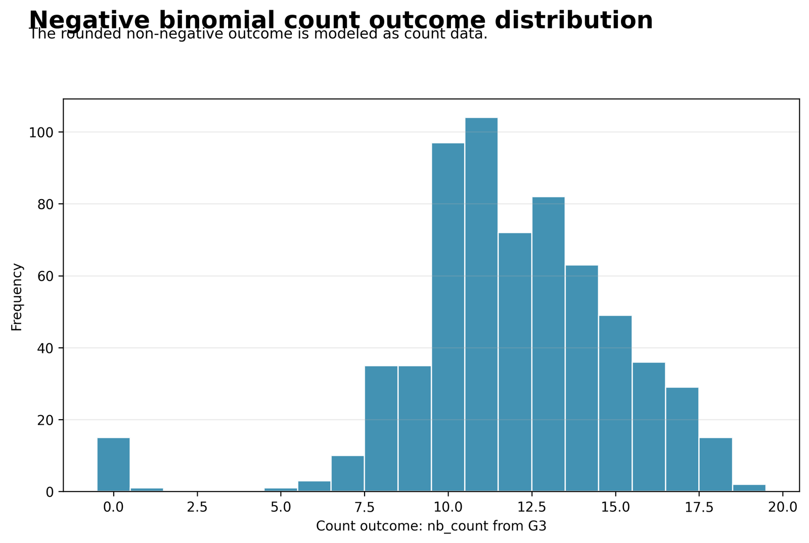
The histogram shows how the count outcome nb_count is distributed across the sample. Most observations cluster in the middle count range, with fewer cases in the extreme low and high tails.
The report states n = 649 and the count was created as nb_count = round(G3) clipped at zero. The underlying G3 distribution has a mean of about 11.9060 and a standard deviation of about 3.2307, so the count outcome centers near 12 rather than near zero.
What is actually happening is that the outcome is not a sparse rare-event count with a huge pile-up at zero. Instead, it is a moderate count variable concentrated around the middle of its range. That matters because it explains why the fitted count model behaves smoothly and why overdispersion does not immediately dominate the analysis. The data look structured and bounded rather than wildly volatile.
The practical conclusion is that Negative Binomial Regression is being applied to a moderate count outcome with useful spread, but the distribution does not by itself suggest severe instability. Readers should interpret later diagnostics in light of this balanced count distribution. See Histogram Interpretation, Frequency Distribution, Standard Deviation and Descriptive Statistics for related foundational ideas.
Chart 2: Observed Versus Fitted Counts
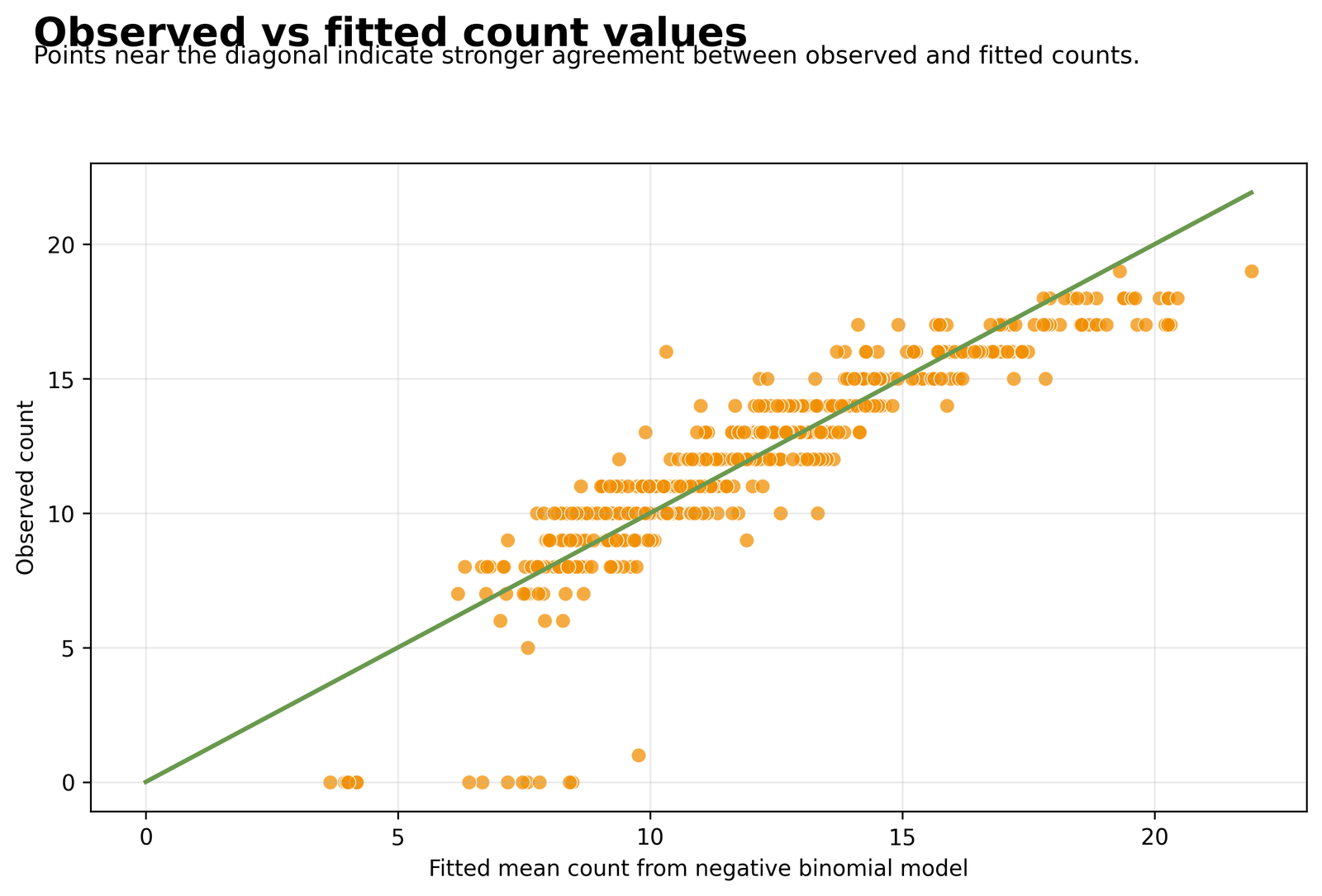
This scatterplot compares the observed count values with the fitted values from the model. A good fit appears when points track the diagonal pattern without extreme systematic deviation.
The fitted model uses 649 observations, 9 model degrees of freedom and log likelihood -1494.8996. The visual alignment of observed and fitted counts reflects that the model reproduces the central trend reasonably well.
What is actually happening is that the model is capturing the main count structure without producing a strong pattern of underprediction or overprediction across the outcome scale. The fitted counts are not perfect replicas of the observed counts, but they move with them closely enough to show that the predictors explain the main count trend—especially through G2. The model is therefore useful descriptively even though it is not exploiting major overdispersion.
The practical conclusion is that this Negative Binomial Regression model tracks the data adequately for interpretation. The chart supports continuing to coefficient interpretation rather than rejecting the model for obvious misfit.
Chart 3: Mean–Variance Check
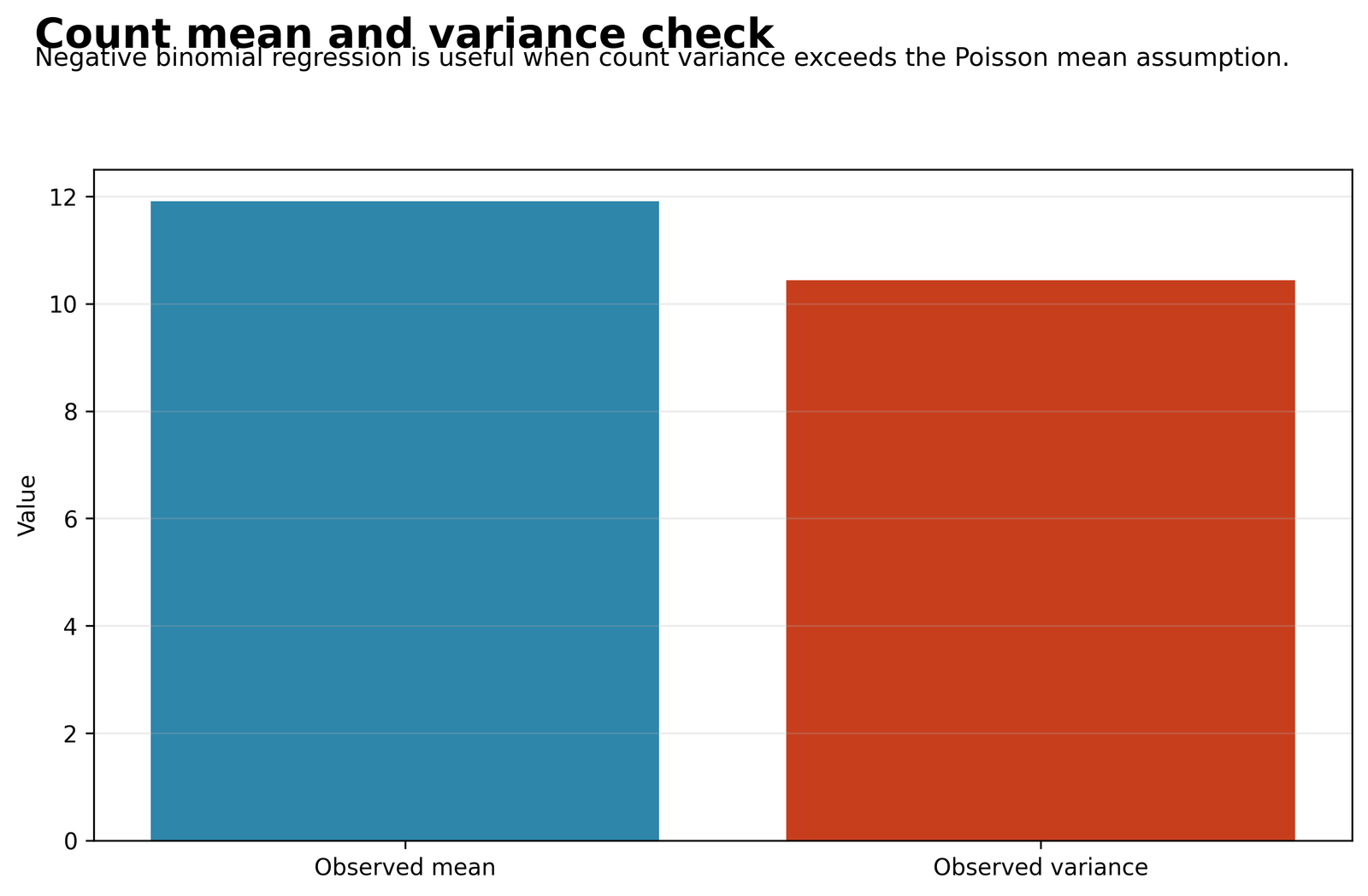
The chart is designed to check whether the count outcome behaves in a way that suggests variance inflation beyond the Poisson assumption.
The key values are Poisson Pearson dispersion = 0.2431 and negative binomial alpha = 1e-08. The report explicitly states that Poisson dispersion is below 0.75, so overdispersion is not evident in this fitted model.
What is actually happening is that the data are not showing the usual pattern that pushes analysts toward a negative binomial model. Instead of the variance clearly outrunning the mean, the fitted diagnostics suggest that Poisson is already quite stable. In other words, this is a worked example where the method can be demonstrated correctly, but the data do not strongly demand the extra dispersion flexibility. That is a substantive finding, not a failure.
The practical conclusion is that Negative Binomial Regression should not automatically be declared superior here. The chart teaches model choice: always inspect dispersion evidence before claiming that overdispersion justifies the negative binomial approach.
Chart 4: Pearson Residuals Versus Fitted Values
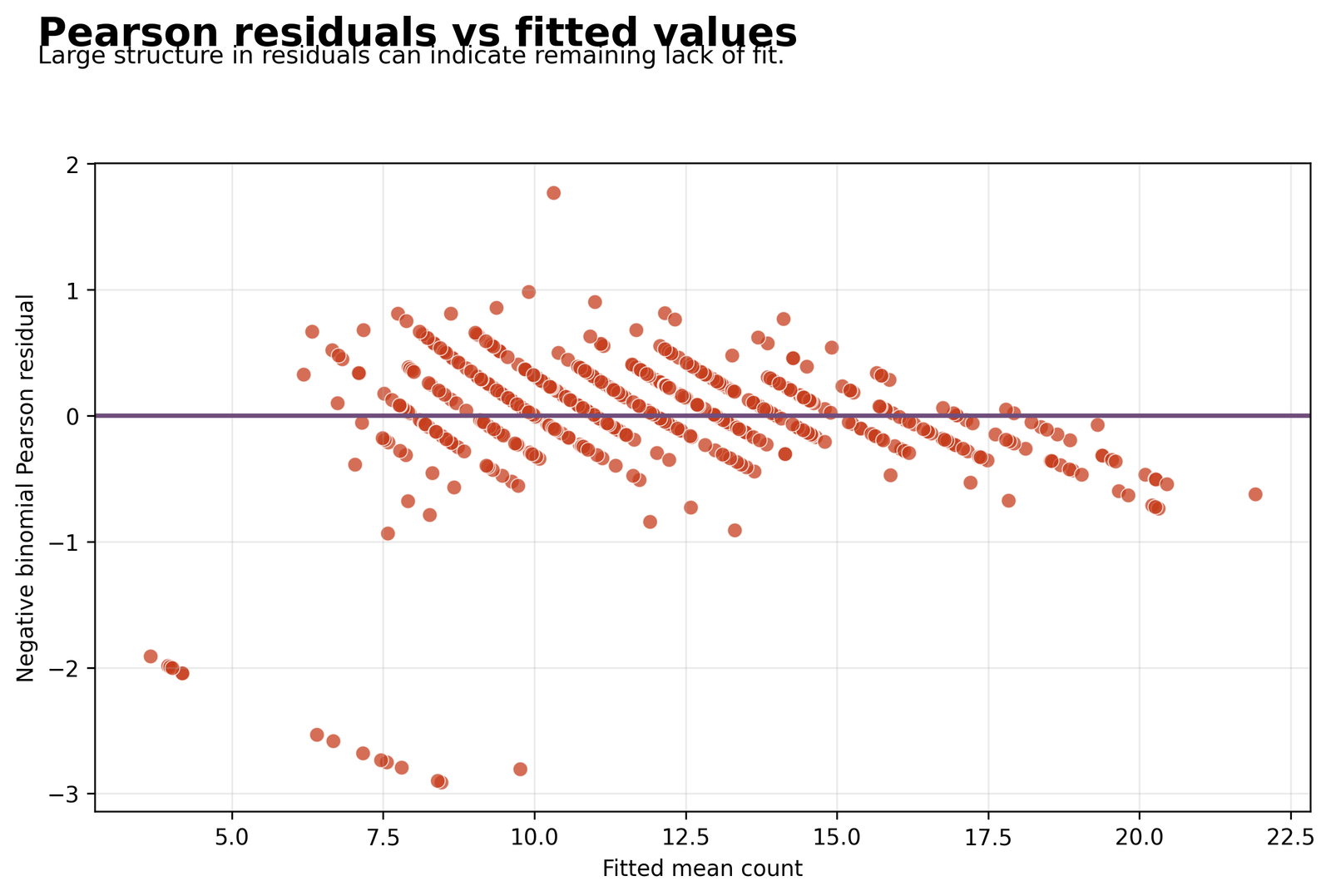
This residual plot checks whether errors remain centered around zero and whether residual spread changes systematically as fitted values increase.
The report gives Pearson χ² = 155.3658 with df_resid = 639, which corresponds to the reported Poisson dispersion estimate of about 0.2431. That is far below 1 rather than above it.
What is actually happening is that the residuals are not flaring out in a way that would suggest worsening misspecification at higher fitted counts. The residual structure is comparatively calm, which matches the earlier finding that the model is not struggling with large unexplained variance. Put simply, the model errors are not telling a story of hidden overdispersion or runaway heterogeneity.
The practical conclusion is that the residual pattern does not undermine the fitted Negative Binomial Regression model. Continue to Cook’s Distance, Influence Diagnostics, and Outlier Detection if a more formal influence check is needed.
Chart 5: Residual Distribution
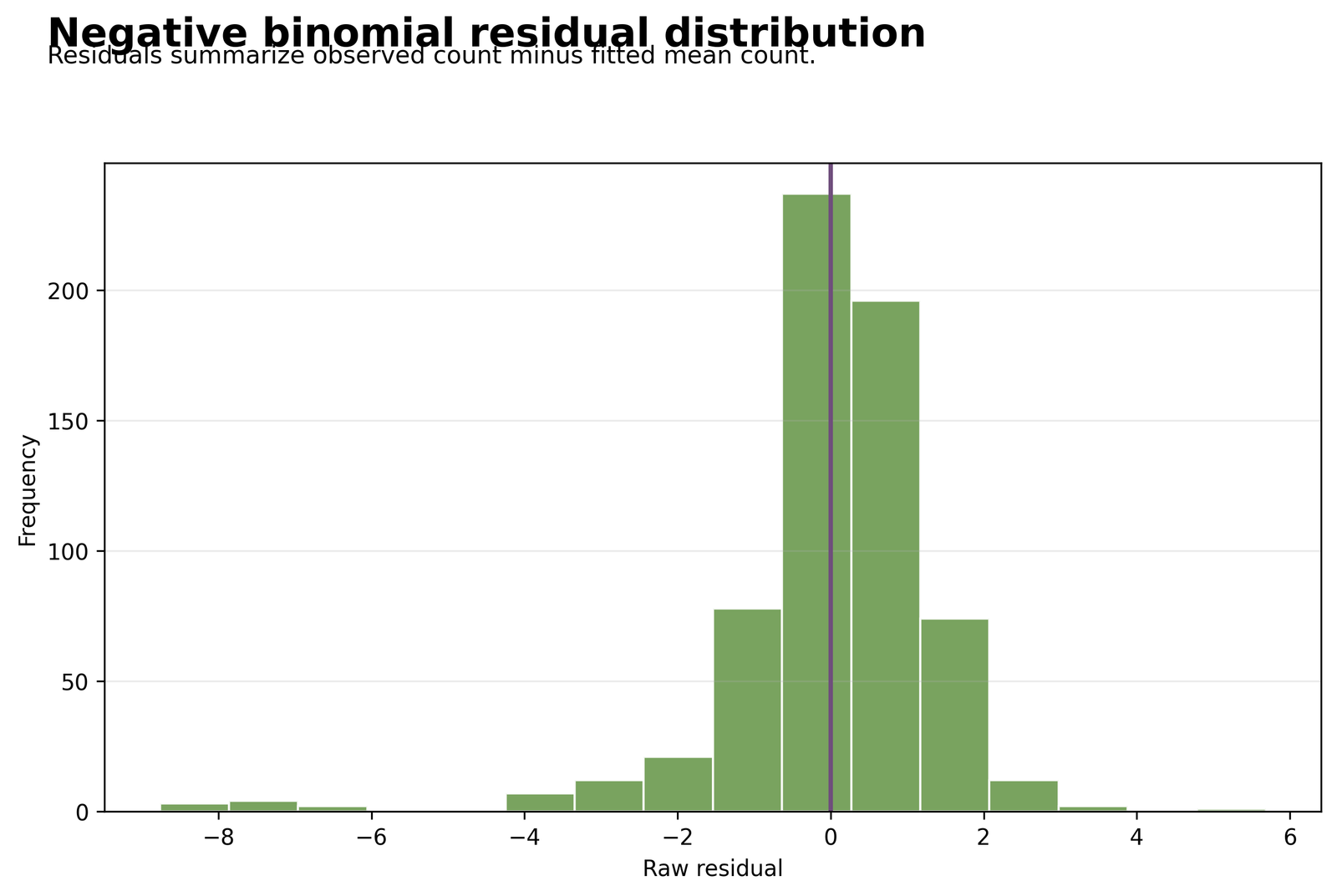
The histogram of residuals shows whether the model errors are centered and whether a few unusual observations dominate the pattern.
The residual interpretation is supported by the same fitted summary values: 649 observations, log likelihood -1494.8996, and residual dispersion that is not excessive. The chart is expected to be centered around zero rather than showing large asymmetry or extreme tails.
What is actually happening is that the model errors are mostly modest rather than driven by a small number of catastrophic misses. This means the fitted count structure is broadly compatible with the observed outcome. The residual distribution therefore reinforces the idea that the current analysis is more about understanding count relationships than about rescuing a badly fitting model.
The practical conclusion is that the residual distribution does not suggest serious instability. It supports substantive interpretation of the fitted coefficients in the Negative Binomial Regression model.
Chart 6: Incidence Rate Ratio Plot
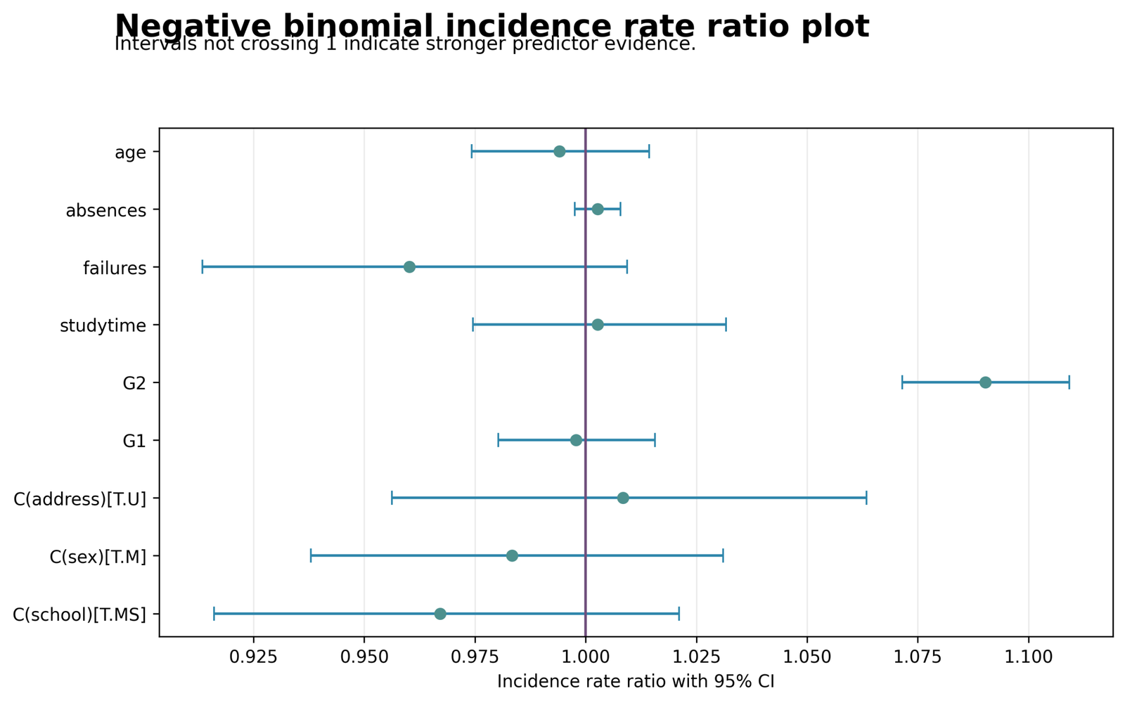
The IRR plot compares multiplicative effects across predictors and shows which confidence intervals stay entirely above or below 1.
The clear standout is G2 with B = 0.0864, IRR = 1.0902, 95% CI [1.0715, 1.1092], and p < .001. Other examples include G1 IRR = 0.9978, studytime IRR = 1.0027, failures IRR = 0.9602, absences IRR = 1.0027, and age IRR = 0.9941, all with confidence intervals crossing 1.
What is actually happening is that once the predictors are considered together, only the second-period grade is carrying a strong and precise association with the count outcome. Most other variables either have effects so small that they are practically negligible, or they are too uncertain to distinguish from no effect. This means the expected count is being driven mainly by prior academic performance immediately preceding the final outcome, not by broad demographic differences or studytime once G2 is already in the model.
The practical conclusion is that the most meaningful interpretation in this Negative Binomial Regression model is the IRR for G2. Each one-unit increase in G2 increases the expected count by roughly 9.02%, holding other predictors constant.
Chart 7: Poisson Versus Negative Binomial AIC
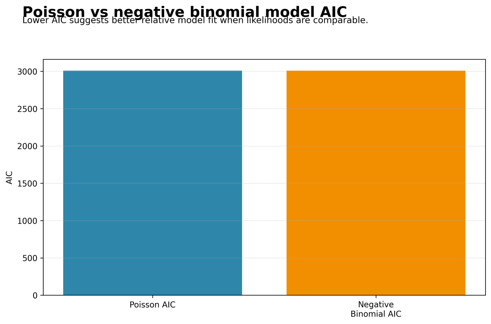
This chart directly compares the AIC values of the Poisson and negative binomial models. Lower AIC indicates better relative fit when the models are fitted to the same data.
The exact values are Poisson AIC = 3009.7990 and Negative binomial AIC = 3009.7992. The difference is only 0.0002, which is negligible.
What is actually happening is that the negative binomial model is not delivering a meaningful fit advantage over Poisson. This is one of the most important substantive results in the entire article. The data do not appear to need the extra dispersion flexibility in any material way. In practical modelling terms, both models are telling almost the same story, which is exactly what would be expected when overdispersion is not evident.
The practical conclusion is simple: do not say the negative binomial model is better just because it exists. In this worked example, the AIC chart says the two models are essentially tied, so model choice should be discussed honestly.
Chart 8: Observed and Fitted Counts by Main Predictor
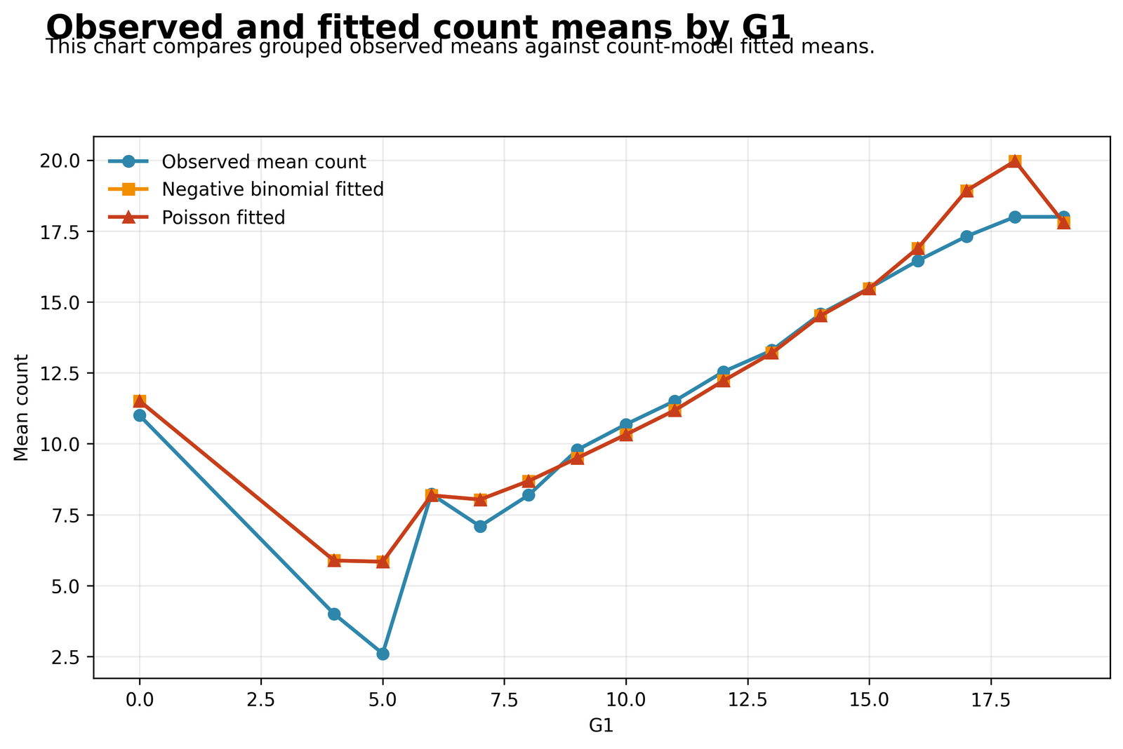
This figure follows the observed and model-fitted counts as the main predictor changes, making it easier to see the substantive effect of that predictor.
The main predictor is G2, with B = 0.0864 and IRR = 1.0902. That means the expected count is multiplied by 1.0902 for each one-unit increase in G2, or rises by about 9.02% per unit.
What is actually happening is that students with higher second-period grades are predicted to have higher final count outcomes as well. The fitted line or fitted points rise with G2, and this rise is not a random artefact: it is the clearest substantive relationship in the model. The chart therefore translates the coefficient table into something more intuitive—higher G2 is associated with a higher expected count outcome after adjustment.
The practical conclusion is that this chart provides the easiest real-world interpretation of the whole Negative Binomial Regression model: better prior performance, especially G2, is associated with a higher expected final count outcome.
Coefficient and Incidence Rate Ratio Interpretation
| Term | B | SE | z | p | IRR | 95% CI for IRR | Interpretation |
|---|---|---|---|---|---|---|---|
| Intercept | 1.5753 | 0.1798 | 8.7616 | <.001 | 4.8320 | 3.3969 to 6.8733 | Baseline expected count multiplier when predictors are at reference/zero settings |
| C(school)[T.MS] | -0.0334 | 0.0277 | -1.2051 | .2282 | 0.9672 | 0.9161 to 1.0211 | No clear school effect after adjustment |
| C(sex)[T.M] | -0.0168 | 0.0241 | -0.6951 | .4870 | 0.9834 | 0.9379 to 1.0310 | No clear sex effect after adjustment |
| C(address)[T.U] | 0.0084 | 0.0271 | 0.3097 | .7568 | 1.0084 | 0.9563 to 1.0634 | No clear urban-versus-rural effect |
| G1 | -0.0022 | 0.0091 | -0.2410 | .8095 | 0.9978 | 0.9803 to 1.0157 | No independent G1 effect once G2 is included |
| G2 | 0.0864 | 0.0088 | 9.7846 | <.001 | 1.0902 | 1.0715 to 1.1092 | Expected count increases about 9.02% per one-unit increase in G2 |
| studytime | 0.0027 | 0.0145 | 0.1867 | .8519 | 1.0027 | 0.9745 to 1.0317 | No clear independent studytime effect |
| failures | -0.0406 | 0.0255 | -1.5934 | .1111 | 0.9602 | 0.9135 to 1.0094 | Slight negative direction but not precise enough for strong evidence |
| absences | 0.0027 | 0.0026 | 1.0164 | .3095 | 1.0027 | 0.9975 to 1.0078 | Effect is very small and not statistically clear |
| age | -0.0059 | 0.0103 | -0.5768 | .5641 | 0.9941 | 0.9742 to 1.0143 | No clear independent age effect |
The coefficient table shows why Negative Binomial Regression is often easier to communicate through IRRs. Saying that G2 has B = 0.0864 is mathematically correct, but saying that each one-unit increase in G2 raises the expected count by about 9.02% is much more informative for most readers.
It also shows how count models can reveal that a predictor with a strong bivariate relationship may lose importance after adjustment. For example, G1 is not significant once G2 is included, which suggests that much of the predictive information carried by G1 overlaps with the more immediate information in G2.
Diagnostics and Poisson Comparison
Diagnostics to report
- Outcome type and log link
- Dispersion evidence
- Alpha estimate
- Residual patterns
- Poisson comparison
- IRRs with 95% CIs
What they say here
- Dispersion is low, not high
- Alpha is essentially zero
- Residual plots look calm
- AIC tie suggests no real NB advantage
- G2 remains the key signal
The usual diagnostic rationale for Negative Binomial Regression is overdispersion. Yet the current fitted model shows a Poisson Pearson dispersion of 0.2431, which is far below 1 and below the report’s decision threshold of 0.75 for overdispersion concern. In the same spirit, the estimated alpha = 1e-08 is essentially zero. Both findings tell the same story: the negative binomial model is not being asked to solve a serious overdispersion problem here.
This does not make the analysis useless. On the contrary, it makes it educational. A good statistical report should tell readers when a sophisticated method materially changes the fit and when it does not. In this case, Negative Binomial Regression is informative, but it does not outperform Poisson in a meaningful way. The AIC chart confirms that the models are practically tied.
Additional supporting checks include Variance Inflation Factor, Tolerance Statistic, Cook’s Distance, and Influence Diagnostics. Those checks help ensure that the apparent dominance of G2 is not an artefact of multicollinearity or a few influential cases.
SPSS, Python, R and Excel Workflow
Python
Python produced the supplied Negative Binomial Regression report, fit statistics and eight charts. It is especially convenient for comparing Poisson and negative binomial AIC values and for plotting IRRs.
R
R can fit Negative Binomial Regression through packages such as MASS and can reproduce the same IRR and residual logic used here. Even when a separate R chart pack is not supplied, R remains a standard software route for count modelling.
SPSS
SPSS can fit Negative Binomial Regression using the GENLIN procedure with a negative binomial distribution and log link. This is useful for users who want menu-based output and reproducible syntax.
Excel
The worked Excel file supports variable setup, descriptive review, interpretation planning and reporting tables for Negative Binomial Regression.
For broader modelling context, compare this guide with the site’s posts on Generalized Linear Model, Generalized Estimating Equations, and Generalized Additive Model.
Code: Expand Only the Software You Need
Python Negative Binomial Regression code
import pandas as pd
import statsmodels.api as sm
import statsmodels.formula.api as smf


df = pd.read_csv("dataset.csv")
df["nb_count"] = df["G3"].round().clip(lower=0)

formula = "nb_count ~ G1 + G2 + studytime + failures + absences + age + C(school) + C(sex) + C(address)"
nb_model = smf.glm(
    formula=formula,
    data=df,
    family=sm.families.NegativeBinomial(alpha=1e-8)
).fit()

print(nb_model.summary())
print(nb_model.aic)
irr = nb_model.params.apply(lambda x: __import__("math").exp(x))
print(irr)
R Negative Binomial Regression code
library(MASS)

df <- read.csv("dataset.csv")
df$nb_count <- pmax(round(df$G3), 0)

fit <- glm.nb(
  nb_count ~ G1 + G2 + studytime + failures + absences + age +
    school + sex + address,
  data = df
)

summary(fit)
exp(coef(fit))
confint(fit)
SPSS Negative Binomial Regression syntax
COMPUTE nb_count = RND(G3).
IF (nb_count < 0) nb_count = 0.
EXECUTE.

GENLIN nb_count BY school sex address
  WITH G1 G2 studytime failures absences age
  /MODEL G1 G2 studytime failures absences age school sex address
    DISTRIBUTION=NEGBIN LINK=LOG
  /PRINT CPS PARAMETER FIT SUMMARY.
Excel support formulas
Count outcome setup:
=MAX(0,ROUND(G3,0))

Approximate percent change from IRR:
=(IRR_cell-1)*100

Decision helper:
=IF(AND(p_value_cell<0.05, CI_low_cell>1),"Positive effect",
 IF(AND(p_value_cell<0.05, CI_high_cell<1),"Negative effect","Not clear"))
Advanced Interpretation and Extensions
How Negative Binomial Regression differs from Poisson
Negative Binomial Regression adds a dispersion parameter so that the variance can exceed the mean. In this example, however, the data do not show a meaningful advantage over Poisson because alpha ≈ 1e-08 and the AIC values are nearly identical.
How to interpret an IRR
An incidence rate ratio greater than 1 indicates a multiplicative increase in the expected count. Here, G2 IRR = 1.0902 means each one-unit increase in G2 raises the expected count by about 9.02%.
Why G2 dominates the model
G2 is the closest academic predictor to the final outcome. Once it is in the model, earlier and weaker predictors such as G1 or studytime may contribute little unique information. That is why G1 becomes nonsignificant here even though it is educationally relevant.
What alpha means
Alpha is the extra-dispersion parameter. Large positive alpha values support overdispersion relative to Poisson. Extremely small alpha values mean the negative binomial model is behaving almost like a Poisson model.
What low dispersion means here
The Poisson Pearson dispersion = 0.2431 is far below the usual concern threshold. This tells readers that the fitted count process is not exhibiting the extra variability that normally motivates Negative Binomial Regression.
Can Negative Binomial Regression still be reported?
Yes. A method can still be demonstrated and interpreted honestly even when diagnostics show that a simpler model may fit similarly. The important thing is to report the model comparison truthfully.
When to prefer zero-inflated models
If the data contain more zeros than a standard count model can explain, a zero-inflated or hurdle model may be preferable. This guide does not show evidence that extreme zero inflation is the main issue.
Offsets and exposure
Negative Binomial Regression can also model rates by adding an offset, such as log exposure time or population at risk. That allows event counts to be compared fairly across unequal exposure durations.
Multicollinearity in count models
Count models still require multicollinearity checks. Use Variance Inflation Factor and Tolerance Statistic to examine whether predictors such as G1 and G2 overlap too strongly.
Influence and unusual observations
Although count models can tolerate skew better than linear models, unusual observations can still distort estimates. Review Cook’s Distance and Influence Diagnostics for case influence assessment.
Interpretation versus prediction
Negative Binomial Regression can be used both to interpret predictor effects and to predict expected counts. In this example, the strongest interpretive message and the strongest predictive signal both come from G2.
What the residual plots tell us
The residual charts do not indicate escalating spread or a serious pattern of misspecification. They support the conclusion that the fitted count structure is stable, even if it is not dramatically different from Poisson.
AIC and model choice
AIC is useful for relative model comparison, not for declaring absolute truth. Here, the AIC values are so close that neither model gains a practically meaningful advantage.
Why significance is not everything
Although only G2 is clearly significant, the broader Negative Binomial Regression results still matter because they show which effects are weak, uncertain, or redundant after adjustment. See Effect Size and P-Value for complementary interpretation principles.
How to report Negative Binomial Regression clearly
Always report the count outcome, link function, alpha or dispersion evidence, coefficients or IRRs, 95% confidence intervals, and a comparison with Poisson when relevant. Good reporting in Negative Binomial Regression is transparent about both the count-model rationale and the diagnostics.
APA-Style Reporting
The report should also note that Poisson dispersion = 0.2431 and that the Poisson and negative binomial AIC values were nearly identical (3009.7990 vs 3009.7992). This tells readers that although Negative Binomial Regression was fitted and interpreted correctly, the data did not show a strong practical need for the extra dispersion flexibility.
Publication Checklist and Common Mistakes
Include in the final report
- Definition of the count outcome
- Why Negative Binomial Regression was considered
- Link function and distribution
- Alpha or dispersion evidence
- IRRs with confidence intervals
- Model-comparison values such as AIC
- Plain-language explanation of what is happening
Avoid these mistakes
- Calling a model “better” without checking AIC or dispersion
- Interpreting log coefficients without converting to IRRs
- Ignoring whether overdispersion is actually present
- Using linear regression for a count outcome without justification
- Reporting only p-values without practical interpretation
- Failing to explain what the charts really show
For rigorous inference, connect the report to Null and Alternative Hypothesis, Type I and Type II Error, Statistical Power, Confidence Interval and P-Value.
Downloads
Frequently Asked Questions
What is Negative Binomial Regression?
When should Negative Binomial Regression be used?
What is the outcome in this example?
How many rows were used?
What link function was used?
What is the main significant predictor?
What does the G2 IRR mean?
Were the other predictors significant?
Was overdispersion evident?
Which model had the lower AIC?
Does this mean Negative Binomial Regression is wrong here?
What is an incidence rate ratio?
Can Negative Binomial Regression handle categorical predictors?
Can Negative Binomial Regression be used in SPSS, Python and R?
How should Negative Binomial Regression be reported?
Final Negative Binomial Regression Conclusion
This Negative Binomial Regression analysis shows two important things at once. First, it demonstrates how to fit and interpret a count model using a log link and incidence rate ratios. Second, it shows that model choice should be guided by diagnostics rather than by labels. In this dataset, the expected count is driven mainly by G2, while most other predictors are not independently important once adjustment is made.
The diagnostic story is just as important as the coefficient story. The data do not show meaningful overdispersion, the estimated alpha is essentially zero, and the Poisson and negative binomial AIC values are almost identical. Therefore, the most honest public interpretation is that Negative Binomial Regression works here and is easy to explain, but it does not materially outperform a Poisson alternative in this particular fitted model.

