Binary outcomes, logit models, odds ratios, discrimination and calibration

Binary Logistic Regression: Formula, Interpretation, SPSS, Python, R and Excel Guide

Binary Logistic Regression predicts the probability of an outcome with two categories. This worked guide models whether a student passed the G3 final-grade threshold, reports exact likelihood, odds-ratio, ROC, calibration and classification results, interprets eight Python charts, validates the model in R, explains the expanded SPSS output and reproduces the calculations in Excel.

649 students549 passes · 100 non-passesAUC 0.9768SPSS · Python · R · Excel

Quick Answer: Binary Logistic Regression Result

The dependent variable is blr_pass, coded 1 when G3 ≥ 10 and 0 when G3 < 10. The Python/R model uses 649 students and nine predictors: G1, G2, studytime, failures, absences, age, school, sex and address.

The overall likelihood-ratio test is significant, χ²(9) = 382.2624, p < .001. McFadden pseudo-R² is 0.6853, Nagelkerke R² is 0.7720, ROC AUC is 0.9768 and accuracy at cutoff 0.50 is 93.53%.

Valid cases649

Pass events549

Sensitivity96.72%

Specificity76.00%

Main conclusion: G1, G2, age and the MS-versus-GP school contrast are significant in the nine-predictor model. G2 is strongest: one additional point multiplies adjusted pass odds by 4.6486.

Calibration qualification: Hosmer-Lemeshow p = .034923 is below .05. The model has excellent discrimination but a statistically detectable calibration concern.

What Is Binary Logistic Regression?
When to Use Binary Logistic Regression
Logit, Probability and Odds-Ratio Formulas
Hypotheses and Decision Rules
Assumptions and Diagnostics
Variables and Data Dictionary
Verified Python/R Results
SPSS Output Interpretation
Eight Python Chart Stories
R Validation Panels
R Model-Fit and Coefficient Tables
Excel Worked File and Formulas
Software Workflows
Code Blocks
APA-Style Reporting
Common Mistakes and Advanced Topics
Downloads
Related Guides
FAQs

What Is Binary Logistic Regression?

Binary Logistic Regression is a regression method for a dependent variable with exactly two mutually exclusive outcomes. It estimates the conditional probability of the category coded 1 and expresses predictor effects on the log-odds scale.

In this analysis, G3 is converted into blr_pass. Students with G3 ≥ 10 are events, and students with G3 < 10 are non-events. The model then estimates how academic, demographic and school variables relate to the adjusted odds of passing.

log[p / (1 − p)] = β₀ + β₁X₁ + β₂X₂ + ··· + βₖXₖ

The model belongs to the Generalized Linear Model family. The binomial distribution describes the binary outcome, and the logit link connects event probability with a linear predictor.

Probability, odds and log odds

Probability	Odds	Log odds	Interpretation
0.10	0.111	−2.197	Event is much less likely than non-event
0.25	0.333	−1.099	One event for roughly three non-events
0.50	1.000	0.000	Event and non-event equally likely
0.75	3.000	1.099	Event odds are three to one
0.90	9.000	2.197	Event is much more likely

Simple definition: Binary Logistic Regression estimates how predictors change the probability and odds that an observation belongs to the event category coded 1.

When to Use Binary Logistic Regression

Outcome structure	Appropriate method	Example
Two unordered categories	Binary Logistic Regression	Pass versus not pass
Three or more unordered categories	Multinomial Logistic Regression	Low, medium or high category
Ordered categories	Ordinal Logistic Regression	Poor, fair, good, excellent
Continuous outcome	Multiple Linear Regression	Predict numeric G3 directly
Count outcome	Poisson Regression or Negative Binomial Regression	Number of absences

Use this method when

The dependent variable has exactly two categories.
The research question concerns adjusted event probability or odds.
Predictors may be continuous, ordinal, binary or categorical.
Discrimination, calibration or classification are relevant outputs.

Do not use the ordinary model when

Observations are clustered or repeated without correlation adjustment.
A predictor combination perfectly separates events and non-events.
Continuous predictors require nonlinear logit effects but only one straight coefficient is fitted.
The outcome has more than two categories or is continuous or count-valued.

For broader method selection, compare Logistic Regression, Multinomial Logistic Regression and Ordinal Logistic Regression.

Binary Logistic Regression Formulas

Logit model

η = log[p / (1 − p)] = β₀ + β₁X₁ + ··· + βₖXₖ

Probability transformation

p = 1 / [1 + exp(−η)]

Odds ratio

OR = exp(B)

A coefficient B represents an adjusted change in log odds. Its exponential is a multiplicative change in odds. OR above 1 indicates higher adjusted event odds, OR below 1 indicates lower adjusted odds, and OR equal to 1 is the null value.

Exact nine-predictor equation

η = −25.3006 − 0.9511schoolMS − 0.6326sexM − 0.0595addressU + 0.6174G1 + 1.5366G2 + 0.1719studytime − 0.3514failures − 0.0433absences + 0.4397age

GP, female and rural are the categorical reference groups. The intercept profile is not substantively realistic because every numeric predictor equals zero, so prediction examples should use realistic student profiles.

Hypotheses and Decision Rules

Test	Null hypothesis	Decision rule
Overall likelihood-ratio test	All slope coefficients equal zero	Reject when p < .05
Individual Wald test	Selected β = 0	Evidence of an effect when p < .05
Odds-ratio interval	OR = 1	An interval excluding 1 supports a nonzero effect
ROC discrimination	AUC = .50	AUC significantly above .50 supports ranking ability
Hosmer-Lemeshow	Grouped observed and expected outcomes agree	A small p-value signals calibration concern

The overall Python/R likelihood-ratio statistic is χ²(9) = 382.2624, p < .001, so the full predictor set fits substantially better than the intercept-only model.

Use Null and Alternative Hypothesis, P-Value and Confidence Interval to interpret the tests without reducing results to a significance label alone.

Assumptions of Binary Logistic Regression

Assumption or check	Meaning in this analysis	Recommended review
Binary dependent variable	blr_pass contains only 0 and 1	Verify G3 threshold coding
Independent observations	Each row represents one student	Use clustered methods if observations are nested or repeated
Linearity in the logit	Continuous effects are linear on log-odds scale	Check transformations, splines or Box-Tidwell terms
No severe multicollinearity	Predictors do not make estimates unstable	Review G1 and G2 with VIF and tolerance
Adequate event information	549 events and 100 non-events	The smaller non-event group limits specificity precision
No separation	Predictors do not perfectly determine the outcome	Use penalized or bias-reduced fitting if separation occurs
No dominating cases	Rare cases should not control the equation	Inspect residuals, leverage and case-deletion influence
Calibration	Predicted probabilities agree with observed rates	Review the significant Hosmer-Lemeshow result

Normal raw predictors and equal outcome variances are not standard requirements. The relevant concerns are event coding, independence, logit linearity, separation, multicollinearity, influential cases, discrimination, calibration and validation.

Review Multicollinearity Check, Variance Inflation Factor, Tolerance Statistic and Influence Diagnostics.

Variables Used and Data Dictionary

Variable	Role	Meaning and coding	Used in
G3	Outcome source	Final grade used to construct the binary dependent variable	All software
blr_pass	Binary dependent variable	1 when G3 ≥ 10; 0 when G3 < 10	All software
G1	Numeric predictor	First-period grade	Python, R and SPSS
G2	Numeric predictor	Second-period grade; strongest fitted predictor	Python, R and SPSS
studytime	Ordinal/numeric predictor	Weekly study-time category	Python, R and SPSS
failures	Numeric predictor	Number of previous class failures	Python, R and SPSS
absences	Numeric predictor	School absence count	Python, R and SPSS
age	Numeric predictor	Student age in years	Python, R and SPSS
school	Categorical predictor	GP reference; MS comparison	Python, R and SPSS
sex	Categorical predictor	Female reference; male comparison	Python, R and SPSS
address	Categorical predictor	Rural reference; urban comparison	Python, R and SPSS
Medu, Fedu, traveltime, health	Additional predictors	Education, travel and health variables	Expanded SPSS model
higher_yes, internet_yes, schoolsup_yes, famsup_yes, paid_yes, activities_yes	Additional dummies	Support, access and activity indicators	Expanded SPSS model

Specification rule: Python and R use nine predictors. The SPSS model adds education, travel, health and support variables. Coefficients from the two specifications should not be presented as though they estimate the same adjusted effect.

Dataset and Verified Python/R Result Summary

Statistic	Python/R result	Interpretation
N	649	All records are used
Events / non-events	549 / 100	84.59% pass and 15.41% non-pass
Log likelihood	−87.7616	Fitted nine-predictor likelihood
Null log likelihood	−278.8928	Intercept-only benchmark
Likelihood-ratio χ²	382.2624, df = 9, p < .001	Predictors substantially improve fit
AIC / BIC	195.5231 / 240.2774	Same-outcome model-comparison indices
McFadden pseudo-R²	0.6853	Large likelihood improvement
Cox-Snell / Nagelkerke R²	0.4451 / 0.7720	Alternative pseudo-R² measures
ROC AUC	0.9768	Excellent discrimination
Hosmer-Lemeshow	χ²(8) = 16.569, p = .034923	Calibration requires review

Complete coefficient and odds-ratio table

Predictor	B	SE	p	Odds ratio	95% CI	Conclusion
school: MS vs GP	−0.9511	0.4352	.0289	0.3863	[0.1646, 0.9066]	Significant lower adjusted odds
sex: M vs F	−0.6326	0.4226	.1344	0.5312	[0.2320, 1.2161]	Not significant
address: U vs R	−0.0595	0.4118	.8851	0.9422	[0.4203, 2.1121]	Not significant
G1	0.6174	0.1397	<.001	1.8542	[1.4101, 2.4380]	Significant positive effect
G2	1.5366	0.2254	<.001	4.6486	[2.9884, 7.2311]	Strongest positive effect
studytime	0.1719	0.2715	.5266	1.1876	[0.6976, 2.0218]	Not significant
failures	−0.3514	0.2518	.1629	0.7037	[0.4296, 1.1528]	Not significant
absences	−0.0433	0.0443	.3283	0.9576	[0.8780, 1.0445]	Not significant
age	0.4397	0.1815	.0154	1.5523	[1.0875, 2.2157]	Significant positive effect

Classification results at cutoff 0.50

Measure	Definition	Result
True negatives	Observed non-pass; predicted non-pass	76
False positives	Observed non-pass; predicted pass	24
False negatives	Observed pass; predicted non-pass	18
True positives	Observed pass; predicted pass	531
Accuracy	(TP + TN) / N	0.9353
Sensitivity	TP / (TP + FN)	0.9672
Specificity	TN / (TN + FP)	0.7600
Precision	TP / (TP + FP)	0.9568
Negative predictive value	TN / (TN + FN)	0.8085
F1 score	2PR / (P + R)	0.9620

Python Report PDFModel fit, coefficients, probabilities and eight charts
SPSS Output PDFExpanded specification, ROC and classification output
Worked Excel FileFormula audit and reporting template

Verified conclusion: G2, G1, age and school_MS have intervals excluding the null odds ratio of 1. The other displayed terms remain compatible with a null adjusted effect at α = .05.

SPSS Output Interpretation for Binary Logistic Regression

The SPSS output fits a broader 19-degree-of-freedom predictor specification. Its stronger fit statistics and altered coefficients reflect the additional education, travel, health and support terms.

Open the Binary Logistic Regression SPSS Output PDF

SPSS fit and classification

SPSS item	Result	Interpretation
Omnibus model test	χ²(19) = 391.774, p < .001	Expanded SPSS model improves over constant-only model
−2 Log Likelihood	166.012	Likelihood-based fit index
Cox & Snell R²	0.453	Pseudo-R² measure
Nagelkerke R²	0.786	Strong likelihood-based fit
Hosmer-Lemeshow	χ²(8) = 19.625, p = .012	Significant grouped calibration discrepancy
Classification	75.0% non-pass; 97.4% pass; 94.0% overall	Model favors pass sensitivity
Confusion counts	TN = 75, FP = 25, FN = 14, TP = 535	610 of 649 classifications correct
ROC AUC	0.979, SE = 0.006, 95% CI [0.967, 0.991]	Excellent discrimination

Selected SPSS coefficients

Predictor	B	p	Exp(B)	95% CI	Conclusion
G1	0.699	<.001	2.012	[1.479, 2.737]	Significant positive predictor
G2	1.555	<.001	4.736	[2.952, 7.596]	Strongest positive predictor
studytime	0.057	.846	1.059	[0.597, 1.877]	Not significant
failures	−0.296	.269	0.744	[0.441, 1.257]	Not significant
absences	−0.047	.316	0.954	[0.871, 1.046]	Not significant
age	0.587	.004	1.799	[1.210, 2.675]	Significant positive predictor
school_MS	−1.178	.017	0.308	[0.117, 0.813]	Lower adjusted odds than GP
sex_M	−0.637	.161	0.529	[0.217, 1.289]	Not significant
address_U	0.031	.945	1.032	[0.422, 2.522]	Not significant
higher_yes	0.968	.070	2.633	[0.925, 7.496]	Positive but not significant at .05

SPSS conclusion: discrimination is excellent, but Hosmer-Lemeshow p = .012 indicates grouped calibration discrepancy. The expanded model should be validated or recalibrated before operational use.

Python Chart-by-Chart Interpretation with Exact Values

Each chart is interpreted through four questions: what is visible, which exact values matter, what the pattern means statistically and what should be checked next.

Python Chart 1: Binary Outcome Distribution

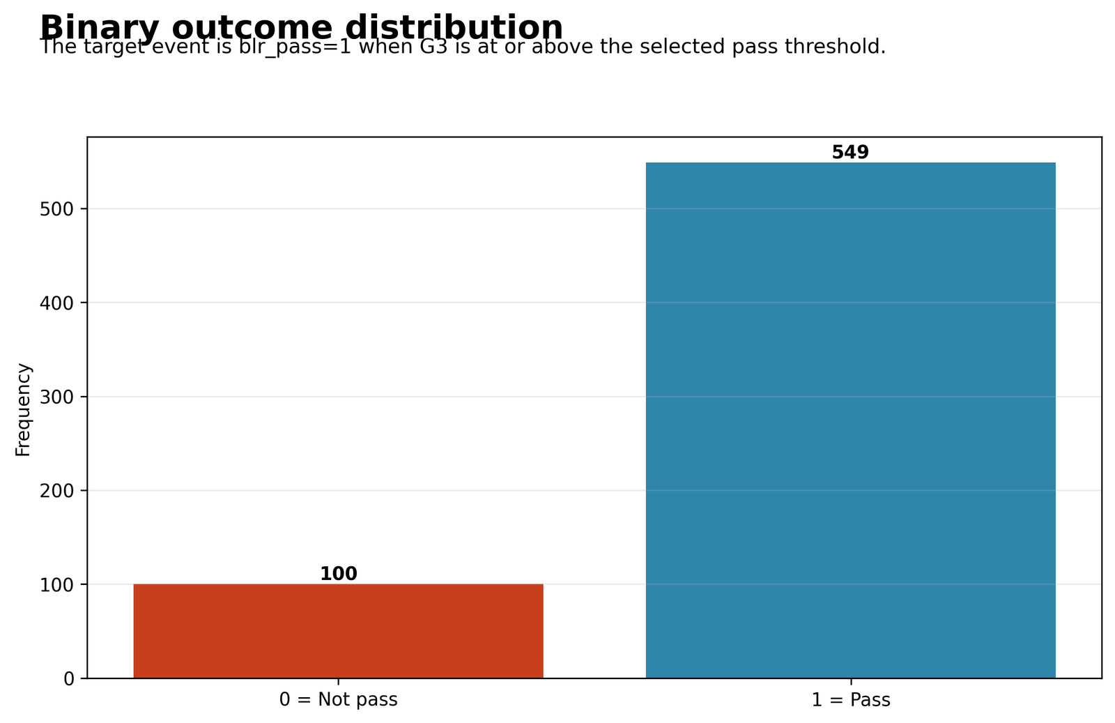
Binary Logistic Regression outcome distribution with 549 passes and 100 non-passes — The dependent variable contains 549 pass events and 100 non-pass cases.

What the chart shows

The chart confirms the exact event coding and displays the class imbalance that affects every classification metric.

Exact values

649 students, 549 passes, 100 non-passes and event prevalence 84.59%.

Statistical meaning

Predicting pass for every student would already achieve 84.59% accuracy. The model must therefore improve non-pass identification as well as overall accuracy.

What to check next

Use specificity and the 100 non-event cases as the main check against a misleading majority-class result.

Binary Logistic Regression cross-check: Python and R reproduce the same nine-predictor estimates, probabilities, ROC AUC and confusion counts.

Python Chart 2: Predicted Probability Distribution by Observed Class

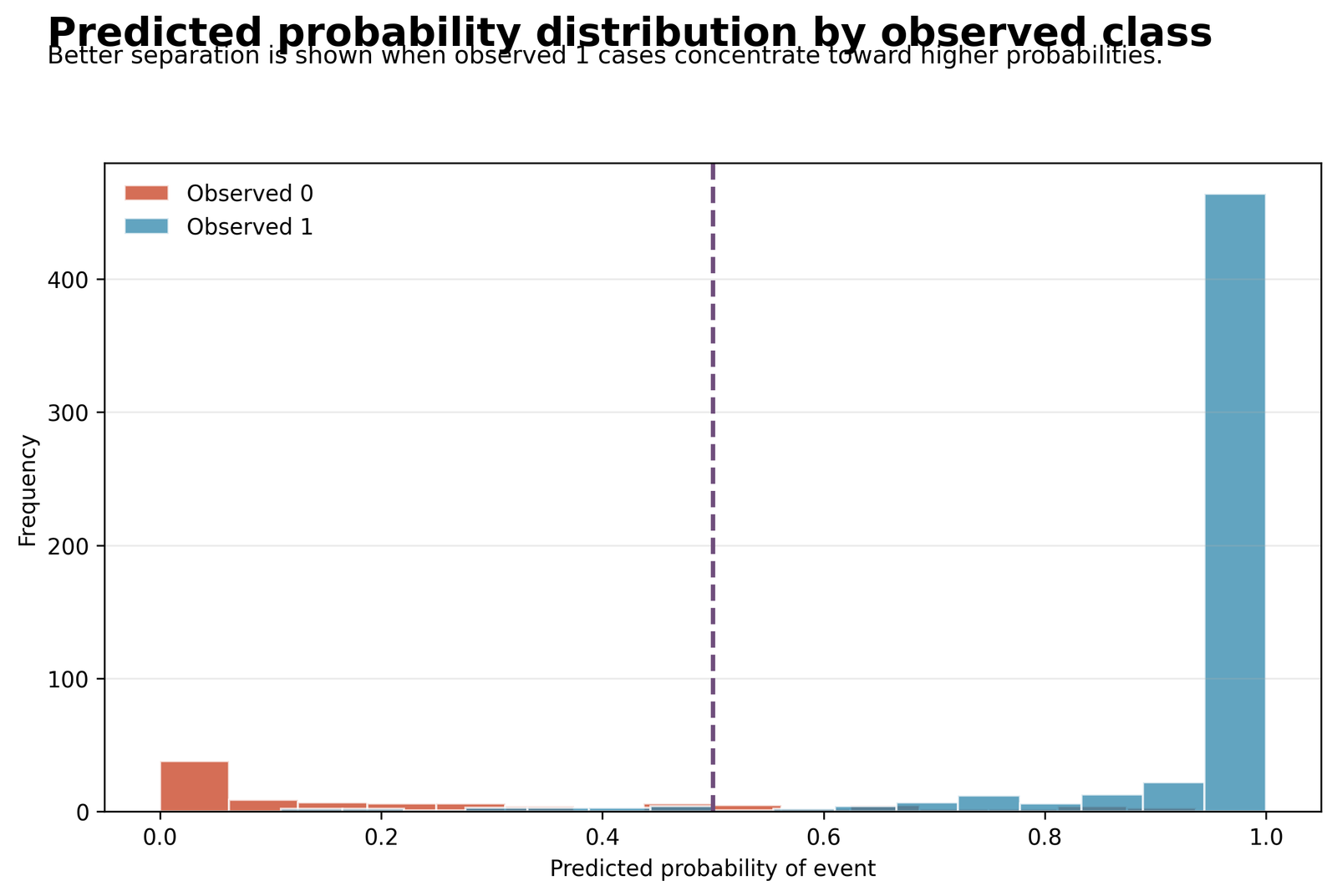
Binary Logistic Regression predicted probability distributions by observed pass class — Pass cases concentrate at high fitted probabilities, while many non-pass cases concentrate near zero.

What the chart shows

The histogram compares predicted pass probabilities for observed passes and non-passes and marks the 0.50 cutoff.

Exact values

76 non-passes fall below 0.50, 24 non-passes fall above it, 531 passes exceed it and 18 passes fall below it.

Statistical meaning

Most observations separate strongly, but the overlapping middle region contains uncertain profiles and all 42 classification errors.

What to check next

Review cases near the threshold and choose the cutoff according to the cost of each error type.

Binary Logistic Regression cross-check: Python and R reproduce the same nine-predictor estimates, probabilities, ROC AUC and confusion counts.

Python Chart 3: ROC Curve and AUC

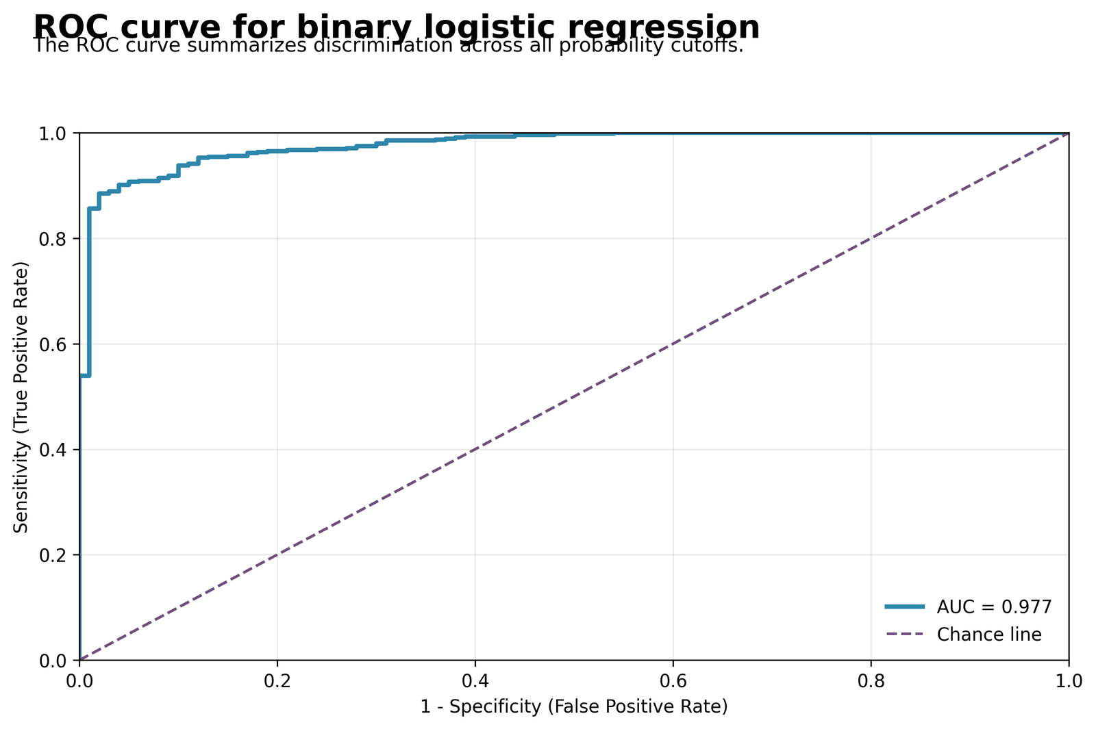
Binary Logistic Regression ROC curve with AUC 0.9768 — The ROC curve evaluates discrimination over all possible probability cutoffs.

What the chart shows

The curve stays close to the upper-left corner, indicating high sensitivity with relatively low false-positive rates.

Exact values

Python/R AUC = 0.9768. SPSS reports AUC = 0.979, SE = 0.006 and 95% CI [0.967, 0.991].

Statistical meaning

A passing student is ranked above a non-passing student approximately 97.68% of the time under the fitted sample.

What to check next

Use AUC for ranking ability, then examine calibration because numerical probabilities can still be biased.

Binary Logistic Regression cross-check: Python and R reproduce the same nine-predictor estimates, probabilities, ROC AUC and confusion counts.

Python Chart 4: Calibration by Predicted-Risk Group

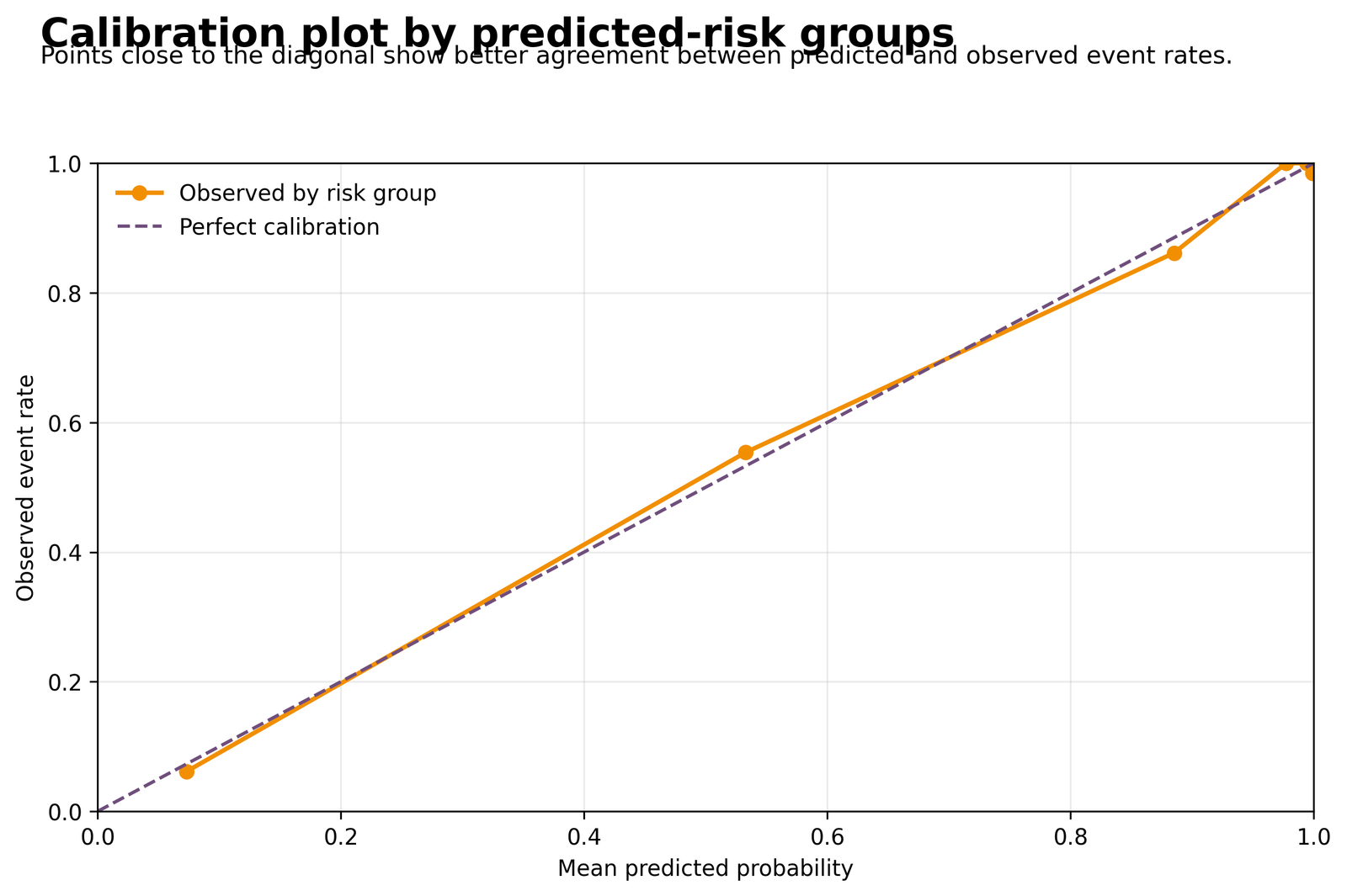
Binary Logistic Regression calibration by predicted probability decile — Grouped mean predictions are compared with observed pass rates.

What the chart shows

The points lie near the diagonal overall, but several groups differ enough to create a statistically detectable lack of fit.

Exact values

Examples include approximately 0.07 predicted versus 0.06 observed, 0.53 versus 0.56, 0.89 versus 0.86 and 1.00 versus 0.98.

Statistical meaning

The model discriminates extremely well but is not perfectly calibrated. Python/R Hosmer-Lemeshow χ²(8) = 16.569, p = .034923.

What to check next

Validate calibration intercept and slope, consider recalibration and avoid describing the probability model as perfect.

Binary Logistic Regression cross-check: Python and R reproduce the same nine-predictor estimates, probabilities, ROC AUC and confusion counts.

Python Chart 5: Odds Ratios with 95% Confidence Intervals

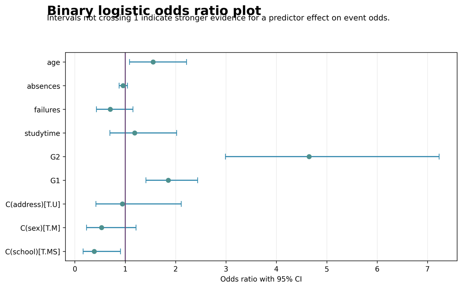
Binary Logistic Regression odds ratio forest plot with confidence intervals — The forest plot compares adjusted odds ratios against the null value of 1.

What the chart shows

The chart displays effect direction, multiplicative magnitude and precision after all nine predictors are included.

Exact values

G2 OR = 4.6486, G1 OR = 1.8542, age OR = 1.5523 and school_MS OR = 0.3863.

Statistical meaning

G2 provides the strongest positive adjusted association. MS students have lower adjusted pass odds than GP students in this fitted model.

What to check next

Translate meaningful predictor changes into fitted probabilities and avoid causal wording.

Binary Logistic Regression cross-check: Python and R reproduce the same nine-predictor estimates, probabilities, ROC AUC and confusion counts.

Python Chart 6: Classification Confusion Matrix

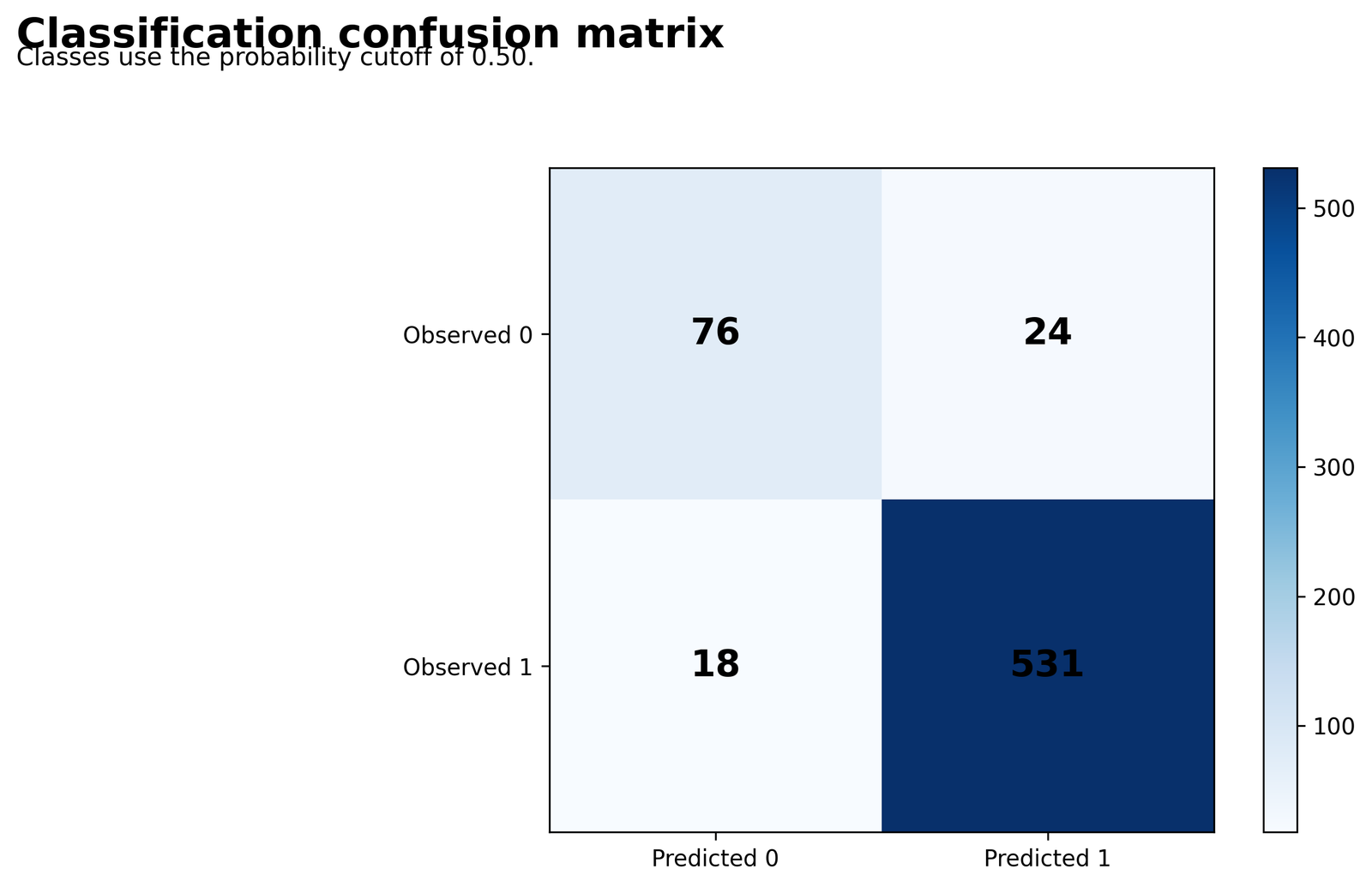
Binary Logistic Regression confusion matrix with 76 true negatives and 531 true positives — The 0.50 cutoff produces 607 correct and 42 incorrect classifications.

What the chart shows

The matrix separates correct and incorrect decisions for the event and non-event groups.

Exact values

TN = 76, FP = 24, FN = 18, TP = 531, accuracy 0.9353.

Statistical meaning

Pass detection is excellent, but 24% of actual non-passes are classified as pass.

What to check next

Adjust the cutoff only after defining whether false positives or false negatives are more costly.

Binary Logistic Regression cross-check: Python and R reproduce the same nine-predictor estimates, probabilities, ROC AUC and confusion counts.

Python Chart 7: Predicted Probability by G2

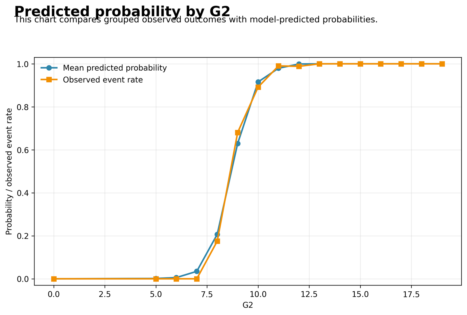
Binary Logistic Regression predicted pass probability by second-period grade G2 — Predicted and observed passing rates rise steeply around G2 values 8 to 11.

What the chart shows

The chart converts the strong positive G2 coefficient into the nonlinear probability scale.

Exact values

Approximate predicted probabilities are 0.21 at G2 = 8, 0.63 at G2 = 9, 0.91 at G2 = 10 and 0.98–0.99 at G2 = 11.

Statistical meaning

A constant log-odds slope creates the largest probability changes near the transition region and smaller changes near probabilities 0 or 1.

What to check next

Report probability contrasts for realistic profiles rather than calling OR 4.6486 a fixed probability increase.

Binary Logistic Regression cross-check: Python and R reproduce the same nine-predictor estimates, probabilities, ROC AUC and confusion counts.

Python Chart 8: Pearson Residuals versus Predicted Probability

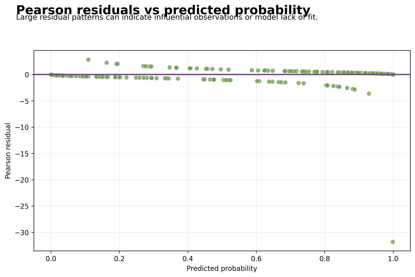
Binary Logistic Regression Pearson residuals versus predicted probability — Most residuals are small, but one high-probability non-pass case has an extreme negative residual.

What the chart shows

The diagnostic plots Pearson residuals against fitted probabilities to locate surprising outcomes.

Exact values

Positive residuals reach roughly +2 to +3. The most extreme negative residual is approximately −32 near a predicted probability of 1.00.

Statistical meaning

The extreme case is a rare outcome relative to the model’s near-certain prediction and may affect fit or calibration.

What to check next

Verify the record, inspect leverage and influence, and test plausible nonlinear or interaction terms before excluding it.

Binary Logistic Regression cross-check: Python and R reproduce the same nine-predictor estimates, probabilities, ROC AUC and confusion counts.

R Chart-by-Chart Validation

The supplied R image references duplicate the Python chart URLs. To avoid presenting the same image twice, the R section uses four paired analytical validation rows built from the exact R results. Each panel is followed by its matching explanation.

R validation pair 1: outcome and probability separation

R outcome distribution

649Complete cases

549Pass events

100Non-events

84.59%Event prevalence

R probability separation

76True negatives

24False positives

18False negatives

531True positives

Explanation for panel above

R outcome validation

R uses the identical blr_pass coding and all 649 observations. The event imbalance is retained rather than artificially balanced.

R conclusion: Compare model accuracy with the 84.59% majority-class benchmark.

Explanation for panel above

R probability-distribution validation

The same 42 cases occupy the wrong side of the 0.50 threshold because R reproduces the same fitted probabilities.

R conclusion: Review borderline cases and report uncertainty rather than treating every class label as equally confident.

R validation pair 2: discrimination and calibration

R discrimination

ROC AUC

0.9768

Accuracy

0.9353

Sensitivity

0.9672

Specificity

0.7600

R calibration evidence

16.569Hosmer-Lemeshow χ²

8Degrees of freedom

0.034923p-value

Calibration concernConclusion

Explanation for panel above

R ROC validation

The R AUC equals 0.9768, confirming excellent ranking discrimination across thresholds.

R conclusion: Do not interpret AUC as evidence that probability values are calibrated.

Explanation for panel above

R calibration validation

The significant grouped lack-of-fit result means that observed and predicted rates differ detectably in at least some risk groups.

R conclusion: Report excellent discrimination together with a calibration qualification.

R validation pair 3: odds ratios and model fit

R key odds ratios

4.6486G2

1.8542G1

1.5523Age

0.3863School_MS

R likelihood summary

−87.7616Log likelihood

382.2624LR χ²(9)

0.6853McFadden R²

195.5231AIC

Explanation for panel above

R odds-ratio validation

R confirms the same direction, magnitude and confidence-interval decisions as Python. G2 remains the dominant adjusted predictor.

R conclusion: Convert odds ratios to probabilities for substantive profiles.

Explanation for panel above

R model-fit validation

The full model improves substantially on the intercept-only likelihood and has strong likelihood-based fit.

R conclusion: Do not describe McFadden R² as ordinary variance explained.

R validation pair 4: main-predictor curve and residual warning

R G2 probability transition

≈ 0.21G2 = 8

≈ 0.63G2 = 9

≈ 0.91G2 = 10

≈ 0.98–0.99G2 = 11

R residual review

≈ +2 to +3Largest positive

≈ −32Extreme negative

Near 1.00Fitted probability

Verify and investigateAction

Explanation for panel above

R G2 probability curve

The R grouped probability pattern reproduces the steep transition around the pass boundary and agrees with OR 4.6486.

R conclusion: Interpret G2 on both the odds and probability scales.

Explanation for panel above

R residual validation

The extreme negative residual identifies a highly surprising non-pass outcome under the fitted profile.

R conclusion: Check data quality, influence, nonlinearity and interactions before considering exclusion.

R Model-Fit and Coefficient Tables

R’s glm(..., family = binomial(link = "logit")) reproduces the Python maximum-likelihood results because the same rows, outcome coding and predictor formula are used.

R model-fit table

R result	Value	Meaning
N	649	All students used
Events / non-events	549 / 100	Pass versus non-pass
Likelihood-ratio χ²	382.2624, df = 9, p < .001	Predictors improve fit
AIC / BIC	195.5231 / 240.2774	Model-comparison indices
McFadden / Nagelkerke R²	0.6853 / 0.7720	Strong likelihood-based fit
ROC AUC	0.9768	Excellent discrimination
Accuracy	0.9353	607 correct classifications
Hosmer-Lemeshow	χ²(8) = 16.569, p = .034923	Calibration warning

R coefficient and odds-ratio table

Term	B	SE	p	Odds ratio	95% CI
school: MS vs GP	−0.9511	0.4352	.0289	0.3863	[0.1646, 0.9066]
sex: M vs F	−0.6326	0.4226	.1344	0.5312	[0.2320, 1.2161]
address: U vs R	−0.0595	0.4118	.8851	0.9422	[0.4203, 2.1121]
G1	0.6174	0.1397	<.001	1.8542	[1.4101, 2.4380]
G2	1.5366	0.2254	<.001	4.6486	[2.9884, 7.2311]
studytime	0.1719	0.2715	.5266	1.1876	[0.6976, 2.0218]
failures	−0.3514	0.2518	.1629	0.7037	[0.4296, 1.1528]
absences	−0.0433	0.0443	.3283	0.9576	[0.8780, 1.0445]
age	0.4397	0.1815	.0154	1.5523	[1.0875, 2.2157]

Excel Worked File and Formula Interpretation

The worked workbook provides an audit trail for outcome coding, linear predictors, probabilities, odds ratios and confusion metrics. The verified Python/R coefficient values should be used when synchronizing the dashboard.

Download the Binary Logistic Regression worked Excel file

Calculation	Excel formula pattern	Purpose
Create pass outcome	`=IF(G3_cell>=10,1,0)`	Creates blr_pass
Linear predictor	`=Intercept+SUMPRODUCT(Coefficients,Predictor_Values)`	Computes η
Predicted probability	`=1/(1+EXP(-Linear_Predictor))`	Converts logit to probability
Predicted class	`=IF(Predicted_Probability>=0.5,1,0)`	Applies cutoff
Odds ratio	`=EXP(Coefficient_B)`	Converts B to Exp(B)
Accuracy	`=(TP+TN)/(TP+TN+FP+FN)`	Overall correct rate
Sensitivity	`=TP/(TP+FN)`	Pass detection
Specificity	`=TN/(TN+FP)`	Non-pass detection
Precision	`=TP/(TP+FP)`	Reliability of predicted passes
F1 score	`=2PrecisionSensitivity/(Precision+Sensitivity)`	Balances precision and sensitivity

Using TN = 76, FP = 24, FN = 18 and TP = 531, Excel should return accuracy 0.9353, sensitivity 0.9672, specificity 0.7600, precision 0.9568, negative predictive value 0.8085 and F1 0.9620.

SPSS, Python, R and Excel Workflows

Software	Main workflow	Primary outputs
SPSS	Create blr_pass, code indicators, run Binary Logistic Regression, request CI for Exp(B), goodness of fit, classification, saved probability and ROC	Omnibus test, pseudo-R², Hosmer-Lemeshow, Exp(B), classification and AUC
Python	Use pandas and statsmodels Logit; calculate ROC, calibration, classification and residuals	Eight PNG charts, tables, text and PDF report
R	Use glm(…, family=binomial(link=’logit’)); calculate ORs, ROC, calibration and confusion metrics	Independent numerical validation and diagnostic tables
Excel	Enter verified coefficients and calculate logits, probabilities, classes and metrics	Worked audit formulas and reporting dashboard

Beginners can review Correlation in Python, Correlation in R, Correlation in SPSS and Correlation in Excel before implementing the full binary model.

Code Blocks for Binary Logistic Regression

SPSS syntax

COMPUTE blr_pass = (G3 >= 10).
VALUE LABELS blr_pass 0 'Not pass' 1 'Pass'.
EXECUTE.

LOGISTIC REGRESSION VARIABLES blr_pass
 /METHOD=ENTER G1 G2 studytime failures absences age
               school_MS sex_M address_U
 /PRINT=GOODFIT CI(95)
 /CRITERIA=PIN(.05) POUT(.10) ITERATE(50) CUT(.5)
 /SAVE=PRED PGROUP COOK LEVER SRESID.

ROC PRE_1 BY blr_pass (1)
 /PLOT=CURVE(REFERENCE)
 /PRINT=SE COORDINATES
 /CRITERIA=CUTOFF(INCLUDE) TESTPOS(LARGE) DISTRIBUTION(FREE) CI(95).

OUTPUT SAVE
 /OUTFILE='D:\DATA ANALYSIS\H Regression Tests and Models\Binary Logistic Regression\SPSS_Output\spv\Binary-Logistic-Regression.spv'.

OUTPUT EXPORT
 /CONTENTS EXPORT=ALL LAYERS=PRINTSETTING MODELVIEWS=PRINTSETTING
 /PDF DOCUMENTFILE='D:\DATA ANALYSIS\H Regression Tests and Models\Binary Logistic Regression\SPSS_Output\pdf\Binary-Logistic-Regression-SPSS-Output.pdf'.

Python code

import numpy as np
import pandas as pd
import statsmodels.formula.api as smf
from sklearn.metrics import (
    roc_auc_score, confusion_matrix,
    accuracy_score, precision_score,
    recall_score, f1_score
)

df = pd.read_csv("dataset.csv")
df["blr_pass"] = (pd.to_numeric(df["G3"]) >= 10).astype(int)

formula = (
    "blr_pass ~ G1 + G2 + studytime + failures + absences + age "
    "+ C(school) + C(sex) + C(address)"
)

model = smf.logit(formula, data=df).fit()
probability = model.predict(df)
predicted = (probability >= 0.50).astype(int)

odds_ratio = np.exp(model.params)
or_ci = np.exp(model.conf_int())

print(model.summary())
print(odds_ratio)
print(or_ci)
print(confusion_matrix(df["blr_pass"], predicted))
print(roc_auc_score(df["blr_pass"], probability))

R code

df <- read.csv("dataset.csv")
df$blr_pass <- ifelse(df$G3 >= 10, 1, 0)

model <- glm(
  blr_pass ~ G1 + G2 + studytime + failures +
    absences + age + school + sex + address,
  data = df,
  family = binomial(link = "logit")
)

probability <- predict(model, type = "response")
predicted <- ifelse(probability >= 0.50, 1, 0)

print(summary(model))
print(exp(coef(model)))
print(exp(confint(model)))
print(table(Observed = df$blr_pass, Predicted = predicted))

Excel formula pattern

Binary outcome:
=IF(G3>=10,1,0)

Linear predictor:
=Intercept+SUMPRODUCT(Coefficients,Predictor_Values)

Predicted probability:
=1/(1+EXP(-Predicted_Logit))

Predicted class:
=IF(Predicted_Probability>=0.5,1,0)

Odds ratio:
=EXP(Coefficient_B)

APA-Style Reporting for Binary Logistic Regression

Python/R report

A Binary Logistic Regression was conducted to predict whether students passed the final-grade threshold. blr_pass was coded 1 when G3 was at least 10 and 0 otherwise. The model included G1, G2, studytime, failures, absences, age, school, sex and address and analyzed 649 students, including 549 passes and 100 non-passes. The model was significant, χ²(9) = 382.26, p < .001, McFadden R² = .685, Nagelkerke R² = .772. Discrimination was excellent, AUC = .977. At cutoff .50, accuracy was 93.53%, sensitivity 96.72% and specificity 76.00%. G2 was the strongest predictor, B = 1.537, OR = 4.649, 95% CI [2.988, 7.231], p < .001. G1, age and the MS-versus-GP school contrast were also significant. Hosmer-Lemeshow χ²(8) = 16.57, p = .035 indicated that calibration should be reviewed.

SPSS report

The expanded SPSS Binary Logistic Regression was significant, χ²(19) = 391.77, p < .001, with Nagelkerke R² = .786. It classified 94.0% of students and achieved AUC = .979, 95% CI [.967, .991]. G1, G2, age and school_MS were significant. Hosmer-Lemeshow χ²(8) = 19.63, p = .012 indicated grouped calibration discrepancy.

Common Mistakes and Advanced Interpretation

Mistake	Why it is a problem	Better practice
Reporting only accuracy	The majority baseline is already 84.59%	Report confusion counts, sensitivity, specificity, precision, F1 and AUC
Interpreting B as an odds ratio	B is a log-odds coefficient	Exponentiate B and report Exp(B)
Treating OR as a probability change	Probability effects depend on baseline risk	Calculate profile-based probability contrasts
Ignoring confidence intervals	A large OR can be imprecise	Report the 95% interval and whether it crosses 1
Calling high AUC perfect fit	Discrimination and calibration differ	Discuss AUC with calibration plots and Hosmer-Lemeshow
Treating pseudo-R² as variance explained	Pseudo-R² is likelihood based	Name and interpret the exact measure
Removing unusual residuals automatically	Rare valid cases can be informative	Verify the case and run sensitivity analysis
Comparing software without checking formulas	SPSS includes additional predictors	State every software specification separately
Ignoring reference categories	Categorical coefficients depend on references	Report GP, female and rural as references
Using cutoff 0.50 automatically	Error costs may not be symmetric	Choose a threshold for the intended decision

Probability, odds and log odds

Probability is bounded between zero and one.
Odds compare event probability with non-event probability.
Log odds extend over the entire real line and form the additive model scale.

Why odds ratios are conditional

Every odds ratio assumes the other variables in the model are held constant.
Adding or removing predictors can change the adjusted odds ratio.
Conditional estimates should not be called simple group differences.

Why probability changes are not constant

The inverse-logit curve is nonlinear.
The same coefficient creates a larger percentage-point change near probability .50 than near 0 or 1.
Profile-based marginal effects are often easier to communicate.

Linearity in the logit

Continuous predictors need not have a linear relationship with probability.
They are assumed linear on the log-odds scale unless transformed.
Splines or polynomial terms can represent curvature.

Interactions

An interaction means one predictor’s log-odds effect depends on another predictor.
Report joint probability contrasts rather than interpreting only the product coefficient.
Use theory and validation to justify added complexity.

Complete separation

Separation occurs when predictor combinations perfectly classify the outcome.
Maximum-likelihood coefficients can diverge.
Penalized or bias-reduced methods may be required.

Pseudo-R-squared measures

McFadden, Cox-Snell and Nagelkerke use different likelihood transformations.
They are not interchangeable with ordinary R-squared.
Always name the exact measure.

Calibration intercept and slope

Ideal calibration has intercept zero and slope one.
A nonzero intercept indicates systematic overprediction or underprediction.
A slope below one often indicates overfitting.

Threshold selection

The default 0.50 cutoff is a convention, not a universal optimum.
Lower cutoffs increase sensitivity and false positives.
Higher cutoffs increase specificity and false negatives.

Internal validation

Apparent performance is optimistic because the fitting sample is reused.
Bootstrap or cross-validation estimates optimism.
All preprocessing and model selection must occur within resamples.

External validation

A new school, cohort or year can have different prevalence and predictor distributions.
AUC, calibration and classification should be reassessed.
Recalibration may be needed even when ranking remains strong.

Class imbalance

Event prevalence is 84.59%.
Accuracy can look high even for a weak majority classifier.
Specificity and confusion counts remain essential.

Influence and unusual cases

Review Cook’s Distance and Influence Diagnostics.
A surprising residual can be valid, erroneous or evidence of omitted structure.
Automatic deletion is not appropriate.

Multicollinearity

Use Multicollinearity Check, Variance Inflation Factor and Tolerance Statistic.
G1 and G2 measure related academic performance.
Strong overlap can widen standard errors without reducing prediction quality.

Robust and clustered inference

Ordinary maximum likelihood assumes independent rows.
Generalized Estimating Equations can estimate population-average effects for correlated binary data.
Mixed-effects logistic models can include cluster-specific random effects.

Penalized Logistic Regression

Elastic Net Regression can stabilize high-dimensional models.
Penalization can reduce variance and handle correlated predictors.
Penalty selection must be validated.

Bayesian Logistic Regression

Bayesian Regression incorporates prior distributions.
Posterior intervals have a different interpretation from confidence intervals.
Weakly informative priors can help with sparse or separated data.

SPSS versus Python/R specifications

The Python/R model uses nine predictors.
The SPSS model adds education, travel, health and support variables.
Different coefficients are expected because the adjusted estimands differ.