
Posterior Inference, Credible Intervals, Bayesian R Squared and Predictive Checking
Bayesian Regression: Interpretation, Python, R, SPSS and Excel Guide
Bayesian Regression combines a likelihood, prior distribution and observed data to produce posterior distributions for regression coefficients, predictions and model-fit quantities. This worked guide uses G3 final grade as the continuous outcome. The full Python and R model uses standardized G1, G2, studytime, failures, absences and age, together with dummy-coded school, sex and address. A separate formula-driven Excel workbook demonstrates the same conjugate Bayesian logic on 25 example rows.
Quick Answer: Bayesian Regression Result
The verified Python and R workflow used 649 complete observations and generated 6,000 posterior draws. The outcome was G3. Numeric predictors were standardized before model fitting, so their coefficients represent the expected movement in G3 for a one-standard-deviation increase in the original predictor while the other model terms are held constant.
The posterior mean Bayesian R squared was 0.8527, with a 95% credible interval from 0.8363 to 0.8678. The posterior mean residual variance was 1.5404. Predictions based on posterior mean fitted values had RMSE = 1.2410 and MAE = 0.7801.
Final interpretation: the posterior distribution indicates strong predictive fit for G3. Standardized G2 has the largest positive posterior coefficient, followed by standardized G1. Standardized failures has a negative credible effect, and the M-coded sex indicator also has a small negative 95% credible interval. Studytime, absences, age, school and address have intervals that cross zero in this specification.
Do not mix the two model specifications: the Python/R model uses all 649 rows and nine predictors after standardization and dummy coding. The Excel workbook is a separate 25-row teaching example using only standardized G1, G2, studytime and failures. Its coefficient values are therefore not expected to equal the full-data results.
Table of Contents
- What Is Bayesian Regression?
- When to Use Bayesian Regression
- Likelihood, Prior and Posterior Formula
- How to Interpret Bayesian Regression
- Dataset and Variables Used
- Posterior Coefficient Results
- Python Chart-by-Chart Interpretation
- R Charts, Tables and Independent Validation
- SPSS Output Interpretation
- Excel Worked Results Explained
- Python, R, SPSS and Excel Workflows
- Bayesian Regression Code
- APA-Style Reporting
- Common Mistakes
- Downloads and Resources
- Related Guides
- FAQs
What Is Bayesian Regression?
Bayesian Regression is a regression framework in which unknown coefficients and model parameters are represented by probability distributions. Before seeing the data, the researcher specifies a prior distribution. The likelihood describes how the observed outcome is generated conditional on the predictors and parameters. Bayes’ theorem combines the prior and likelihood to create the posterior distribution.
A conventional regression table usually reports one estimate, one standard error, a confidence interval and a p-value. Bayesian output instead gives a complete posterior distribution for each coefficient. This allows the researcher to report the posterior mean, posterior median, posterior standard deviation, a 95% credible interval and the posterior probability that the coefficient has a positive or negative direction.
Simple definition: Bayesian regression updates prior beliefs about regression coefficients with the information contained in the observed data. The result is a posterior distribution that quantifies both effect direction and uncertainty.
When to Use Bayesian Regression
Bayesian regression is useful when direct probability statements about parameters are valuable, when prior information should be incorporated, when samples are limited, when complex hierarchical models are needed, or when prediction uncertainty must be propagated through the complete model.
| Research Situation | Why Bayesian Regression Helps | Example Interpretation |
|---|---|---|
| You want a probability statement about a coefficient. | The posterior directly measures uncertainty about coefficient direction and magnitude. | There is a 99% posterior probability that the failures coefficient is negative. |
| You have meaningful prior information. | Priors formally combine previous evidence with current data. | A previous study can inform a weakly informative prior for a grade predictor. |
| You need posterior predictive intervals. | Predictions integrate uncertainty in coefficients and residual variance. | A future G3 score receives a full predictive distribution rather than one point estimate. |
| You are fitting a complex model. | Bayesian methods extend naturally to multilevel, nonlinear and latent-variable settings. | School-level random effects can be included in a hierarchical Bayesian regression. |
| You only need a simple large-sample linear model. | Bayesian regression remains valid, but classical regression may be simpler if prior and posterior interpretation add no value. | Use the approach that best matches the reporting question. |
Bayesian Regression Likelihood, Prior and Posterior Formula
The worked model uses a normal linear likelihood:
The coefficient prior is conditionally normal, and the variance prior is inverse gamma:
For this analysis, the prior mean is zero, the intercept prior variance is 1000, the slope prior variance is 100, and the inverse-gamma settings are a₀ = 2 and b₀ = 2. These are broad priors relative to the standardized predictor scale.
Posterior Updating
The posterior distribution combines prior precision and data precision. With 649 observations, the likelihood contributes substantial information, so the posterior for the strongest grade predictors is narrow.
Bayesian R Squared
Bayesian R squared is calculated for each posterior draw. The final output is therefore a distribution rather than one fixed number. In this model, the posterior mean is 0.8527 and the central 95% credible interval is 0.8363 to 0.8678.
How to Interpret Bayesian Regression Results
The most important Bayesian quantities are the posterior mean, posterior standard deviation, credible interval, probability of direction and posterior predictive distribution.
| Bayesian Output | Meaning | Interpretation Rule |
|---|---|---|
| Posterior mean | Average coefficient across posterior draws. | Use it as the central estimate while retaining the uncertainty interval. |
| Posterior SD | Spread of the coefficient posterior. | Smaller values indicate greater posterior precision. |
| 95% credible interval | Interval containing 95% of the posterior coefficient draws. | An interval fully above or below zero provides stronger evidence for a directional effect. |
| Probability of direction | Larger of P(β > 0) and P(β < 0). | Values near 1 show high posterior certainty about the sign. |
| Posterior predictive check | Comparison between observed data and replicated outcomes drawn from the fitted model. | The replicated distribution should reproduce important features of the observed distribution. |
| Bayesian R² | Posterior distribution for explained outcome variance. | Report its posterior mean and credible interval. |
Credible interval is not a frequentist confidence interval: a 95% Bayesian credible interval is interpreted through the posterior distribution under the stated model and prior. It should not be described using repeated-sampling confidence-interval wording.
Dataset and Variables Used
The full Python and R workflow uses the student-performance data with G3 as the continuous outcome. Six numeric predictors are standardized, and three categorical variables are dummy coded. The standardization step places numeric predictors on a comparable scale and improves posterior computation.
Full Python and R Model Variable Dictionary
| Variable | Model Role | Plain-English Meaning / Coding | Coefficient Interpretation |
|---|---|---|---|
| G3 | Continuous outcome | Final grade, ranging from 0 to 19 in the analyzed data. | The model predicts the posterior distribution of final grade. |
| z_G1 | Standardized predictor | First-period grade transformed to mean 0 and SD 1. | Expected G3 change for a one-SD increase in G1. |
| z_G2 | Standardized predictor | Second-period grade transformed to mean 0 and SD 1. | Expected G3 change for a one-SD increase in G2. |
| z_studytime | Standardized predictor | Weekly study-time category on a standardized scale. | Adjusted G3 movement for a one-SD increase in studytime. |
| z_failures | Standardized predictor | Number of previous class failures on a standardized scale. | Adjusted G3 movement for a one-SD increase in failures. |
| z_absences | Standardized predictor | School absence count on a standardized scale. | Adjusted G3 movement for a one-SD increase in absences. |
| z_age | Standardized predictor | Student age on a standardized scale. | Adjusted G3 movement for a one-SD increase in age. |
| school_MS | Dummy predictor | 1 = MS school; 0 = GP reference school. | Adjusted G3 difference between MS and GP. |
| sex_M | Dummy predictor | 1 = M; 0 = F reference group. | Adjusted G3 difference for the M-coded group. |
| address_U | Dummy predictor | 1 = urban; 0 = rural reference group. | Adjusted G3 difference for urban versus rural address. |
Excel Workbook Variable Dictionary
The Excel workbook contains 25 example rows. It predicts G3 from an intercept and four standardized predictors: G1, G2, studytime and failures. It does not include absences, age or categorical dummy variables. The Excel results must therefore be presented as a separate worked example.
Posterior Coefficient Results for the 649-Row Model
The consolidated posterior table below is shared by the Python and R interpretations. A predictor is labelled a credible effect when its 95% credible interval does not cross zero.
| Term | Posterior Mean | Posterior SD | 95% Credible Interval | Probability of Direction | Decision |
|---|---|---|---|---|---|
| Intercept | 11.9774 | 0.1202 | 11.7401 to 12.2129 | 1.0000 | Credible baseline |
| z_G1 | 0.3654 | 0.0971 | 0.1771 to 0.5535 | 1.0000 | Credible positive effect |
| z_G2 | 2.5623 | 0.0965 | 2.3715 to 2.7479 | 1.0000 | Credible positive effect |
| z_studytime | 0.0522 | 0.0520 | -0.0487 to 0.1547 | 0.8405 | Interval crosses zero |
| z_failures | -0.1343 | 0.0560 | -0.2445 to -0.0238 | 0.9900 | Credible negative effect |
| z_absences | 0.0831 | 0.0509 | -0.0169 to 0.1813 | 0.9492 | Interval narrowly crosses zero |
| z_age | 0.0283 | 0.0524 | -0.0743 to 0.1316 | 0.7043 | Interval crosses zero |
| school_MS | -0.1647 | 0.1151 | -0.3905 to 0.0599 | 0.9207 | Interval crosses zero |
| sex_M | -0.2052 | 0.1033 | -0.4077 to -0.0032 | 0.9763 | Small credible negative effect |
| address_U | 0.1009 | 0.1134 | -0.1192 to 0.3277 | 0.8150 | Interval crosses zero |
The dominant coefficient is z_G2 = 2.5623. Because G2 is standardized, a one-standard-deviation increase in second-period grade is associated with an expected increase of about 2.56 G3 points, conditional on the remaining variables. The next credible academic effect is z_G1 = 0.3654. Previous failures and the M-coded sex indicator have negative intervals fully below zero, although their magnitudes are much smaller than the G2 effect.
Python Chart-by-Chart Interpretation with Real Posterior Values
The Python generator creates eight charts. The discussion below integrates the exact model values into the narrative rather than adding a separate data table below every figure.
Python Chart 1: G3 Outcome Distribution
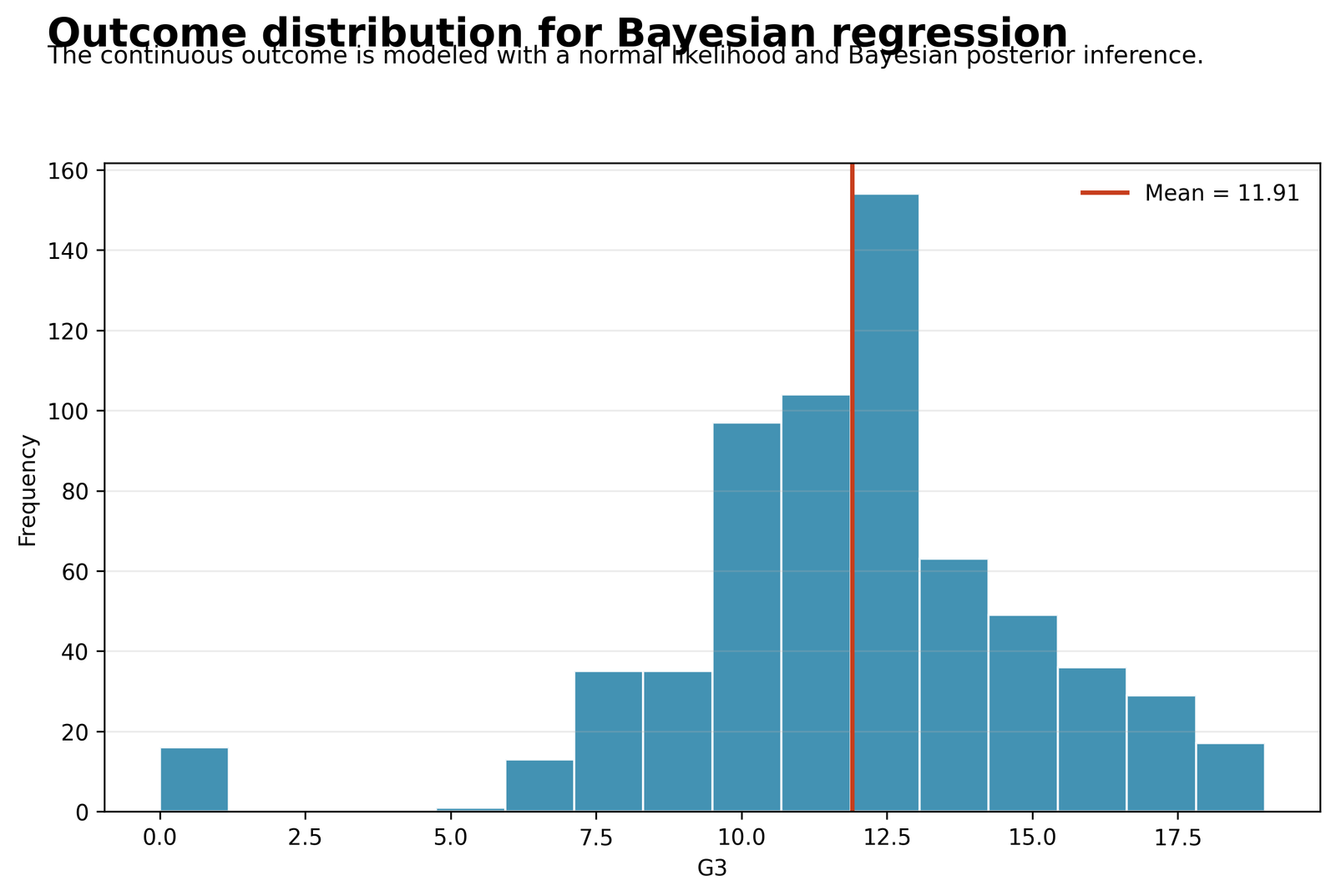
The model uses 649 G3 scores. The mean is 11.9060, the median is 12, the standard deviation is 3.2307, and the observed range is 0 to 19. The middle 50% of scores lies from 10 to 14. The most frequent outcomes are G3 = 11 with 104 students, G3 = 10 with 97 students, G3 = 13 with 82 students, and G3 = 12 with 72 students.
The distribution is concentrated in the central grade range but includes 15 zero scores and only 2 scores of 19. The normal likelihood is an approximation for this bounded integer outcome. The posterior predictive check is therefore essential because strong regression fit does not automatically guarantee that every feature of the observed grade distribution is reproduced.
Python Chart 2: Posterior Coefficient Credible Intervals
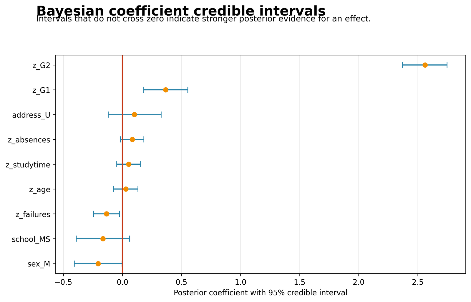
Four predictor intervals remain fully away from zero. The largest is z_G2 = 2.5623 with a 95% credible interval of 2.3715 to 2.7479. The interval for z_G1 = 0.3654 is 0.1771 to 0.5535. The negative credible effects are z_failures = -0.1343, interval -0.2445 to -0.0238, and sex_M = -0.2052, interval -0.4077 to -0.0032.
The remaining intervals cross zero: studytime from -0.0487 to 0.1547, absences from -0.0169 to 0.1813, age from -0.0743 to 0.1316, school_MS from -0.3905 to 0.0599, and address_U from -0.1192 to 0.3277. This chart shows why coefficient magnitude, posterior uncertainty and direction probability should be interpreted together.
Python Chart 3: Observed vs Posterior Fitted Values
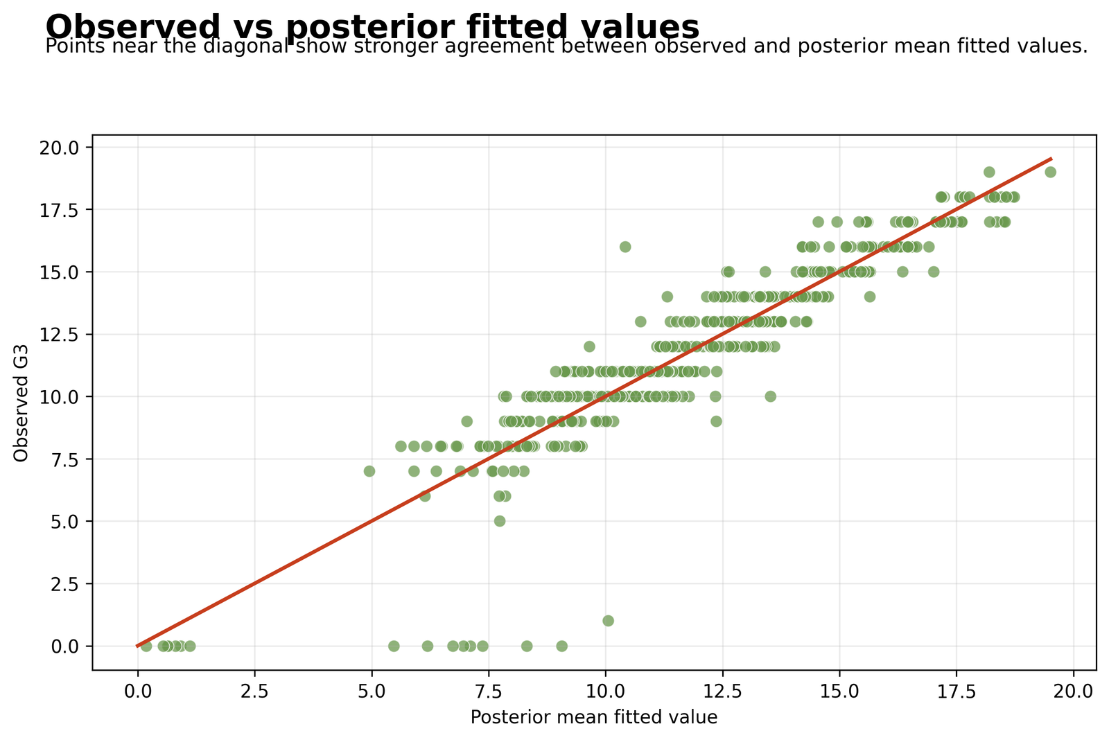
The correlation between observed G3 and posterior mean fitted values is approximately 0.9232. The fitted values range from about 0.1768 to 19.5107, while observed G3 ranges from 0 to 19. The model has RMSE = 1.2410 and MAE = 0.7801, indicating that the typical absolute error is below one grade point even though several extreme cases are predicted less accurately.
Most observations cluster around the 45-degree agreement line, especially in the middle of the grade scale. Horizontal bands occur because G3 is recorded in integer values while fitted means are continuous. The strongest deviations are low observed grades that receive higher fitted values, which also create the long negative residual tail in Chart 4.
Python Chart 4: Posterior Mean Residual Distribution
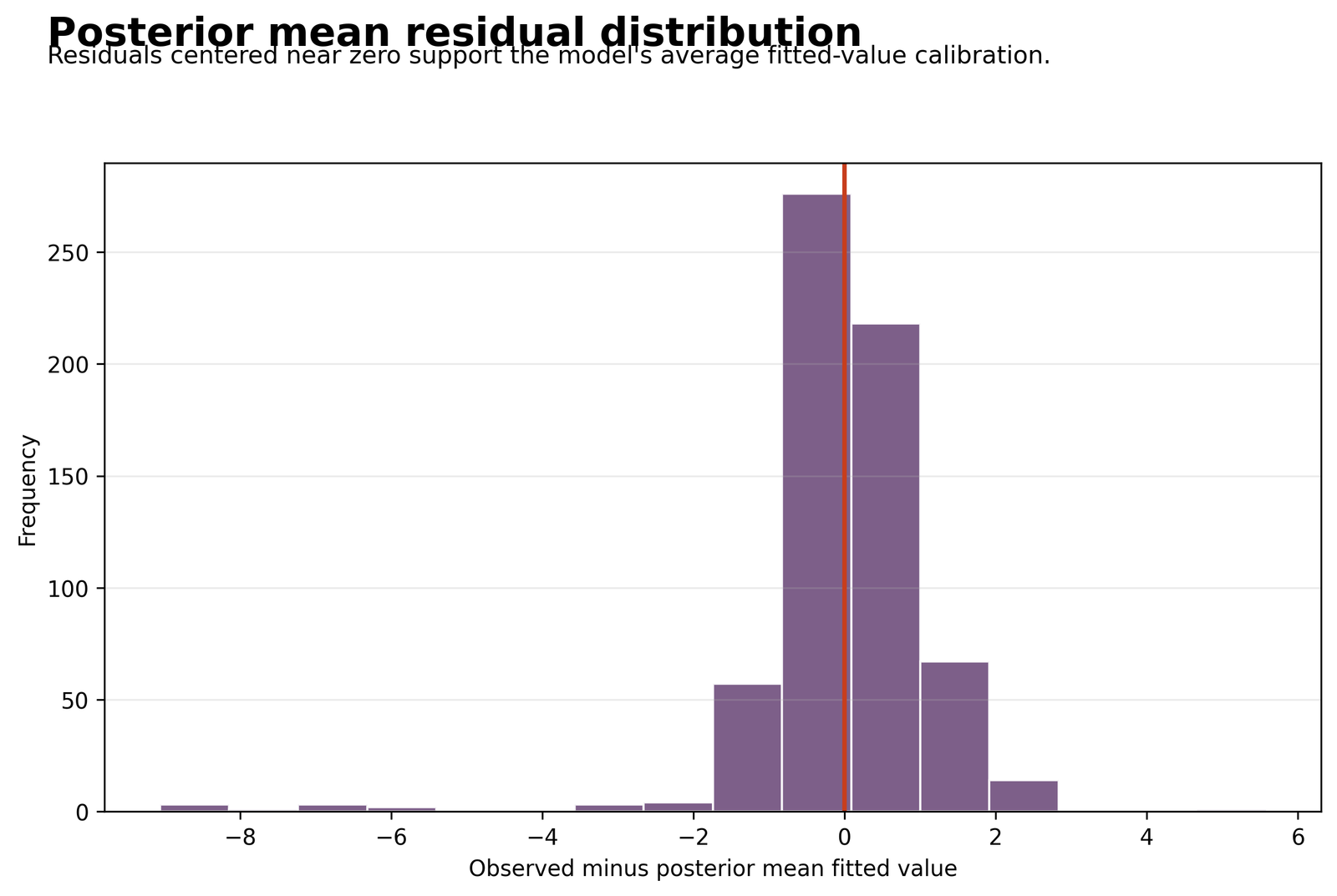
The residual mean is approximately -0.0002, so the average posterior fitted value is well calibrated to the observed mean. The residual standard deviation is 1.2419. The first quartile is -0.4848, the median is -0.0377, and the third quartile is 0.6506.
The residual range is asymmetric: the minimum is -9.0625 and the maximum is 5.5799. The central mass is close to zero, but the extreme negative tail reveals students whose observed G3 is much lower than the model predicts. These cases should be examined using studentized residuals, Cook’s distance, influence diagnostics and outlier detection.
Python Chart 5: Posterior Predictive Check
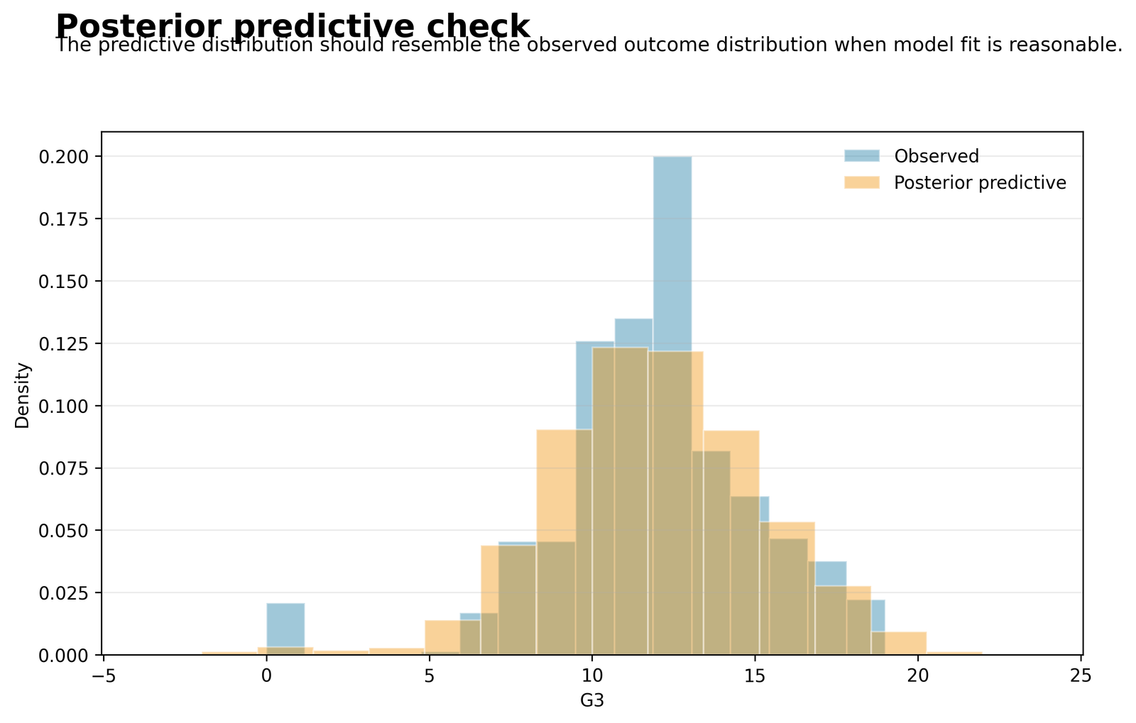
The observed mean is 11.9060 and the posterior replicated mean is approximately 11.9084. The observed standard deviation is 3.2307, while the pooled replicated standard deviation is approximately 3.2319. This close agreement shows that the fitted model reproduces the overall location and spread of G3.
The central 95% observed range is approximately 5.2 to 17.8. The posterior predictive central 95% range is about 5.84 to 18.22. The predictive distribution is slightly smoother and extends beyond the observed integer support because the model uses a continuous normal likelihood. The check supports broad calibration, while the zero-score mass and bounded scale remain features to discuss.
Python Chart 6: Bayesian R Squared Posterior Distribution
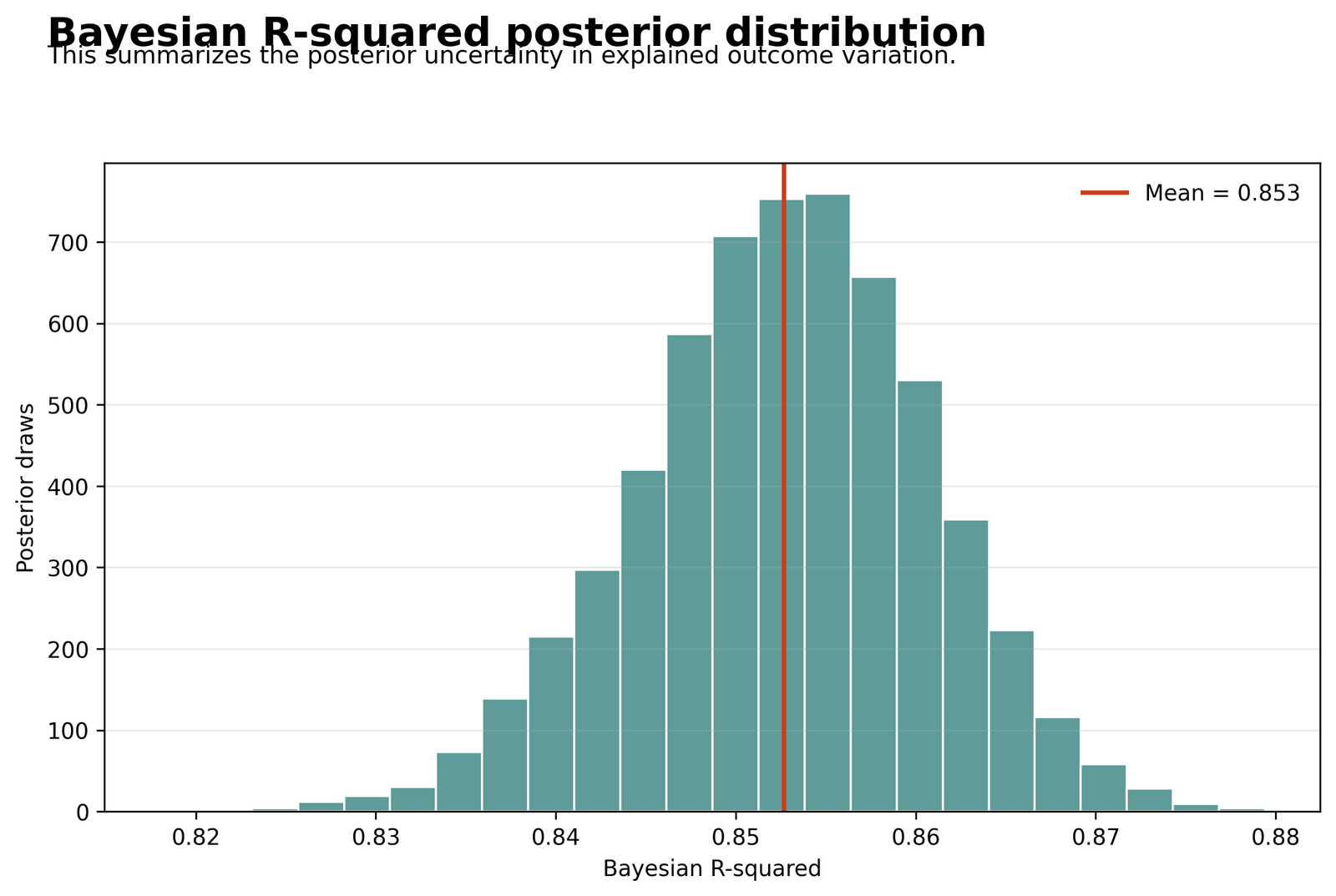
The Bayesian R squared posterior is centered at 0.8527. Its 95% credible interval is 0.8363 to 0.8678. This means that, under the stated likelihood and priors, the posterior places 95% of the central R squared mass within that interval.
The narrow interval reflects the large sample and the strong information carried by G1 and G2. Bayesian R squared should still be interpreted as in-sample explained variation. It does not replace out-of-sample validation, posterior predictive diagnostics or assessment of influential observations.
Python Chart 7: Posterior Distribution for the Top Coefficient
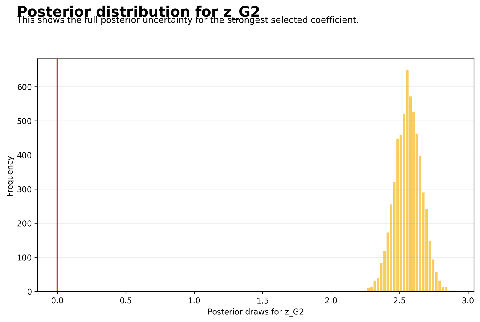
The strongest coefficient is z_G2. Its posterior mean is 2.5623, posterior median is 2.5631, posterior SD is 0.0965, and 95% credible interval is 2.3715 to 2.7479. All 6,000 sampled values are positive to the displayed precision, so its probability of direction is 1.0000.
Because G2 is standardized, the coefficient means that a one-standard-deviation increase in second-period grade is associated with an expected increase of about 2.56 final-grade points after controlling for the other numeric and categorical predictors. The narrow posterior indicates much greater precision than for the smaller contextual variables.
Python Chart 8: Probability of Coefficient Direction
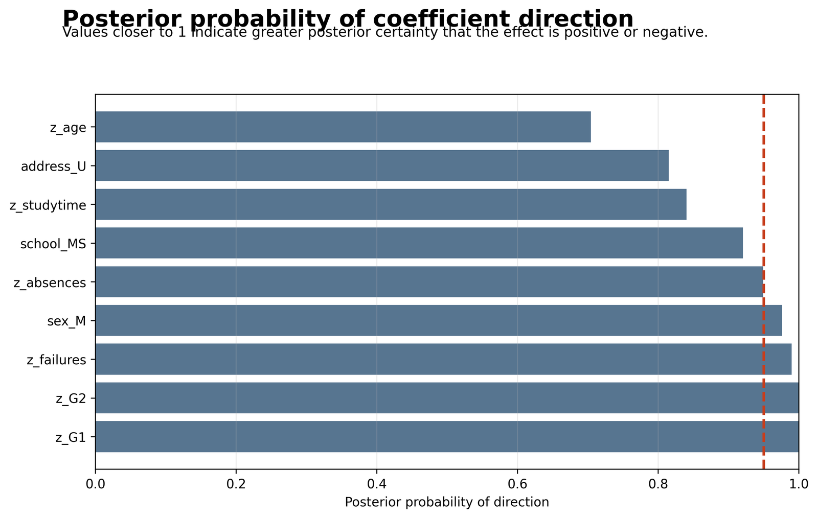
The highest direction probabilities are 1.0000 for z_G1 and 1.0000 for z_G2, followed by 0.9900 for z_failures, 0.9763 for sex_M, 0.9492 for z_absences, and 0.9207 for school_MS. Studytime has 0.8405, address_U has 0.8150, and age has 0.7043.
A high direction probability does not guarantee that the 95% credible interval excludes zero. Absences has direction probability 0.9492 but its interval still runs from -0.0169 to 0.1813. The chart is therefore best used alongside the credible-interval plot rather than as a replacement for it.
R Charts, Tables and Independent Validation
The R generator follows the same conjugate normal-linear model, the same priors, the same 6,000 posterior draws, the same standardized numeric predictors and the same three categorical factors. It creates eight charts with the same filenames and chart topics. The interpretation therefore validates the Python output rather than introducing a different model.
Open the complete Bayesian Regression R report PDF
R Posterior Validation Summary
| R Result | Validated Value | Meaning |
|---|---|---|
| Rows used | 649 | The complete-case sample matches Python. |
| Posterior draws | 6,000 | Coefficient, variance and fit uncertainty are represented by posterior samples. |
| Posterior σ² mean | Approximately 1.5404 | Posterior residual variance estimate. |
| Bayesian R² mean | Approximately 0.8527 | Strong posterior explained variation. |
| Bayesian R² 95% interval | Approximately 0.8363 to 0.8678 | Posterior uncertainty around explained variation. |
| Credible predictor effects | 4 | z_G1, z_G2, z_failures and sex_M. |
R Chart 1: Outcome Distribution Validation
The R chart validates the same N = 649, mean 11.9060, median 12, SD 3.2307 and range 0 to 19. The concentration at scores 10 through 14 and the 15 zero scores are important features for posterior predictive assessment.
R Chart 2: Coefficient Credible Interval Validation
R confirms that the intervals for z_G1, z_G2, z_failures and sex_M do not cross zero. The same rounded values are obtained: z_G2 = 2.5623 [2.3715, 2.7479], z_G1 = 0.3654 [0.1771, 0.5535], z_failures = -0.1343 [-0.2445, -0.0238], and sex_M = -0.2052 [-0.4077, -0.0032].
R Chart 3: Observed vs Fitted Validation
The R fitted values reproduce the strong observed-fitted association of about 0.923, with RMSE near 1.241 and MAE near 0.780. The same low-score overprediction pattern remains visible, confirming that it is a data/model feature rather than a plotting-library artifact.
R Chart 4: Residual Distribution Validation
R confirms that residuals are centered almost exactly at zero, with SD about 1.242. The approximate range of -9.06 to 5.58 shows that a few observations have much larger errors than the central mass and require diagnostic review.
R Chart 5: Posterior Predictive Check Validation
The replicated mean and spread remain almost identical to the observed values: approximately 11.91 for the mean and 3.23 for the SD. This supports overall location-scale calibration while preserving the caution that a continuous normal predictive distribution smooths a bounded integer outcome.
R Chart 6: Bayesian R Squared Validation
The R posterior is also centered near 0.8527, with its central 95% mass near 0.8363 to 0.8678. Agreement across R and Python confirms that the reported fit is produced by the model and priors rather than by software-specific default regression output.
R Chart 7: Top Coefficient Posterior Validation
The z_G2 posterior remains tightly concentrated around 2.56, with essentially all posterior mass above zero. R therefore validates the conclusion that recent academic performance is the dominant adjusted predictor of final grade in this model.
R Chart 8: Probability of Direction Validation
The R ranking matches Python: z_G1 and z_G2 are closest to 1.000, failures is about 0.990, sex_M about 0.976, absences about 0.949 and school_MS about 0.921. The 0.95 reference should be treated as a descriptive decision guide, not a universal substitute for posterior interval and domain interpretation.
R validation conclusion: the independently generated R output supports the same Bayesian R squared, coefficient directions, credible-effect count, predictive error and posterior-check interpretation as Python.
SPSS Output Interpretation for Bayesian Regression
The SPSS syntax prepares the same student variables, saves an SPSS-ready data file and computes a conjugate Bayesian normal-linear posterior through SPSS MATRIX. The model includes standardized G1, G2, studytime, failures, absences, age, Medu and Fedu together with selected dummy variables. A conventional OLS model is included only for residual and fitted-value context; it should not replace the posterior table.
Open the Bayesian Regression SPSS output PDF
| SPSS Output Item | What to Check | Correct Interpretation |
|---|---|---|
| Complete-case count | Verify the number of valid observations used in the posterior matrix. | Posterior summaries are conditional on the analyzed complete cases. |
| Standardized predictors | Confirm saved Z variables for numeric terms. | Coefficients are comparable on a one-standard-deviation predictor scale. |
| Posterior mean | Read the central coefficient estimate. | Positive means higher fitted G3; negative means lower fitted G3. |
| Approximate 95% credible interval | Check whether the interval crosses zero. | Intervals fully away from zero support a directional posterior effect. |
| Posterior σ² mean | Read the residual-variance posterior summary. | Its square root is related to the remaining outcome error scale. |
| Approximate Bayesian R² | Review the model summary produced by MATRIX. | Report it as posterior model fit, not as a classical significance test. |
| OLS comparison output | Use saved residuals and fitted values for diagnostics. | Do not present OLS p-values as the Bayesian posterior decision. |
SPSS reporting rule: clearly distinguish the Bayesian posterior section from the frequentist comparison section. Posterior means and credible intervals are the primary Bayesian results.
Excel Worked Bayesian Regression Results
The uploaded workbook is a formula-driven teaching model with 25 rows. It uses an intercept plus standardized G1, G2, studytime and failures. The outcome mean is 10.92. The posterior degrees of freedom are 29, the posterior mean of σ² is 0.244019, and the posterior mean prediction RMSE is 0.313926.
Excel Posterior Coefficient Summary
| Excel Term | Posterior Mean | Posterior SD | Approximate 95% Credible Interval | Interpretation |
|---|---|---|---|---|
| Intercept | 10.9196 | 0.0953 | 10.7246 to 11.1145 | Expected G3 at the mean of all standardized predictors. |
| z_G1 | 1.1056 | 0.7850 | -0.4997 to 2.7108 | Positive point estimate, but the interval crosses zero. |
| z_G2 | 1.9354 | 0.7772 | 0.3461 to 3.5246 | Credible positive effect in the 25-row workbook. |
| z_studytime | -0.1839 | 0.2626 | -0.7209 to 0.3531 | The interval crosses zero. |
| z_failures | -0.7356 | 0.2025 | -1.1496 to -0.3215 | Credible negative effect in the workbook. |
The workbook’s observed and posterior fitted values correlate at approximately 0.9947. Fitted means range from 6.3491 to 16.8070. Residuals range from -0.4957 to 0.7723, with a mean essentially equal to zero. The narrow error reflects the deliberately structured 25-row educational example and should not be generalized to the full 649-row model.
Why the Excel and Full-Data Coefficients Differ
The Excel sample is much smaller and omits absences, age, school, sex and address. It also uses a carefully constructed set of example values. The full model contains real sample variability and more adjustment terms. The consistent substantive pattern is that G2 is positive and failures is negative; the exact coefficients differ because the design matrices differ.
Excel Formula Logic
| Calculation | Excel Pattern | Purpose |
|---|---|---|
| Standardized predictor | =(value-AVERAGE(range))/STDEV.S(range) | Place numeric predictors on a comparable scale. |
| Posterior precision | =V0_inverse + MMULT(TRANSPOSE(X),X) | Combine prior and data precision. |
| Posterior covariance | =MINVERSE(Vn_inverse) | Calculate posterior coefficient covariance. |
| Posterior coefficient mean | =MMULT(Vn,MMULT(TRANSPOSE(X),y)) | Calculate the conjugate posterior mean vector. |
| Posterior fitted mean | =SUMPRODUCT(row_of_X,posterior_beta) | Generate row-level posterior fitted values. |
| Residual | =Observed_G3-Posterior_Fitted_Mean | Evaluate fitted-value error. |
Python, R, SPSS and Excel Workflows
| Software | Main Workflow | Outputs | Best Use |
|---|---|---|---|
| Python | Prepare complete cases, standardize numeric predictors, dummy-code factors, fit conjugate posterior, generate 6,000 draws and calculate posterior predictions. | Eight PNG charts, CSV tables, TXT report and PDF report. | Automated reproducible analysis and chart production. |
| R | Use model.matrix, conjugate posterior formulas, inverse-gamma variance draws and multivariate normal coefficient draws. | Eight colorful charts, CSV tables, TXT report and R PDF report. | Independent validation and flexible statistical reporting. |
| SPSS | Import dataset.csv, create dummies, save standardized predictors, compute posterior through MATRIX and export SAV/SPV/PDF. | SPSS-ready data, Viewer output and PDF. | Formal SPSS workflow with Bayesian posterior calculation. |
| Excel | Use matrix formulas for Vn, posterior beta, variance summary, fitted values and prediction intervals. | Editable 25-row worked workbook. | Teaching the algebra behind conjugate Bayesian regression. |
Bayesian Regression Code
Python Code
import numpy as np
import pandas as pd

df = pd.read_csv("dataset.csv")
work = df[["G3", "G1", "G2", "studytime", "failures",
           "absences", "age", "school", "sex", "address"]].dropna()

# Standardize numeric predictors
numeric = ["G1", "G2", "studytime", "failures", "absences", "age"]
X = pd.DataFrame({"Intercept": 1.0}, index=work.index)
for variable in numeric:
    X["z_" + variable] = (
        work[variable] - work[variable].mean()
    ) / work[variable].std(ddof=1)

# Reference groups: GP, F and R
X["school_MS"] = (work["school"] == "MS").astype(float)
X["sex_M"] = (work["sex"] == "M").astype(float)
X["address_U"] = (work["address"] == "U").astype(float)

y = work["G3"].to_numpy(float)
X_matrix = X.to_numpy(float)

# Conjugate prior
a0, b0 = 2.0, 2.0
prior_variance = np.repeat(100.0, X_matrix.shape[1])
prior_variance[0] = 1000.0
V0_inv = np.diag(1.0 / prior_variance)

# Posterior parameters
Vn_inv = V0_inv + X_matrix.T @ X_matrix
Vn = np.linalg.pinv(Vn_inv)
beta_n = Vn @ X_matrix.T @ y
a_n = a0 + len(y) / 2
b_n = b0 + 0.5 * (
    y @ y - beta_n @ Vn_inv @ beta_n
)

print("Posterior beta mean:", beta_n)
print("Posterior a:", a_n)
print("Posterior b:", b_n)
R Code
df <- read.csv("dataset.csv", stringsAsFactors = FALSE)

numeric_vars <- c("G1", "G2", "studytime", "failures", "absences", "age")
keep <- c("G3", numeric_vars, "school", "sex", "address")
work <- na.omit(df[, keep])

for (v in numeric_vars) {
  work[[paste0("z_", v)]] <- as.numeric(scale(work[[v]]))
}

formula_bayes <- G3 ~ z_G1 + z_G2 + z_studytime +
  z_failures + z_absences + z_age +
  school + sex + address

X <- model.matrix(formula_bayes, data = work)
y <- work$G3

a0 <- 2
b0 <- 2
prior_var <- rep(100, ncol(X))
prior_var[1] <- 1000
V0_inv <- diag(1 / prior_var)

Vn_inv <- V0_inv + t(X) %*% X
Vn <- solve(Vn_inv)
beta_n <- Vn %*% t(X) %*% y
a_n <- a0 + length(y) / 2
b_n <- b0 + 0.5 * (
  as.numeric(t(y) %*% y) -
  as.numeric(t(beta_n) %*% Vn_inv %*% beta_n)
)

print(beta_n)
SPSS Syntax Pattern
* Bayesian Regression data preparation.
COMPUTE school_MS = (school = 'MS').
COMPUTE sex_M = (sex = 'M').
COMPUTE address_U = (address = 'U').
EXECUTE.

DESCRIPTIVES VARIABLES=G1 G2 studytime failures absences age
  /SAVE
  /STATISTICS=MEAN STDDEV MIN MAX.

* Use SPSS MATRIX for the conjugate posterior.
MATRIX.
GET M /VARIABLES=G3 ZG1 ZG2 Zstudytime Zfailures
  Zabsences Zage school_MS sex_M address_U /MISSING=OMIT.
COMPUTE y = M(:,1).
COMPUTE Xraw = M(:,2:NCOL(M)).
COMPUTE n = NROW(M).
COMPUTE X = {MAKE(n,1,1), Xraw}.
* Add prior precision, calculate posterior covariance and posterior mean.
END MATRIX.

OUTPUT SAVE OUTFILE=
'D:\DATA ANALYSIS\H Regression Tests and Models\Bayesian Regression\SPSS_Output\spv\Bayesian-Regression-SPSS-Output.spv'.

OUTPUT EXPORT
  /CONTENTS EXPORT=ALL LAYERS=PRINTSETTING MODELVIEWS=PRINTSETTING
  /PDF DOCUMENTFILE=
'D:\DATA ANALYSIS\H Regression Tests and Models\Bayesian Regression\SPSS_Output\pdf\Bayesian-Regression-SPSS-Output.pdf'.
Excel Calculation Pattern
1. Build the design matrix X:
   Intercept, z_G1, z_G2, z_studytime, z_failures

2. Calculate:
   X'X = MMULT(TRANSPOSE(X),X)
   X'y = MMULT(TRANSPOSE(X),y)

3. Add prior precision:
   Vn_inverse = V0_inverse + X'X

4. Posterior covariance:
   Vn = MINVERSE(Vn_inverse)

5. Posterior mean:
   beta_n = MMULT(Vn,X'y)

6. Posterior fitted mean:
   =SUMPRODUCT(X_row,beta_n)
APA-Style Reporting for Bayesian Regression
Full Python and R Model Report
A Bayesian normal linear regression was fitted to predict G3 final grade from standardized G1, G2, studytime, failures, absences and age, together with dummy-coded school, sex and address variables. The analysis used 649 observations and 6,000 posterior draws. The posterior mean Bayesian R² was .853, 95% CrI [.836, .868]. The strongest coefficient was standardized G2, posterior M = 2.562, 95% CrI [2.371, 2.748], followed by standardized G1, posterior M = 0.365, 95% CrI [0.177, 0.553]. Standardized failures had a negative posterior effect, posterior M = -0.134, 95% CrI [-0.245, -0.024], and the M-coded sex indicator was also negative, posterior M = -0.205, 95% CrI [-0.408, -0.003]. Posterior mean predictions produced RMSE = 1.241 and MAE = 0.780.
Short Reporting Version
The Bayesian regression showed strong posterior fit, Bayesian R² = .853, 95% CrI [.836, .868]. G2 and G1 had credible positive coefficients, whereas failures and the M-coded sex indicator had credible negative coefficients. The remaining predictor intervals crossed zero.
Excel Worked-Example Report
In the separate 25-row Excel example, the posterior mean for standardized G2 was 1.935, 95% CrI [0.346, 3.525], and the posterior mean for standardized failures was -0.736, 95% CrI [-1.150, -0.322]. The posterior mean residual variance was 0.244 and posterior fitted-value RMSE was 0.314. These values describe the workbook example and should not be substituted for the 649-row Python/R result.
Common Bayesian Regression Mistakes
| Mistake | Why It Is a Problem | Better Practice |
|---|---|---|
| Calling a credible interval a confidence interval | The interpretations come from different statistical frameworks. | Use posterior probability wording for credible intervals. |
| Reporting only posterior means | A point estimate hides posterior uncertainty. | Report posterior SD, credible interval and direction probability. |
| Ignoring prior settings | Posterior results are conditional on the chosen prior. | State β₀, V₀, a₀ and b₀ or the equivalent prior specification. |
| Treating probability of direction as a p-value | It answers a different posterior question. | Describe it as posterior certainty about coefficient sign. |
| Using Bayesian R² without predictive checks | High explained variation can coexist with poor tail fit or influential observations. | Review posterior predictive, residual and influence diagnostics. |
| Combining the Excel and full-data coefficients | The models use different samples and predictors. | Report each specification separately. |
| Assuming standardization changes substantive evidence | Standardization changes coefficient units, not the underlying information. | Explain that numeric coefficients are on a one-SD predictor scale. |
Downloads and Resources
The expected media URLs below use the original output filenames. Check the final WordPress media filename if the upload process adds a suffix.
R Report PDFIndependent R posterior validation, tables and eight charts.
SPSS Output PDFPrepared variables, posterior MATRIX output and diagnostic context.
Worked Excel FileFormula-driven 25-row Bayesian normal linear regression example.
FAQs About Bayesian Regression
What is Bayesian regression?
Bayesian regression estimates posterior probability distributions for regression coefficients and predictions by combining a prior distribution with the likelihood of the observed data.
What variables were used in this Bayesian regression example?
The full model used G3 as the outcome; standardized G1, G2, studytime, failures, absences and age as numeric predictors; and school, sex and address as dummy-coded categorical predictors.
What was the Bayesian R squared result?
The posterior mean Bayesian R squared was 0.8527, with a 95% credible interval from 0.8363 to 0.8678.
Which predictors had credible effects?
The 95% credible intervals for standardized G1 and G2 were fully positive. The intervals for standardized failures and the M-coded sex indicator were fully negative.
What is a Bayesian credible interval?
A credible interval summarizes posterior uncertainty. Under the fitted model and stated prior, the central 95% credible interval contains 95% of the posterior coefficient mass.
Is probability of direction the same as a p-value?
No. Probability of direction is a posterior measure of certainty that a coefficient is positive or negative. It is not a frequentist tail probability under a null hypothesis.
Why are the predictors standardized?
Standardization places numeric predictors on comparable units, improves numerical stability and allows coefficients to be interpreted per one-standard-deviation increase in the original variable.
Why does the Excel workbook have different coefficients?
The Excel workbook contains only 25 example rows and uses four standardized predictors. The Python/R model contains 649 rows and additional numeric and categorical predictors.
Can Bayesian regression be done in SPSS?
Yes. Depending on the SPSS version and available procedures, Bayesian regression may be fitted with native Bayesian commands or through a MATRIX-based conjugate calculation. The supplied workflow uses SPSS MATRIX for compatibility.
Can Bayesian regression be done in Excel?
Yes for a conjugate normal-linear teaching model. Excel can calculate posterior precision, covariance, coefficient means, fitted values and approximate intervals with matrix formulas. R or Python is better for posterior simulation and diagnostic automation.
Final Bayesian Regression Conclusion
The full Bayesian regression provides strong in-sample prediction of G3, with posterior mean Bayesian R squared of 0.8527. G2 is the dominant predictor, G1 adds a smaller credible positive effect, and previous failures has a credible negative effect. The M-coded sex indicator has a small negative interval that only narrowly excludes zero. Posterior predictive results reproduce the observed mean and spread closely, but the residual tail contains several large negative errors that require diagnostic attention.
The most complete report combines coefficient posterior summaries, Bayesian R squared, predictive error, posterior predictive checking and transparent prior specification. The separate Excel workbook is valuable for learning the matrix calculations, but it should remain clearly separated from the 649-row Python, R and SPSS analysis.

