
Normality Test, Skewness, Kurtosis and Chi-Square Decision
Jarque Bera Test: Formula, Interpretation, SPSS, Python, R and Excel Guide
Jarque Bera Test is a normality test used to check whether a variable has the skewness and kurtosis expected under a normal distribution. A normal distribution should be approximately symmetric and should not have unusually heavy tails or an unusually sharp peak. This complete Salar Cafe guide explains the Jarque Bera Test with verified SPSS output, Python charts, R validation charts, Excel formulas, hypothesis wording, APA reporting, common mistakes, and downloadable resources.
Quick Answer: Jarque Bera Test Result
The verified SPSS calculation for the G3 final grade variable reports N = 649, skewness = -0.91080, ordinary kurtosis = 5.68212, excess kurtosis = 2.68212, Jarque Bera = 284.26194, and p = 0.00000. Because the p-value is below .05, the null hypothesis of normality is rejected.
Hypothesis-style interpretation: The null hypothesis says the G3 final-grade variable follows a normal distribution. The alternative hypothesis says it does not follow a normal distribution. Since the Jarque Bera p-value is less than .001, the G3 distribution is statistically different from normal.
Final interpretation: The Jarque Bera Test rejects normality for G3. The final-grade distribution is not normally distributed because it shows meaningful negative skewness and elevated kurtosis. The result is consistent with the SPSS Kolmogorov-Smirnov = .124, p < .001 and Shapiro-Wilk = .926, p < .001 normality tests.
Important note: A significant Jarque Bera Test does not mean the dataset is useless. It means the distribution shape should be evaluated carefully using a Q-Q plot normality check, P-P plot normality check, histogram interpretation, and additional assumption checks before choosing the final statistical method.
Table of Contents
- What Is the Jarque Bera Test?
- Jarque Bera Test Formula
- Null and Alternative Hypotheses for Jarque Bera Test
- Dataset and Variables Used
- Verified SPSS Output Interpretation
- Python Chart-by-Chart Interpretation
- R Chart-by-Chart Validation
- SPSS, Python, R and Excel Workflows
- Code Blocks for Jarque Bera Test
- APA Reporting Wording
- Common Mistakes
- When to Use Jarque Bera Test
- Downloads and Resources
- Related Guides
- FAQs
What Is the Jarque Bera Test?
The Jarque Bera Test is a formal statistical test of normality. It checks whether a sample distribution has the same basic shape characteristics as a normal distribution. A normal distribution has skewness close to 0 and ordinary kurtosis close to 3. If skewness or kurtosis moves too far away from these normal values, the Jarque Bera statistic becomes large.
The test is especially useful because it explains why normality fails. Some normality tests only provide a statistic and p-value. The Jarque Bera Test directly links the p-value to two interpretable distribution properties: skewness and kurtosis. Skewness tells whether the distribution is asymmetric. Kurtosis tells whether the tails and peak are different from a normal distribution.
In this guide, the G3 final-grade variable fails the Jarque Bera Test. The result means the G3 scores should not be treated as perfectly normal. However, the practical consequence depends on the next analysis. If you are comparing means, estimating a model, or preparing a thesis report, the Jarque Bera result should be interpreted together with plots, sample size, effect size, confidence intervals, and the assumptions of the method you plan to use.
For a broader normality workflow, compare the Jarque Bera Test with the D’Agostino-Pearson test, Cramér-von Mises test, Kolmogorov-Smirnov test, Lilliefors test, and Ryan-Joiner test. Visual confirmation should also include a Q-Q plot normality check and a P-P plot normality check.
Practical meaning: The Jarque Bera Test is best used as a shape-based normality diagnostic. It is not just asking whether the histogram looks roughly bell-shaped. It is asking whether the observed skewness and kurtosis are statistically consistent with a normal distribution.
Jarque Bera Test Formula
The standard Jarque Bera Test formula is:
Here, n is sample size, S is sample skewness, and K is ordinary kurtosis. The term K − 3 is excess kurtosis. A normal distribution has ordinary kurtosis equal to 3, so excess kurtosis should be close to 0.
| Formula Component | Meaning | Normal Distribution Benchmark |
|---|---|---|
| n | Sample size used in the test | Larger samples give more stable estimates and greater sensitivity |
| S | Skewness | 0 |
| K | Ordinary kurtosis | 3 |
| K − 3 | Excess kurtosis | 0 |
| JB | Jarque Bera statistic | Compared with chi-square distribution with 2 df |
Under the null hypothesis of normality, the Jarque Bera statistic approximately follows a chi-square distribution with 2 degrees of freedom. This is why the Python and R reference charts compare the observed JB statistic against a chi-square curve.
Worked Result for G3
The verified SPSS calculation reports n = 649, skewness = -0.91080, ordinary kurtosis = 5.68212, excess kurtosis = 2.68212, and Jarque Bera = 284.26194. Because this JB value is extremely large relative to a chi-square distribution with 2 degrees of freedom, the p-value is effectively zero.
Formula decision: The G3 final-grade variable does not satisfy the normality condition because its skewness and kurtosis jointly produce a very large Jarque Bera statistic.
Null and Alternative Hypotheses for Jarque Bera Test
The Jarque Bera Test is a hypothesis test. It compares the observed distribution shape with the shape expected under normality.
| Hypothesis | Statement | Meaning in This Example |
|---|---|---|
| Null hypothesis H0 | The variable follows a normal distribution. | G3 has skewness close to 0 and ordinary kurtosis close to 3. |
| Alternative hypothesis H1 | The variable does not follow a normal distribution. | G3 has skewness, kurtosis, or both that differ from normality. |
| Decision rule | Reject H0 if p < .05. | Since p = 0.00000, reject normality. |
Interpretation nuance: In a large sample such as N = 649, formal normality tests can detect small and moderate deviations from normality. Therefore, always interpret the p-value with distribution charts, descriptive statistics, and the goal of the analysis.
If the Jarque Bera Test is part of a wider inferential workflow, the next method should be selected carefully. For mean testing, compare assumptions before using a one-tailed t-test or one-sample z-test. For proportion-based questions, see the one-proportion z-test. For reporting practical importance after hypothesis testing, include effect size where appropriate.
Dataset and Variables Used
The worked example uses a student performance dataset with 649 valid cases. The main tested variable is G3, which represents final grade. Other variables are used in the Python and R charts to compare normality behavior across multiple variables.
| Variable | Description | Role in This Guide |
|---|---|---|
| G1 | First-period grade | Used for cross-variable normality comparison. |
| G2 | Second-period grade | Used to compare grade variable normality patterns. |
| G3 | Final grade | Main variable for Jarque Bera Test interpretation. |
| age | Student age | Comparison variable in skewness-kurtosis charts. |
| absences | Number of school absences | Strongly non-normal comparison variable. |
| sex | Student sex group | Grouping variable for group-level Jarque Bera comparison. |
Verified Descriptive Statistics for G3
| Statistic | SPSS Value | Interpretation |
|---|---|---|
| N | 649 | All G3 cases were valid in the SPSS output. |
| Mean | 11.91 | Average final grade. |
| 95% Confidence Interval for Mean | 11.66 to 12.16 | Estimated range for the population mean. |
| 5% Trimmed Mean | 12.06 | Mean after reducing influence of extreme values. |
| Median | 12.00 | Middle grade value. |
| Variance | 10.437 | Average squared spread around the mean. |
| Standard Deviation | 3.231 | Typical spread around the mean. |
| Minimum | 0 | Lowest final grade. |
| Maximum | 19 | Highest final grade. |
| Range | 19 | Difference between maximum and minimum. |
| Interquartile Range | 4 | Spread of the middle 50% of grades. |
| Skewness | -.913 | Negative skewness indicates left-tail influence. |
| Kurtosis | 2.712 | Positive excess kurtosis indicates heavier tails or sharper peak than normal. |
Before running any normality test, Salar Cafe recommends reviewing frequency distribution, histogram interpretation, five-number summary, box plot interpretation, and coefficient of variation. These descriptive checks help explain the data before the formal Jarque Bera p-value is reported.
Verified SPSS Output Interpretation
The SPSS output verifies the Jarque Bera Test conclusion through descriptive statistics, standard SPSS normality tests, plots, and the custom JB calculation. The main conclusion is that G3 is not normally distributed.
SPSS Case Processing Summary
The SPSS output reports 649 valid cases, 0 missing cases, and 649 total cases for G3. This means the Jarque Bera Test and supporting normality checks are based on the full available G3 sample.
SPSS Descriptives for G3
SPSS reports mean = 11.91, standard deviation = 3.231, minimum = 0, maximum = 19, skewness = -.913, and kurtosis = 2.712. The negative skewness shows that the lower tail is more influential than expected under symmetry. The positive kurtosis shows that the distribution has heavier tails or a sharper peak than a normal distribution.
SPSS Tests of Normality
| Normality Test | Statistic | df | Sig. | Decision |
|---|---|---|---|---|
| Kolmogorov-Smirnov | .124 | 649 | .000 | Reject normality |
| Shapiro-Wilk | .926 | 649 | .000 | Reject normality |
The SPSS Kolmogorov-Smirnov test and Shapiro-Wilk test both reject normality. The SPSS table also notes the Lilliefors significance correction, so the Lilliefors test is a useful related guide for understanding normality testing when the population mean and standard deviation are estimated from the sample.
SPSS Jarque Bera Calculation Table
| SPSS Output Field | Verified Value | Interpretation |
|---|---|---|
| jb_n_calc | 649 | Number of valid cases used in the JB calculation. |
| jb_skewness | -.91080 | Negative skewness component used in the formula. |
| jb_kurtosis | 5.68212 | Ordinary kurtosis used in the formula. |
| jb_excess_kurtosis | 2.68212 | Kurtosis above the normal benchmark of 3. |
| jb_skew_component | .13826 | Contribution from skewness in the JB formula. |
| jb_kurt_component | .29974 | Contribution from kurtosis in the JB formula. |
| jarque_bera | 284.26194 | Final Jarque Bera statistic. |
| jb_p_value | .00000 | p-value from chi-square distribution with 2 degrees of freedom. |
| jb_reject_05 | 1.00 | Reject normality at the .05 significance level. |
SPSS Grouped Normality Context by Sex
The SPSS grouped output shows that G3 remains non-normal within both sex groups. For the female group, N = 383, mean = 12.25, SD = 3.124, skewness = -.857, and kurtosis = 2.683. For the male group, N = 266, mean = 11.41, SD = 3.321, skewness = -.980, and kurtosis = 2.803. The SPSS normality tests are significant in both groups.
SPSS decision summary: The Jarque Bera calculation, Kolmogorov-Smirnov test, Shapiro-Wilk test, histogram, Q-Q plot, and grouped SPSS output all support the same conclusion: G3 final grades significantly depart from normality.
If group comparison is planned after this normality check, also review variance-related guides such as Levene test, Brown-Forsythe test, and Cochran C test. For categorical group summaries, cross tabulation is also useful.
Python Chart-by-Chart Interpretation
The Python charts show the Jarque Bera Test visually. They explain the distribution fit, Q-Q behavior, skewness and kurtosis contributions, chi-square reference decision, cross-variable comparison, skewness-kurtosis map, and group-level normality comparison.
Python Chart 1: Distribution Fit for Jarque Bera Test
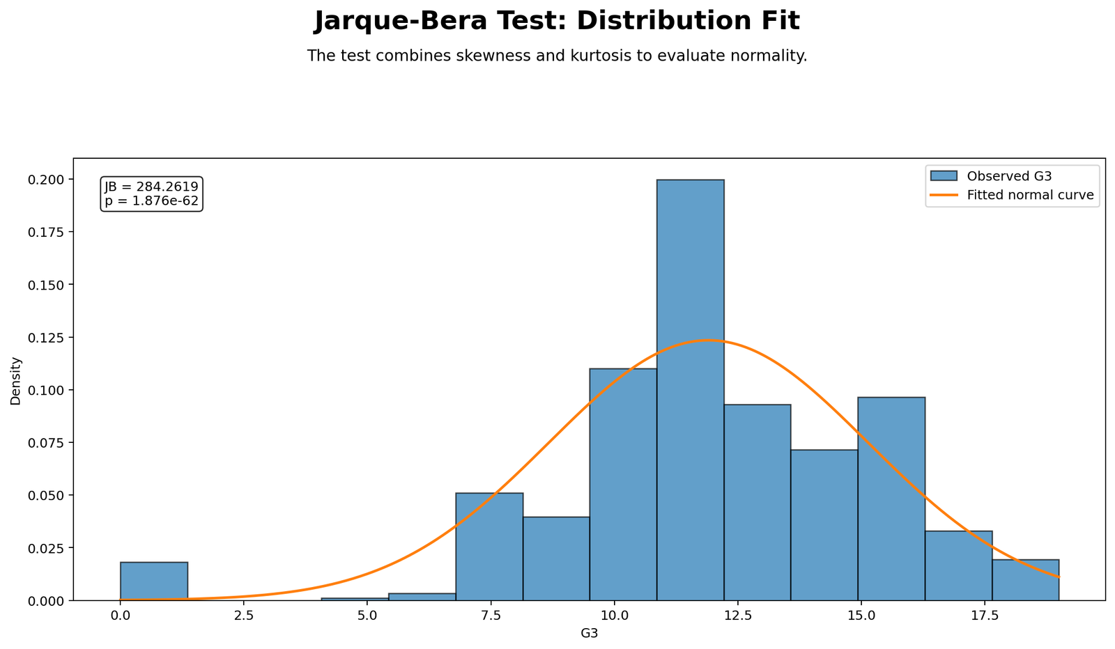
Detailed interpretation: This chart compares the empirical distribution of G3 with the normal distribution expected under the null hypothesis. The observed bars do not follow the fitted normal curve perfectly. The distribution is not a smooth symmetric bell shape, and the tail behavior is visibly different from normality.
Decision / reporting conclusion: The distribution-fit chart supports the formal Jarque Bera result. G3 should be reported as non-normal rather than normally distributed.
Python Chart 2: Normal Q-Q Plot
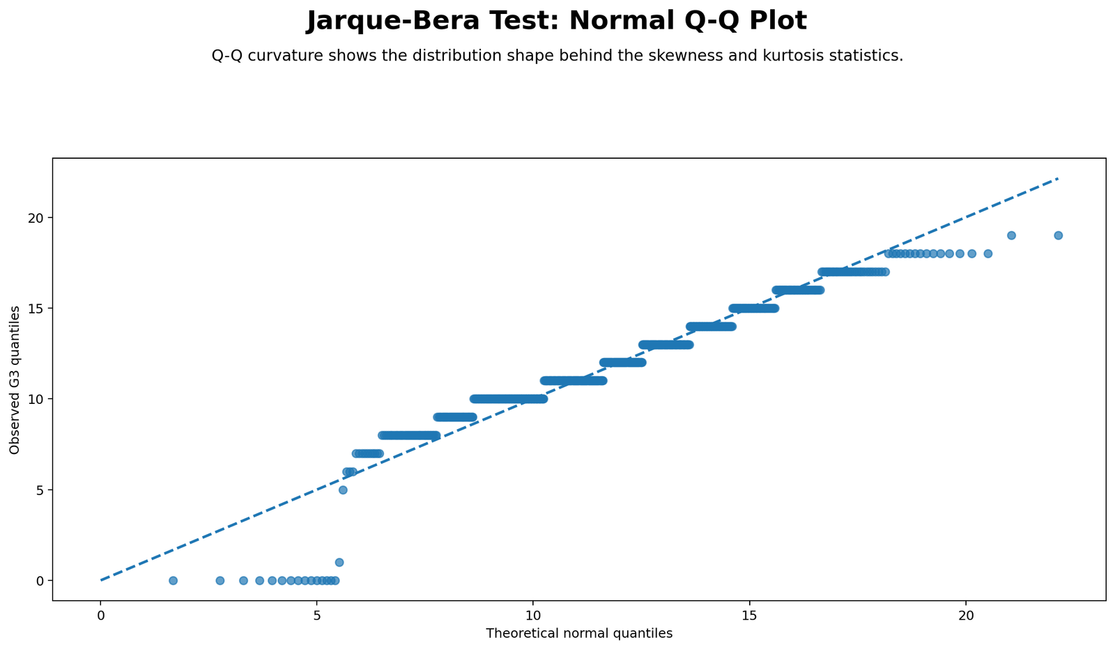
Detailed interpretation: In a normally distributed variable, the Q-Q plot points should stay close to the reference line. In this chart, the points depart from the line, especially in the tails. That departure confirms that the empirical quantiles of G3 do not match the expected normal quantiles.
Decision / reporting conclusion: The Q-Q plot supports rejection of normality. This chart should be interpreted together with the Q-Q plot normality check and the formal JB p-value.
Python Chart 3: Skewness and Kurtosis Contributions
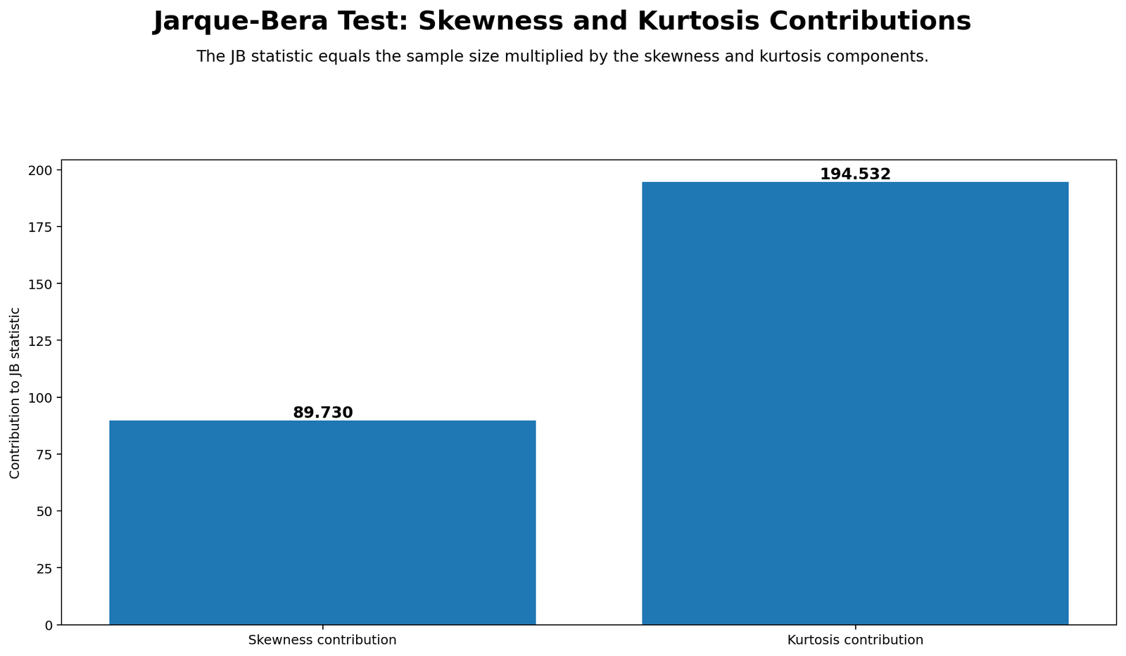
Detailed interpretation: This chart separates the two parts of the Jarque Bera formula. Skewness captures asymmetry, while kurtosis captures peak and tail behavior. The G3 variable has both negative skewness and elevated kurtosis, so the JB statistic is not inflated by only one minor issue. Both shape components help explain why normality is rejected.
Decision / reporting conclusion: The Jarque Bera rejection is shape-based. G3 differs from normality because of both asymmetry and abnormal tail/peak behavior.
Python Chart 4: Chi-Square Reference Curve
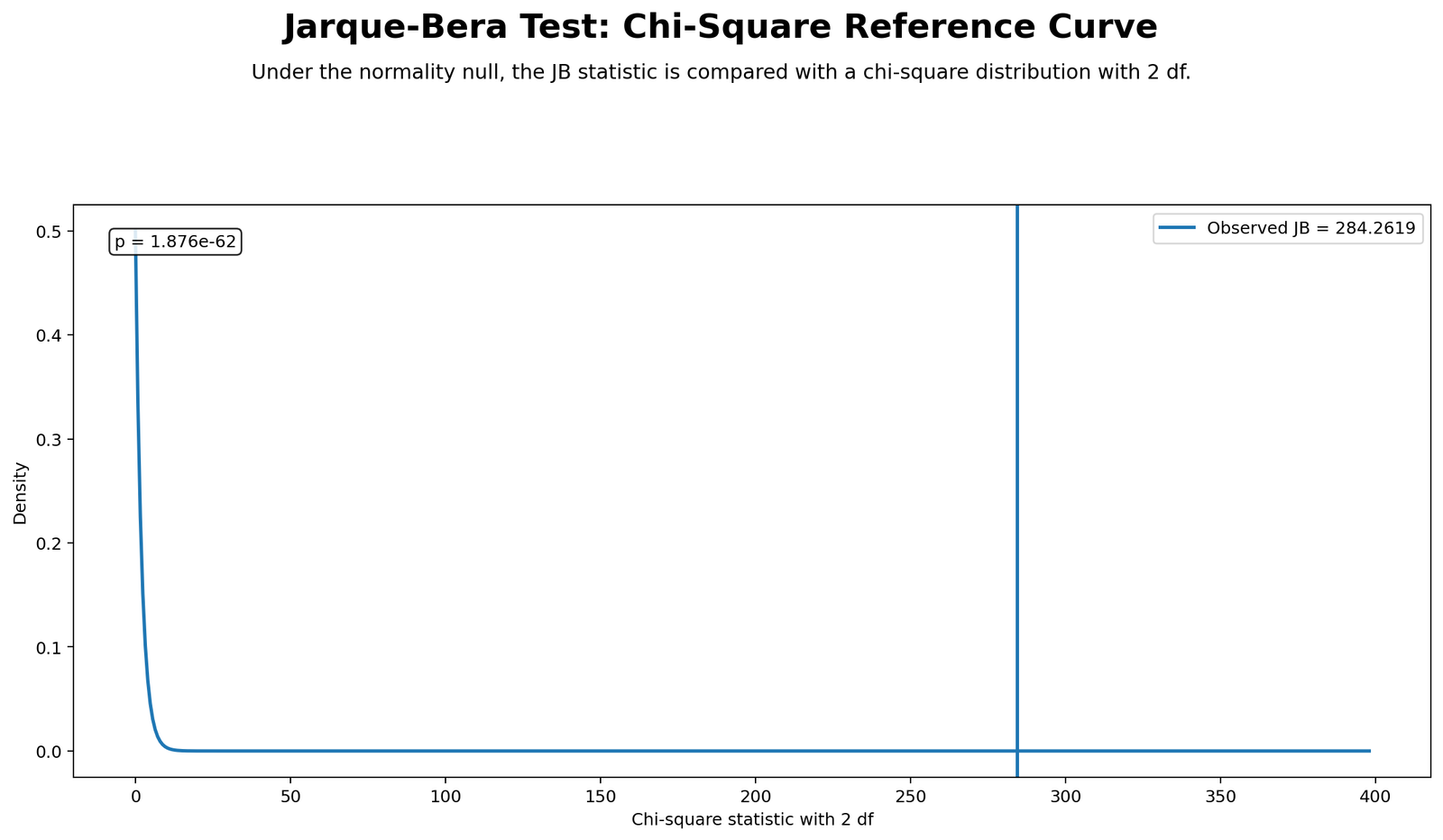
Detailed interpretation: Under normality, the JB statistic follows a chi-square distribution with 2 degrees of freedom. The observed statistic, about 284.26, is extremely far into the right tail of the reference distribution. This explains why the p-value is reported as essentially zero.
Decision / reporting conclusion: The observed statistic is far beyond the normal acceptance region. Reject the null hypothesis of normality for G3.
Python Chart 5: Jarque Bera Across Variables
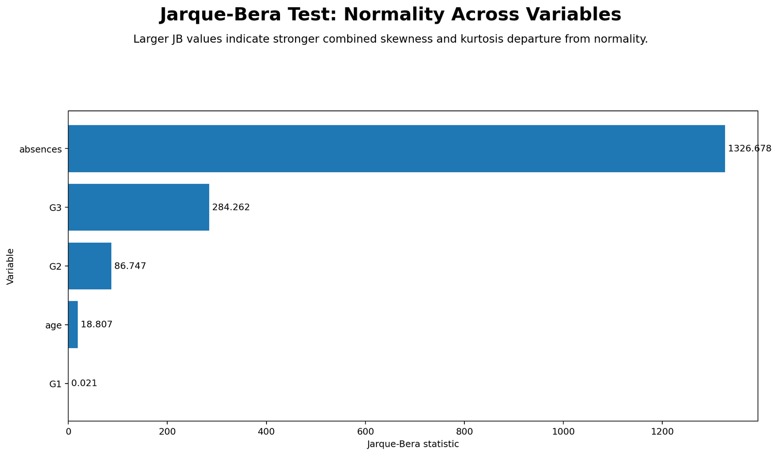
Detailed interpretation: This chart expands the analysis beyond G3. It helps identify which variables are closest to normality and which are most problematic. G1 is expected to be closer to normal than G3, while absences is expected to show stronger non-normality because count variables commonly have skewed distributions.
Decision / reporting conclusion: Jarque Bera can be used as a screening tool across several variables. G3 is clearly non-normal, and some variables may require additional checks, transformations, robust methods, or nonparametric alternatives.
Python Chart 6: Skewness-Kurtosis Map
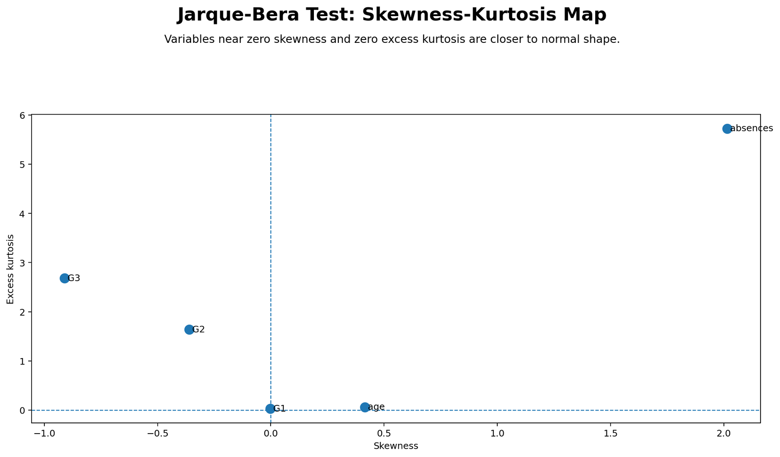
Detailed interpretation: The skewness-kurtosis map gives a two-dimensional view of normality. A variable close to skewness 0 and normal kurtosis is more normal-like. Variables far from that target have stronger shape problems. G3 sits away from the normal target because skewness and kurtosis are not ideal.
Decision / reporting conclusion: The map supports the formal Jarque Bera result by showing that G3 has a meaningful shape deviation from the normal benchmark.
Python Chart 7: Group Jarque Bera Comparison
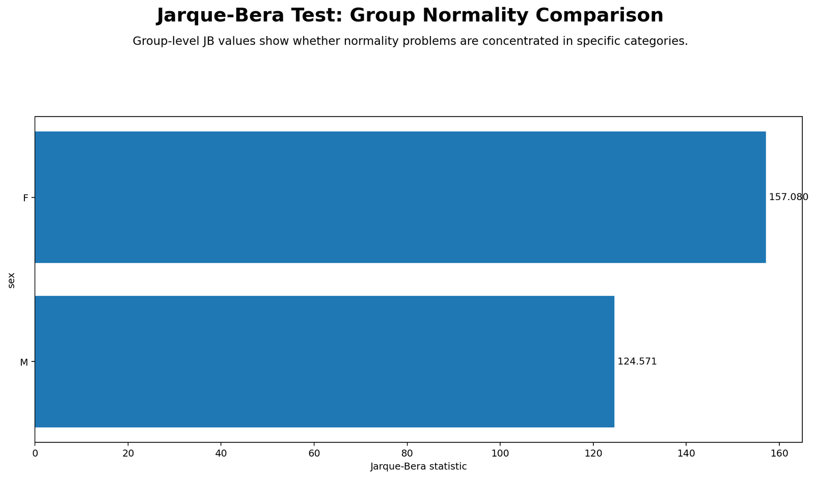
Detailed interpretation: This chart checks whether the normality issue disappears after splitting the data by sex group. The SPSS grouped results show that both female and male groups still reject normality. This means subgrouping alone does not solve the distribution problem.
Decision / reporting conclusion: G3 remains non-normal within groups. If group comparisons are performed later, normality and variance assumptions should be reported carefully.
R Chart-by-Chart Validation
The R charts validate the Python and SPSS findings using a separate statistical environment. This is important because matching results across SPSS, Python, and R make the final interpretation stronger and easier to defend in a report.
R Chart 1: Distribution Fit for Jarque Bera Test
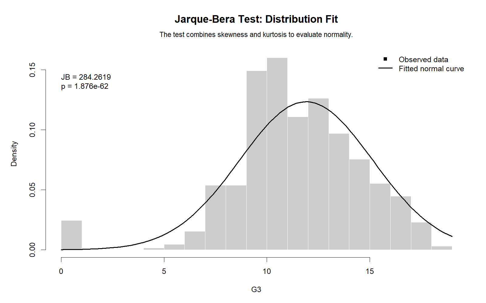
Detailed interpretation: The R distribution chart confirms the same pattern shown by Python. The G3 distribution does not follow the fitted normal curve exactly. The mismatch supports the conclusion that G3 has a shape problem relative to normality.
Decision / reporting conclusion: R validates the distribution-fit evidence that G3 is not normally distributed.
R Chart 2: Normal Q-Q Plot
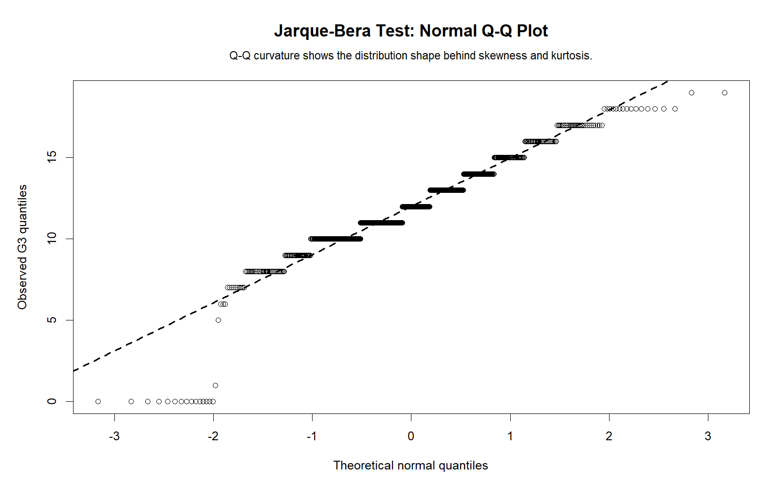
Detailed interpretation: The R Q-Q plot shows systematic departure from the normal reference line. The tails do not align perfectly with the theoretical normal distribution, which confirms that the empirical distribution of G3 is not normal.
Decision / reporting conclusion: The R Q-Q plot confirms the Python Q-Q interpretation and supports the Jarque Bera rejection.
R Chart 3: Skewness and Kurtosis Contributions
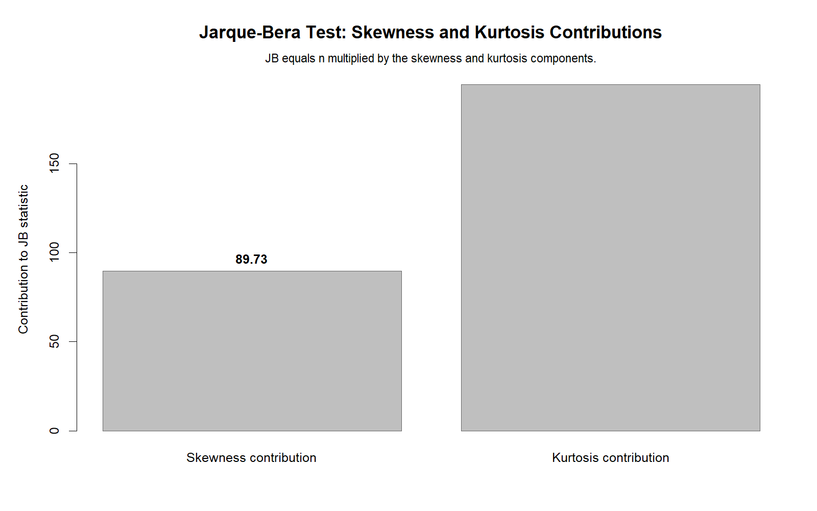
Detailed interpretation: The R contribution chart confirms that the significant Jarque Bera result comes from measurable distribution shape differences. Both skewness and kurtosis contribute to the final JB statistic.
Decision / reporting conclusion: R confirms that the normality violation is not only visual; it is mathematically reflected in the skewness and kurtosis components.
R Chart 4: Chi-Square Reference Curve
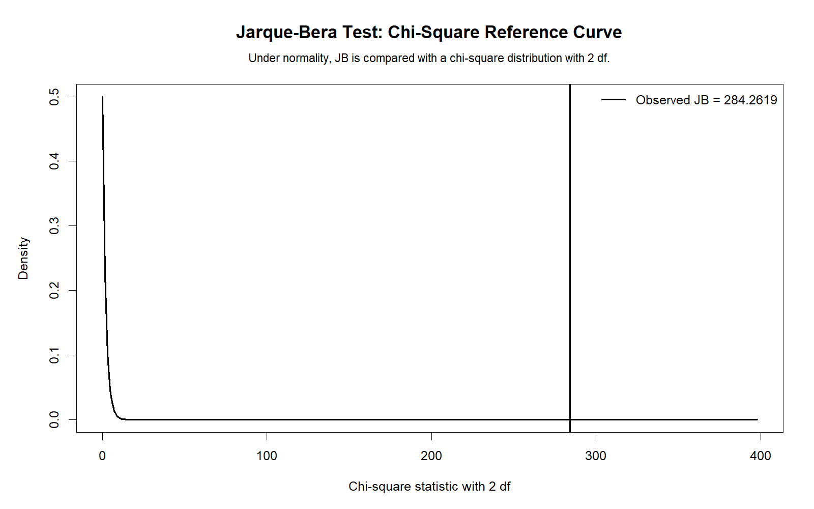
Detailed interpretation: The R reference curve shows that the observed JB statistic lies far in the right tail of the chi-square distribution. This makes the p-value extremely small and explains why the test rejects normality.
Decision / reporting conclusion: The R chi-square reference curve validates the SPSS p-value decision: reject normality for G3.
R Chart 5: Jarque Bera Across Variables
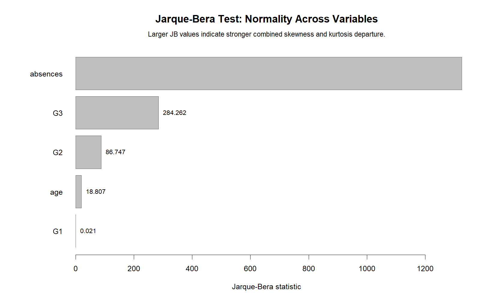
Detailed interpretation: This chart validates the Python comparison across variables. It helps identify which variables are most non-normal and which are closer to the normal distribution. Such comparison is helpful before choosing transformations, robust procedures, or model diagnostics.
Decision / reporting conclusion: R confirms that the Jarque Bera Test can be used as a multivariable screening method before deeper statistical modeling.
R Chart 6: Skewness-Kurtosis Map
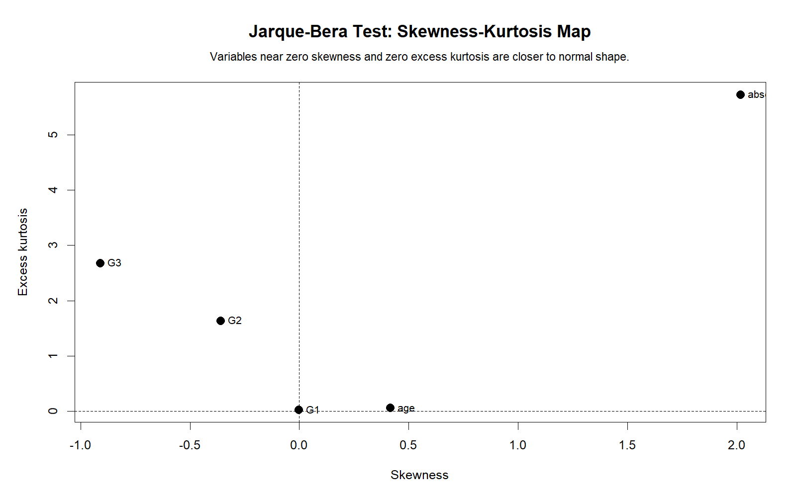
Detailed interpretation: The R map provides a compact visual summary of each variable’s skewness and kurtosis. Variables closer to the normality target are less problematic. Variables farther away require more careful assumption reporting.
Decision / reporting conclusion: R confirms that G3 does not sit close enough to the normality target to be reported as normally distributed.
R Chart 7: Group Jarque Bera Comparison
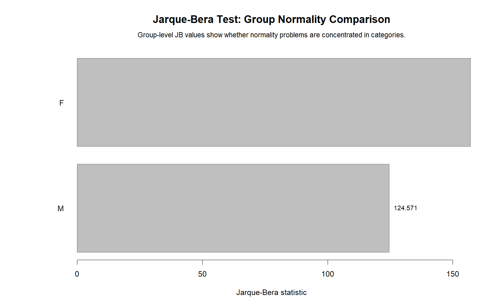
Detailed interpretation: The R grouped chart confirms the SPSS and Python group interpretation. Both groups show non-normality. The result indicates that normality violation is not only caused by mixing groups; it remains present inside the groups.
Decision / reporting conclusion: Group-wise R validation supports the final decision to reject normality for G3 in both overall and grouped contexts.
SPSS, Python, R and Excel Workflows for Jarque Bera Test
The Jarque Bera Test workflow is similar across software. The analyst should first inspect descriptive statistics, then calculate skewness and kurtosis, compute the JB statistic, calculate the chi-square p-value, inspect plots, and finally write the normality decision.
SPSS Workflow
| Step | SPSS Menu or Syntax | Purpose |
|---|---|---|
| Open dataset | File > Open > Data | Load the SPSS-ready dataset. |
| Inspect variable | Analyze > Descriptive Statistics > Explore | Generate descriptives, histogram, Q-Q plot and normality tests. |
| Record shape values | Descriptives table | Use skewness and kurtosis for JB interpretation. |
| Compute JB statistic | Transform > Compute Variable or syntax | Apply the Jarque Bera formula. |
| Compute p-value | Chi-square CDF | Compare JB to chi-square distribution with 2 df. |
| Export output | OUTPUT EXPORT | Save the SPSS output PDF for WordPress resources. |
Python Workflow
| Step | Python Action | Purpose |
|---|---|---|
| Read data | pandas.read_csv() | Load the dataset. |
| Select target variable | df["G3"].dropna() | Prepare valid values. |
| Run Jarque Bera | scipy.stats.jarque_bera() | Get JB statistic and p-value. |
| Calculate shape | skew() and kurtosis() | Explain why normality is rejected. |
| Create charts | matplotlib, scipy and statsmodels | Create histogram, Q-Q plot and reference curve. |
| Report decision | APA sentence | Write result clearly for readers. |
R Workflow
| Step | R Action | Purpose |
|---|---|---|
| Read data | read.csv() or readr::read_csv() | Load the dataset. |
| Select variable | na.omit(df$G3) | Remove missing values. |
| Run JB test | tseries::jarque.bera.test() | Calculate statistic and p-value. |
| Calculate shape | moments::skewness() and moments::kurtosis() | Explain skewness and kurtosis. |
| Create validation charts | ggplot2 or base R | Validate Python and SPSS results visually. |
| Write report | APA wording | Summarize JB statistic, p-value and conclusion. |
Excel Workflow
| Excel Task | Formula or Tool | Purpose |
|---|---|---|
| Count cases | =COUNT(A2:A650) | Calculate sample size. |
| Calculate skewness | =SKEW(A2:A650) | Measure asymmetry. |
| Calculate excess kurtosis | =KURT(A2:A650) | Measure tail/peak departure. |
| Compute JB statistic | =(COUNT(A2:A650)/6)*(SKEW(A2:A650)^2+(KURT(A2:A650)^2/4)) | Apply the JB formula using Excel’s excess kurtosis. |
| Compute p-value | =CHISQ.DIST.RT(B10,2) | Calculate chi-square right-tail probability. |
| Make histogram | Insert > Statistic Chart > Histogram | Visually inspect distribution shape. |
If the Jarque Bera Test is part of a regression or model-checking workflow, use it with other model diagnostics. For functional form problems, see the Ramsey RESET test. For variance problems, see the Goldfeld-Quandt test. For repeated-measures analysis, assumption checks may also involve Mauchly’s test of sphericity and the Greenhouse-Geisser correction.
Code Blocks for Jarque Bera Test
SPSS Syntax for Jarque Bera Test
* Jarque Bera Test in SPSS.
* Main target variable: G3.

TITLE "Jarque Bera Test: G3 final grade normality check".

GET FILE='D:\DATA ANALYSIS\B Normality and Assumption Tests\Jarque Bera Test\SPSS_Output\sav\Jarque-Bera-Test-data.sav'.

EXAMINE VARIABLES=G3
  /PLOT BOXPLOT HISTOGRAM NPPLOT
  /COMPARE GROUPS
  /STATISTICS DESCRIPTIVES
  /CINTERVAL 95
  /MISSING LISTWISE
  /NOTOTAL.

EXAMINE VARIABLES=G3 BY sex
  /PLOT BOXPLOT HISTOGRAM NPPLOT
  /COMPARE GROUPS
  /STATISTICS DESCRIPTIVES
  /CINTERVAL 95
  /MISSING LISTWISE
  /NOTOTAL.

* Verified values from SPSS custom calculation output.
DATASET DECLARE JB_Calculation.
DATASET ACTIVATE JB_Calculation.

INPUT PROGRAM.
NUMERIC jb_n_calc jb_skewness jb_kurtosis jb_excess_kurtosis jb_skew_component jb_kurt_component jarque_bera jb_p_value jb_reject_05.
END CASE.
END FILE.
END INPUT PROGRAM.

COMPUTE jb_n_calc = 649.
COMPUTE jb_skewness = -0.91080.
COMPUTE jb_kurtosis = 5.68212.
COMPUTE jb_excess_kurtosis = jb_kurtosis - 3.
COMPUTE jb_skew_component = jb_skewness**2.
COMPUTE jb_kurt_component = (jb_excess_kurtosis**2) / 4.
COMPUTE jarque_bera = (jb_n_calc / 6) * (jb_skew_component + jb_kurt_component).
COMPUTE jb_p_value = 1 - CDF.CHISQ(jarque_bera,2).
COMPUTE jb_reject_05 = (jb_p_value < .05).
EXECUTE.

FORMATS jb_n_calc (F8.0)
  jb_skewness jb_kurtosis jb_excess_kurtosis jb_skew_component jb_kurt_component jarque_bera jb_p_value (F12.5)
  jb_reject_05 (F4.0).

LIST jb_n_calc jb_skewness jb_kurtosis jb_excess_kurtosis jb_skew_component jb_kurt_component jarque_bera jb_p_value jb_reject_05.

OUTPUT SAVE OUTFILE='D:\DATA ANALYSIS\B Normality and Assumption Tests\Jarque Bera Test\SPSS_Output\spv\Jarque-Bera-Test-output.spv'.

OUTPUT EXPORT
  /CONTENTS EXPORT=VISIBLE LAYERS=PRINTSETTING MODELVIEWS=PRINTSETTING
  /PDF DOCUMENTFILE='D:\DATA ANALYSIS\B Normality and Assumption Tests\Jarque Bera Test\SPSS_Output\pdf\Jarque-Bera-Test-SPSS-Output.pdf'.
Python Code for Jarque Bera Test
import pandas as pd
import numpy as np
import matplotlib.pyplot as plt
from scipy import stats
from scipy.stats import jarque_bera, skew, kurtosis, chi2, norm
import statsmodels.api as sm

# Load data
df = pd.read_csv("dataset.csv")

# Target variable
x = pd.to_numeric(df["G3"], errors="coerce").dropna()
n = len(x)

# Jarque Bera Test
jb_stat, jb_p = jarque_bera(x)

# Shape statistics
sk = skew(x, bias=False)
excess_kurt = kurtosis(x, fisher=True, bias=False)
ordinary_kurt = excess_kurt + 3

print("N:", n)
print("Skewness:", sk)
print("Excess Kurtosis:", excess_kurt)
print("Ordinary Kurtosis:", ordinary_kurt)
print("Jarque Bera Statistic:", jb_stat)
print("p-value:", jb_p)

alpha = 0.05
if jb_p < alpha:
    print("Reject H0: G3 is not normally distributed.")
else:
    print("Fail to reject H0: no significant evidence against normality.")

# Distribution fit chart
mu = x.mean()
sd = x.std(ddof=1)
xx = np.linspace(x.min(), x.max(), 400)

plt.figure(figsize=(10, 6))
plt.hist(x, bins=20, density=True, alpha=0.70, edgecolor="white")
plt.plot(xx, norm.pdf(xx, mu, sd), linewidth=2)
plt.title("Jarque Bera Test: Distribution Fit for G3")
plt.xlabel("G3 final grade")
plt.ylabel("Density")
plt.tight_layout()
plt.show()

# Q-Q plot
sm.qqplot(x, line="s")
plt.title("Normal Q-Q Plot for G3")
plt.tight_layout()
plt.show()

# Chi-square reference curve
x_chi = np.linspace(0, 20, 400)
plt.figure(figsize=(10, 6))
plt.plot(x_chi, chi2.pdf(x_chi, df=2), linewidth=2)
plt.axvline(jb_stat, linestyle="--")
plt.title("Jarque Bera Statistic on Chi-Square Reference Curve")
plt.xlabel("Chi-square value")
plt.ylabel("Density")
plt.tight_layout()
plt.show()

# Across variables
vars_to_check = ["G1", "G2", "G3", "age", "absences"]
rows = []

for col in vars_to_check:
    y = pd.to_numeric(df[col], errors="coerce").dropna()
    stat, p = jarque_bera(y)
    rows.append({
        "variable": col,
        "N": len(y),
        "skewness": skew(y, bias=False),
        "ordinary_kurtosis": kurtosis(y, fisher=False, bias=False),
        "JB": stat,
        "p_value": p,
        "reject_05": p < 0.05
    })

summary = pd.DataFrame(rows)
print(summary)

# Group comparison by sex
group_rows = []
for group, sub in df.groupby("sex"):
    y = pd.to_numeric(sub["G3"], errors="coerce").dropna()
    stat, p = jarque_bera(y)
    group_rows.append({
        "sex": group,
        "N": len(y),
        "mean": y.mean(),
        "sd": y.std(ddof=1),
        "skewness": skew(y, bias=False),
        "ordinary_kurtosis": kurtosis(y, fisher=False, bias=False),
        "JB": stat,
        "p_value": p,
        "reject_05": p < 0.05
    })

group_summary = pd.DataFrame(group_rows)
print(group_summary)
R Code for Jarque Bera Test
library(readr)
library(dplyr)
library(ggplot2)
library(tseries)
library(moments)

# Load data
df <- read_csv("dataset.csv")

# Target variable
x <- na.omit(as.numeric(df$G3))

# Jarque Bera Test
jb_result <- jarque.bera.test(x)
print(jb_result)

# Shape statistics
n <- length(x)
sk <- skewness(x)
ordinary_kurt <- kurtosis(x)
excess_kurt <- ordinary_kurt - 3

cat("N:", n, "\n")
cat("Skewness:", sk, "\n")
cat("Ordinary Kurtosis:", ordinary_kurt, "\n")
cat("Excess Kurtosis:", excess_kurt, "\n")

if(jb_result$p.value < 0.05){
  cat("Reject H0: G3 is not normally distributed.\n")
} else {
  cat("Fail to reject H0: no significant evidence against normality.\n")
}

# Distribution fit
ggplot(data.frame(G3=x), aes(x=G3)) +
  geom_histogram(aes(y=after_stat(density)), bins=20, fill="skyblue", color="white") +
  stat_function(fun=dnorm, args=list(mean=mean(x), sd=sd(x)), linewidth=1.2) +
  labs(title="Jarque Bera Test: Distribution Fit for G3",
       x="G3 final grade",
       y="Density")

# Q-Q plot
ggplot(data.frame(sample=x), aes(sample=sample)) +
  stat_qq() +
  stat_qq_line() +
  labs(title="Normal Q-Q Plot for G3")

# Across variables
vars_to_check <- c("G1", "G2", "G3", "age", "absences")

summary_tbl <- lapply(vars_to_check, function(v){
  y <- na.omit(as.numeric(df[[v]]))
  jb <- jarque.bera.test(y)
  data.frame(
    variable = v,
    N = length(y),
    skewness = skewness(y),
    ordinary_kurtosis = kurtosis(y),
    JB = as.numeric(jb$statistic),
    p_value = jb$p.value,
    reject_05 = jb$p.value < 0.05
  )
}) |> bind_rows()

print(summary_tbl)

# Group comparison by sex
group_tbl <- df |>
  group_by(sex) |>
  summarise(
    N = sum(!is.na(G3)),
    mean = mean(G3, na.rm=TRUE),
    sd = sd(G3, na.rm=TRUE),
    skewness = skewness(na.omit(G3)),
    ordinary_kurtosis = kurtosis(na.omit(G3)),
    JB = as.numeric(jarque.bera.test(na.omit(G3))$statistic),
    p_value = jarque.bera.test(na.omit(G3))$p.value,
    reject_05 = p_value < 0.05,
    .groups = "drop"
  )

print(group_tbl)
Excel Formulas for Jarque Bera Test
Assume G3 values are in A2:A650.

Sample size:
=COUNT(A2:A650)

Mean:
=AVERAGE(A2:A650)

Standard deviation:
=STDEV.S(A2:A650)

Skewness:
=SKEW(A2:A650)

Excess kurtosis:
=KURT(A2:A650)

Ordinary kurtosis:
=KURT(A2:A650)+3

Jarque Bera statistic:
=(COUNT(A2:A650)/6)*(SKEW(A2:A650)^2+(KURT(A2:A650)^2/4))

If the JB statistic is in B10, p-value:
=CHISQ.DIST.RT(B10,2)

Decision:
=IF(B11<0.05,"Reject normality","Fail to reject normality")

Interpretation:
If p-value < .05, the variable significantly departs from normality.
If p-value >= .05, there is no significant Jarque Bera evidence against normality.
APA Reporting Wording for Jarque Bera Test
When reporting the Jarque Bera Test, include the variable name, sample size, JB statistic, p-value, skewness, kurtosis, and final normality decision. Do not only write “the data were not normal.” Explain what feature of the distribution created the result.
APA-Style Jarque Bera Test Report
A Jarque Bera Test was conducted to assess whether final grades (G3) followed a normal distribution. The test was statistically significant, JB = 284.26, p < .001, N = 649, indicating that G3 significantly departed from normality. The distribution showed negative skewness, skewness = -.91, and elevated kurtosis, excess kurtosis approximately 2.68 to 2.71 depending on estimator. Therefore, the normality assumption was not supported.
Short Report Sentence
The Jarque Bera Test rejected normality for G3, JB = 284.26, p < .001, showing that the final-grade distribution was significantly non-normal because of skewness and kurtosis departures.
Student-Friendly Report Example
The G3 final-grade values do not form a normal bell-shaped distribution. The Jarque Bera Test found a very large statistic and a p-value below .001, so the normality assumption should be rejected.
If this normality check is reported before a hypothesis test, also report the practical result of the main analysis. For example, a confidence interval can make the result easier to understand, and an effect size can show the size of a difference beyond the p-value.
Common Mistakes in Jarque Bera Test Interpretation
| Mistake | Why It Is a Problem | Correct Practice |
|---|---|---|
| Confusing ordinary kurtosis and excess kurtosis | Some formulas use ordinary kurtosis, while software often reports excess kurtosis. | Check the software definition before calculating JB. |
| Reporting only the p-value | The reader does not know whether skewness or kurtosis caused the result. | Report JB statistic, p-value, skewness and kurtosis. |
| Ignoring plots | A p-value does not show the shape of the distribution. | Use histograms, Q-Q plots and P-P plots with the test. |
| Assuming non-normal data are unusable | Many methods are robust, especially with large samples. | Consider the research design, model residuals, sample size and robustness. |
| Testing the wrong object | In regression, residual normality is often more important than raw-variable normality. | Check model residuals when the method requires residual normality. |
| Using one normality test only | Different tests detect different types of non-normality. | Compare JB with Shapiro-Wilk, K-S, Lilliefors, Ryan-Joiner, D’Agostino-Pearson and visual plots. |
Key reminder: The Jarque Bera Test tells you whether skewness and kurtosis are consistent with normality. It does not automatically choose the final statistical method for you. Your final method should depend on the research question, sample size, variable type, assumptions, and reporting purpose.
When to Use Jarque Bera Test
Use the Jarque Bera Test when you want a formal normality test based directly on skewness and kurtosis. It is commonly used in economics, finance, education, social science, business analytics and general statistical reporting.
| Use Case | Why Jarque Bera Helps | Example from This Guide |
|---|---|---|
| Testing normality of a continuous variable | Combines skewness and kurtosis into one statistic. | G3 final grade was tested. |
| Explaining why normality fails | Shows whether asymmetry or tail behavior is the issue. | G3 has negative skewness and high kurtosis. |
| Comparing variables | JB can screen multiple variables before modeling. | G1, G2, G3, age and absences were compared. |
| Checking groups | Normality can be evaluated within subgroups. | G3 was checked by sex group. |
| Preparing for later tests | Assumption diagnostics guide method choice. | Normality was rejected before selecting follow-up methods. |
If non-normality is caused by strong skewness, a transformation may sometimes help. For example, the reciprocal transformation may be useful for some right-skewed variables, but it should be justified with before-and-after evidence. If the issue is variance homogeneity rather than normality, check Levene test, Brown-Forsythe test, or Cochran C test.
In model-based research, the Jarque Bera Test can be part of a larger diagnostic workflow. For example, the Ramsey RESET test checks model specification, while the Goldfeld-Quandt test checks heteroscedasticity. For repeated-measures designs, see Mauchly’s test of sphericity and the Greenhouse-Geisser correction. For applied R workflows, the clinical trial data analysis using R guide shows how diagnostics connect with real reporting.
Downloads and Resources for Jarque Bera Test
The resources below include the SPSS output PDF, Python charts, and R validation charts used in this Jarque Bera Test guide.
Download SPSS Output PDF
Verified SPSS output for G3 descriptives, normality tests, grouped normality context and Jarque Bera calculation.
Copy Jarque Bera Test Code
Use the SPSS, Python, R and Excel code blocks to reproduce the Jarque Bera workflow.
Python Chart 1: Distribution Fit
Histogram and fitted normal curve for the G3 final-grade variable.
R Chart 1: Distribution Fit
R validation chart showing the same distribution-fit interpretation.
FAQs About Jarque Bera Test
What is the Jarque Bera Test?
The Jarque Bera Test is a normality test that checks whether a variable has skewness close to 0 and ordinary kurtosis close to 3, which are expected under a normal distribution.
What are the null and alternative hypotheses of the Jarque Bera Test?
The null hypothesis says the data follow a normal distribution. The alternative hypothesis says the data do not follow a normal distribution.
How do I interpret a significant Jarque Bera Test?
A significant result means the variable significantly departs from normality. You should inspect skewness, kurtosis, histograms, Q-Q plots and the purpose of the analysis before choosing the next method.
What was the Jarque Bera result for G3 in this guide?
The verified Jarque Bera result for G3 was JB = 284.26194 with p = 0.00000. Therefore, normality was rejected.
Is Jarque Bera the same as Shapiro-Wilk?
No. Both are normality tests, but Jarque Bera is based on skewness and kurtosis. Shapiro-Wilk uses a different normality-testing logic.
Can Jarque Bera Test be calculated in SPSS?
Yes. SPSS does not always provide a direct menu option for Jarque Bera, but it can be calculated using syntax from sample size, skewness and kurtosis.
Can Jarque Bera Test be calculated in Excel?
Yes. Use COUNT, SKEW, KURT and CHISQ.DIST.RT. Excel’s KURT function returns excess kurtosis, so it can be used directly in the common Excel formula.
What should I do if the Jarque Bera Test rejects normality?
Check plots, look for outliers, consider transformations, evaluate residuals if using regression, use robust procedures if appropriate, or choose nonparametric methods depending on the research question.
Final Conclusion
The Jarque Bera Test is a useful normality test because it links the formal p-value directly to skewness and kurtosis. In this Salar Cafe example, the verified SPSS calculation gives Jarque Bera = 284.26194 and p = 0.00000 for the G3 final-grade variable. Therefore, the null hypothesis of normality is rejected.
The Python charts and R validation charts support the same interpretation. The distribution fit chart shows mismatch with the normal curve, the Q-Q plot shows tail deviations, the skewness-kurtosis contribution charts explain why the statistic is large, and the chi-square reference curve shows why the p-value is extremely small. Grouped analysis also shows that non-normality remains present within sex groups.
The correct reporting conclusion is not simply “the data are bad.” The correct conclusion is that G3 is statistically non-normal because it has meaningful skewness and kurtosis departures. Any later analysis should consider the research design, sample size, robustness of the method, distribution plots, and relevant assumption checks.

