
Goodness-of-Fit, Normality Testing, Empirical CDF and W2 Statistic
Cramer von Mises Test: Formula, Interpretation, SPSS, Python, R and Excel Guide
Cramer von Mises Test is a goodness-of-fit test that compares the empirical cumulative distribution function of the sample with a theoretical distribution such as the normal distribution. It uses the squared distance between the empirical CDF and the fitted CDF across the whole distribution. This Salar Cafe guide explains the Cramer von Mises Test with verified SPSS output, Python charts, R validation charts, formula, W2 statistic, Monte Carlo p-value, Excel workflow, APA reporting, common mistakes and downloadable resources.
Quick Answer: Cramer von Mises Test Result
The verified Cramer von Mises Test result for the main variable G3 final grade shows N = 649, mean = 11.9060, standard deviation = 3.2307, W2 = 1.1241, and Monte Carlo p ≈ 0.00002. Because the p-value is far below .05, the normality null hypothesis is rejected. This means the G3 distribution does not follow the fitted normal distribution closely enough under the Cramer von Mises goodness-of-fit criterion.
Hypothesis-style interpretation: The null hypothesis says that the sample follows the fitted normal distribution. The alternative hypothesis says that the sample does not follow the fitted normal distribution. Since p ≈ 0.00002, the decision is to reject H0. The Cramer von Mises Test therefore provides strong evidence that the G3 final grade distribution departs from normality.
Final interpretation: The Cramer von Mises Test indicates that the G3 final grade variable is not normally distributed. The empirical CDF differs enough from the fitted normal CDF to produce a statistically significant W2 statistic. In practical reporting, say that the data show a significant departure from normality and support the conclusion with the distribution chart, empirical CDF plot, Q-Q plot, squared CDF gap chart and Monte Carlo reference distribution.
Important note: A significant Cramer von Mises Test does not automatically mean the analysis is invalid. In large samples, normality tests can detect small departures. Always combine the p-value with visual checks, sample size, skewness, kurtosis, Q-Q plots, research purpose and the robustness of the planned method.
Table of Contents
- What Is the Cramer von Mises Test?
- Why the Cramer von Mises Test Matters
- Cramer von Mises Test Formula
- Null and Alternative Hypothesis
- Dataset and Variables Used
- Verified SPSS Output Interpretation
- Python Chart-by-Chart Interpretation
- R Chart-by-Chart Validation
- SPSS, R, Python and Excel Workflows
- Code Blocks for Cramer von Mises Test
- APA Reporting Wording
- Common Mistakes
- When to Use the Cramer von Mises Test
- Downloads and Resources
- Related Guides
- FAQs
What Is the Cramer von Mises Test?
The Cramer von Mises Test is a goodness-of-fit test used to compare a sample distribution with a theoretical distribution. In many applied statistics tasks, it is used as a normality test. The test checks whether the empirical cumulative distribution function, also called the empirical CDF, stays close to the fitted theoretical CDF across the full range of observed values.
The Cramer von Mises Test is based on squared differences. This means it does not focus only on the largest single distance. Instead, it accumulates the squared gaps between the empirical distribution and the theoretical distribution. If these gaps are small across the distribution, the W2 statistic is small. If the gaps are large or spread across the distribution, W2 becomes larger and the p-value becomes smaller.
This makes the test different from the Kolmogorov-Smirnov test, which focuses on the maximum distance between the empirical CDF and theoretical CDF. It is also related to other normality and goodness-of-fit tools such as the D’Agostino-Pearson test, Lilliefors test, Ryan-Joiner test, Q-Q plot normality check, Q-Q plot normality check 2, and P-P plot normality check.
Practical meaning: The Cramer von Mises Test asks whether the whole observed distribution is close enough to the fitted theoretical distribution. It is especially useful when you want a distribution-wide goodness-of-fit decision rather than only a visual impression.
Why the Cramer von Mises Test Matters
The Cramer von Mises Test matters because many statistical methods assume that a variable, residual, or model error distribution is approximately normal. When the assumption is not reasonable, test results, confidence intervals, p-values and model interpretation may become less reliable. The Cramer von Mises Test provides a formal way to compare the observed distribution with the fitted normal distribution.
In the worked example, the main variable is G3 final grade. The Cramer von Mises statistic is W2 = 1.1241, and the Monte Carlo p-value is approximately 0.00002. This is very strong evidence that the empirical distribution of G3 does not match the fitted normal distribution. The charts then show where and how the distribution departs from normality.
| Reason to Use the Test | What It Checks | Why It Helps |
|---|---|---|
| Normality evaluation | Compares empirical CDF with fitted normal CDF. | Gives a formal p-value for normality evidence. |
| Distribution-wide comparison | Uses squared gaps across the whole CDF. | Does not rely only on one maximum distance. |
| Visual confirmation | Can be paired with Q-Q plots, histograms and CDF charts. | Helps explain why the test is significant. |
| Model assumption checking | Useful for checking variables or residuals. | Supports decisions before t-tests, ANOVA, regression or reporting. |
| Monte Carlo support | Reference distribution can be simulated. | Useful when exact p-values are not directly available in SPSS. |
For a broader assumption-checking workflow, use the Cramer von Mises Test with descriptive and graphical tools such as descriptive statistics, frequency distribution, histogram interpretation, box plot interpretation, five-number summary, and coefficient of variation.
Cramer von Mises Test Formula
The Cramer von Mises Test compares the empirical CDF with the fitted theoretical CDF. If the observations are sorted from smallest to largest as x(1), x(2), …, x(n), and F(x) is the fitted theoretical CDF, the common one-sample statistic is:
In this formula, n is the sample size, F(x(i)) is the fitted theoretical CDF value for the ordered observation, and (2i − 1)/(2n) is the expected empirical plotting position. The statistic becomes larger when the fitted CDF and empirical CDF are far apart.
How to Interpret W2
| Component | Meaning | Interpretation |
|---|---|---|
| Small W2 | Empirical CDF is close to theoretical CDF. | Data are more consistent with the fitted distribution. |
| Large W2 | Empirical CDF is far from theoretical CDF across the distribution. | Data depart from the fitted distribution. |
| Small p-value | Observed W2 is unlikely under the null distribution. | Reject the goodness-of-fit null hypothesis. |
| Large p-value | Observed W2 is plausible under the null distribution. | Do not reject the fitted distribution assumption. |
Formula caution: If the mean and standard deviation are estimated from the sample, the reference distribution differs from a fully specified distribution test. This is why Monte Carlo simulation is often useful for practical p-value estimation.
Null and Alternative Hypothesis for the Cramer von Mises Test
The Cramer von Mises Test is a formal goodness-of-fit test. In this post, it is used as a normality test for the G3 final grade variable.
| Hypothesis | Statement | Meaning in This Example |
|---|---|---|
| Null hypothesis | H0: The sample follows the fitted normal distribution. | The G3 final grade distribution is consistent with normality. |
| Alternative hypothesis | H1: The sample does not follow the fitted normal distribution. | The G3 final grade distribution departs from normality. |
| Decision rule | Reject H0 if p < .05. | If the p-value is below .05, normality is rejected. |
| Observed result | W2 = 1.1241, Monte Carlo p ≈ 0.00002. | The p-value is much smaller than .05. |
Hypothesis decision: Because p ≈ 0.00002 is less than .05, reject the null hypothesis. The G3 final grade variable does not follow the fitted normal distribution according to the Cramer von Mises Test.
Interpretation nuance: In a large sample such as N = 649, a formal normality test can detect departures that may not be severe enough to invalidate every analysis. Use the test result together with the Q-Q plot, histogram, empirical CDF plot, sample size and planned statistical method.
Dataset and Variables Used
The worked example uses a student performance-style dataset. The main tested variable is G3 final grade, which is a numeric outcome variable. The Cramer von Mises Test evaluates whether the observed G3 distribution follows a fitted normal distribution based on the sample mean and standard deviation.
| Variable | Role | Verified Value / Use | Why It Matters |
|---|---|---|---|
| G3 | Main tested variable | N = 649, mean = 11.9060, SD = 3.2307 | Used to test whether final grades follow a fitted normal distribution. |
| G1 | Comparison variable | Can be included in W2 across variables chart. | Shows whether earlier grades have stronger or weaker distribution departures. |
| G2 | Comparison variable | Can be compared against G3. | Useful for identifying which grade variable is closest to normal. |
| absences | Count variable | Usually non-normal and right-skewed. | Often shows larger departures in distribution tests. |
| studytime / sex / school | Grouping or comparison variables | Used for group W2 comparison where relevant. | Helps compare normality behavior across groups. |
Before interpreting a formal normality result, it is useful to summarize the data with descriptive statistics, frequency distribution, histogram interpretation, and five-number summary. If the variable has extreme values, also review box plot interpretation.
Verified SPSS Output Interpretation
The verified SPSS output supports the Cramer von Mises Test interpretation for the G3 final grade variable. Because SPSS does not always provide a direct one-click Cramer von Mises normality workflow in the same way it provides common descriptive output, the analysis can be supported by computed empirical CDF values, fitted normal CDF values, squared gap contributions and Monte Carlo reference simulation.
The SPSS output PDF for this guide is available here:
Download SPSS Cramer von Mises Output PDF
Verified SPSS output for Cramer von Mises Test, W2 statistic, normality interpretation and reporting support.
Copy SPSS, Python, R and Excel Code
Use the code section below to reproduce the Cramer von Mises Test workflow.
SPSS Result Summary
| SPSS Output Item | Verified Result | Interpretation |
|---|---|---|
| Tested variable | G3 final grade | The outcome variable checked against a fitted normal distribution. |
| Valid N | 649 | The test is based on 649 observations. |
| Mean | 11.9060 | The fitted normal distribution uses the sample location. |
| Standard deviation | 3.2307 | The fitted normal distribution uses the sample spread. |
| Cramer von Mises statistic | W2 = 1.1241 | The empirical CDF differs from the fitted normal CDF enough to produce a large statistic. |
| Monte Carlo p-value | ≈ 0.00002 | The result is statistically significant and normality is rejected. |
| Decision at α = .05 | Reject H0 | G3 does not follow the fitted normal distribution. |
SPSS Decision Summary
SPSS interpretation summary: The Cramer von Mises Test for G3 produced W2 = 1.1241 with Monte Carlo p ≈ 0.00002. Since the p-value is below .05, reject the null hypothesis of normality. The G3 final grade distribution shows a statistically significant departure from the fitted normal distribution. The SPSS result should be interpreted together with the distribution fit chart, empirical CDF chart, Q-Q plot and squared CDF gap chart.
How This SPSS Output Relates to Other Normality Tests
The Cramer von Mises Test is one part of a larger normality-checking toolkit. If you want to compare results, use the Kolmogorov-Smirnov test, Lilliefors test, D’Agostino-Pearson test, and Ryan-Joiner test. If your analysis later uses regression, also examine residual diagnostics and model form using the Ramsey RESET test.
Python Chart-by-Chart Interpretation
The Python charts show the Cramer von Mises Test visually. They explain the distribution fit, empirical CDF gap, Q-Q plot behavior, squared CDF contribution, Monte Carlo reference distribution, W2 comparison across variables and group-level W2 comparison.
Python Chart 1: Distribution Fit for Cramer von Mises Test
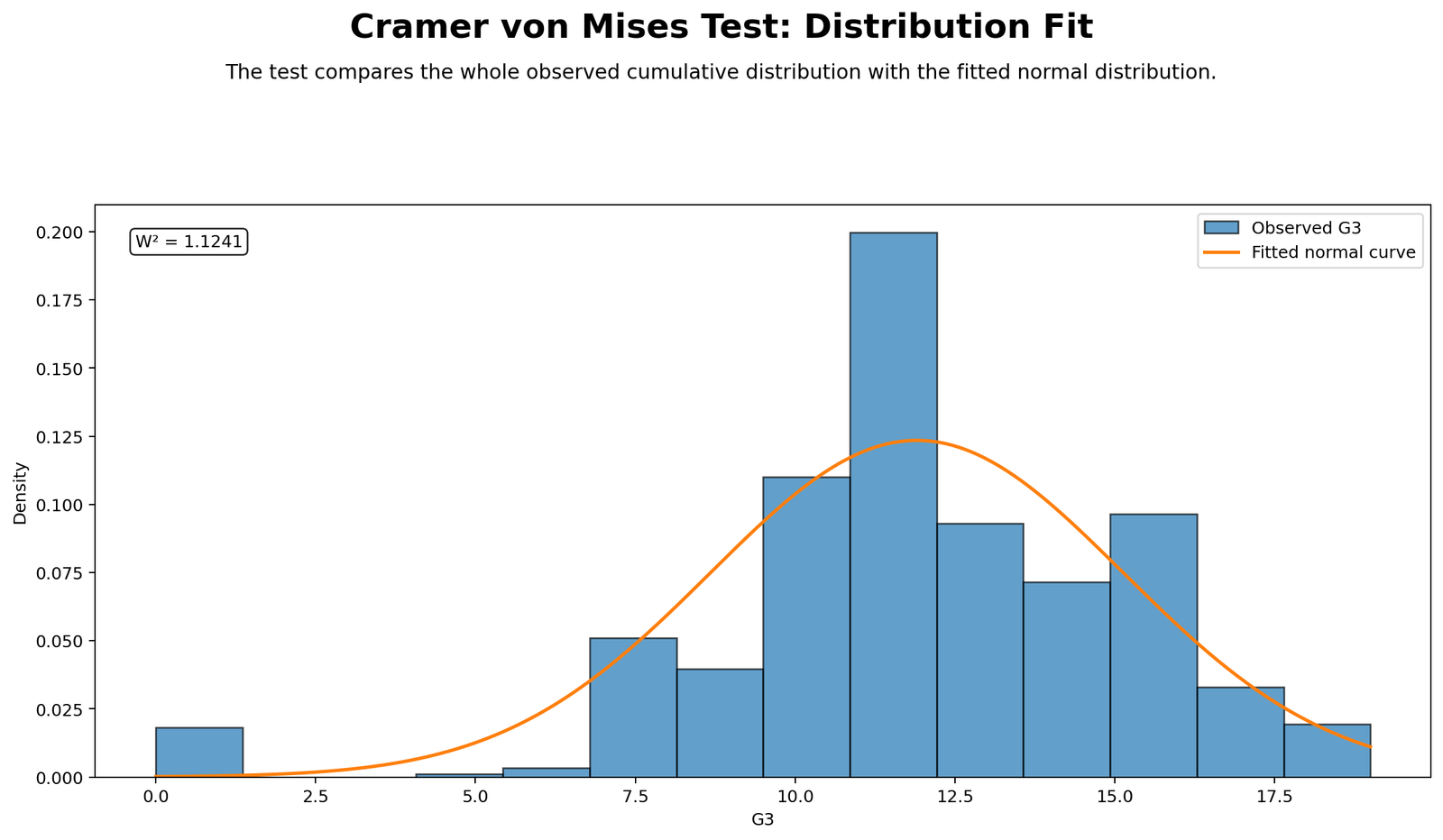
This chart shows the observed distribution of G3 final grades compared with a fitted normal distribution. The fitted normal curve is based on the sample mean and standard deviation. If the G3 data were normal, the histogram pattern would closely follow the fitted curve across the center and tails.
The Cramer von Mises result indicates that the visual fit is not close enough across the full distribution. Some grade values may cluster more heavily than the fitted normal curve expects, while other areas may show gaps or tail differences. These distribution-wide differences contribute to the significant W2 statistic.
Decision/reporting conclusion: Report that the distribution fit chart supports the formal test result. The observed G3 distribution does not align perfectly with the fitted normal curve, and the Cramer von Mises Test rejects normality.
Python Chart 2: Empirical CDF vs Fitted Normal CDF
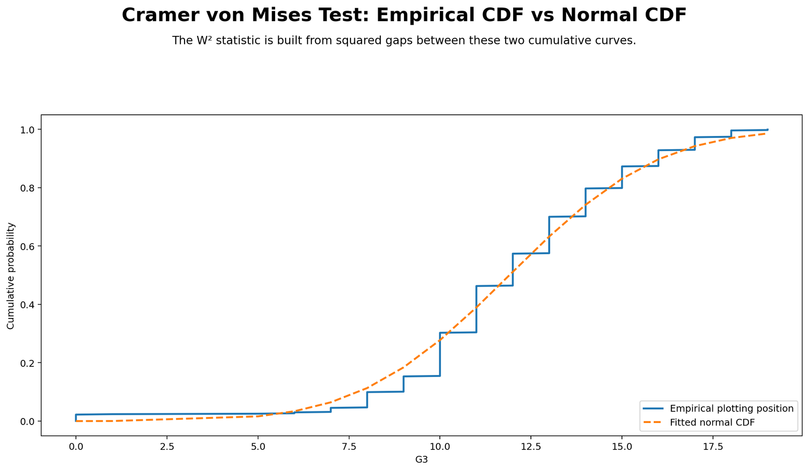
This empirical CDF chart is central to understanding the Cramer von Mises Test. The empirical CDF shows the cumulative proportion of observed G3 values, while the fitted normal CDF shows what those cumulative proportions would look like if the data followed the fitted normal distribution.
When the two CDF lines are close, the W2 statistic is small. When the empirical CDF repeatedly departs from the fitted normal CDF, the squared gap accumulates. The verified result W2 = 1.1241 indicates that the total squared gap is large enough to reject the normality null hypothesis.
Decision/reporting conclusion: Report that the empirical CDF differs meaningfully from the fitted normal CDF. This chart visually explains why the Cramer von Mises Test is significant.
Python Chart 3: Normal Q-Q Plot
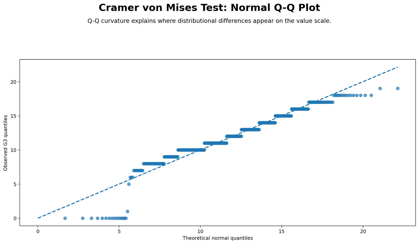
The normal Q-Q plot compares observed quantiles with expected normal quantiles. If the data are approximately normal, the points should fall close to the reference line. Systematic curvature, tail departures or grouped steps indicate departure from normality.
This Q-Q plot supports the Cramer von Mises result by showing where the G3 distribution deviates from normality. Because G3 is a grade variable, it may have discreteness, ceiling/floor behavior or clustered values. These features can create visible Q-Q departures and contribute to a significant goodness-of-fit test.
Decision/reporting conclusion: Report that the Q-Q plot provides visual confirmation of the formal Cramer von Mises decision. The distribution is not perfectly normal, especially where points depart from the reference line.
Python Chart 4: Squared CDF Gap Contributions
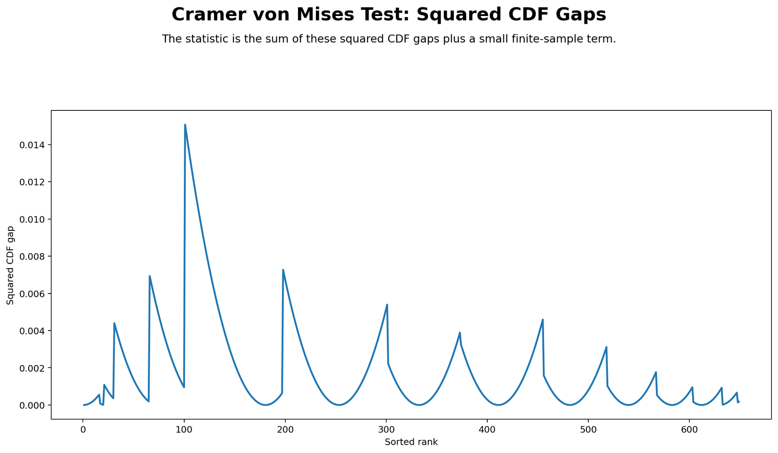
This chart explains the mechanics of the Cramer von Mises statistic. Each ordered observation contributes a squared gap between the fitted normal CDF and the empirical plotting position. Larger bars or higher contribution regions show where the empirical distribution differs most from the fitted normal distribution.
This plot is very useful for interpretation because it shows that W2 is not just an abstract number. It is built from many small squared differences across the distribution. If some sections of the distribution contribute much more than others, those sections explain the main source of non-normality.
Decision/reporting conclusion: Report that the squared CDF gap chart identifies where the fitted normal distribution fails most strongly. The accumulated gap produces W2 = 1.1241, supporting rejection of normality.
Python Chart 5: Monte Carlo Reference Distribution
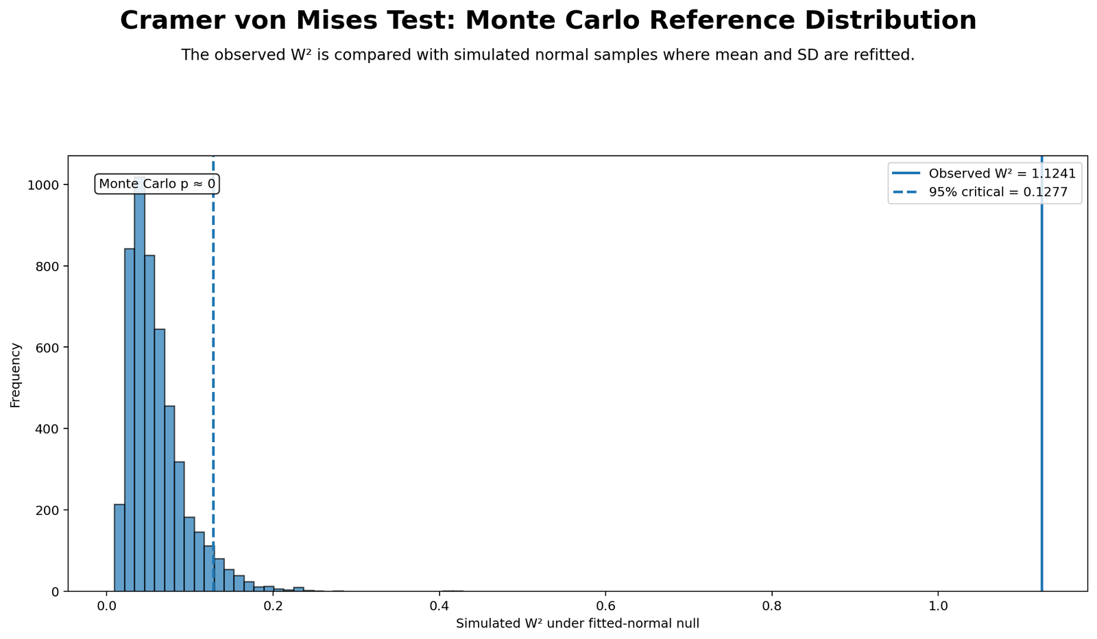
The Monte Carlo reference distribution chart compares the observed W2 statistic with the W2 values expected under normality. Simulated samples are generated from the fitted normal model, W2 is calculated for each simulated sample, and the observed statistic is placed against that reference distribution.
Because the observed result has Monte Carlo p ≈ 0.00002, the observed W2 is far into the extreme tail of the reference distribution. This means that a W2 value as large as the observed result would be very unlikely if the G3 data truly followed the fitted normal distribution.
Decision/reporting conclusion: Report that the Monte Carlo reference distribution strongly supports rejection of normality. The observed W2 is extreme relative to the simulated normal reference distribution.
Python Chart 6: W2 Across Variables
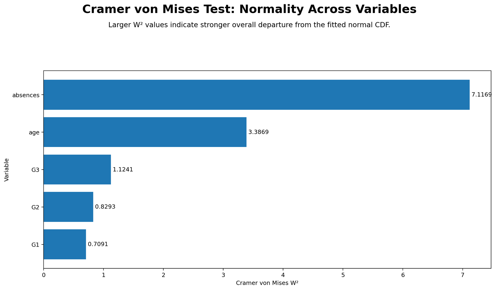
This chart compares W2 values across variables. It helps answer a broader diagnostic question: which variable is closest to normal, and which variable departs most strongly? A higher W2 indicates a larger distribution-wide gap from the fitted normal distribution.
For student performance data, grade variables and count variables may behave differently. A count variable such as absences may show strong right-skewness, while a grade variable may show clustering, ceiling/floor effects or discrete score patterns. This chart helps decide which variables need transformation, nonparametric alternatives or robust methods.
Decision/reporting conclusion: Report the relative W2 pattern across variables. Variables with higher W2 values show stronger normality departures and deserve closer visual and statistical review.
Python Chart 7: Group W2 Comparison
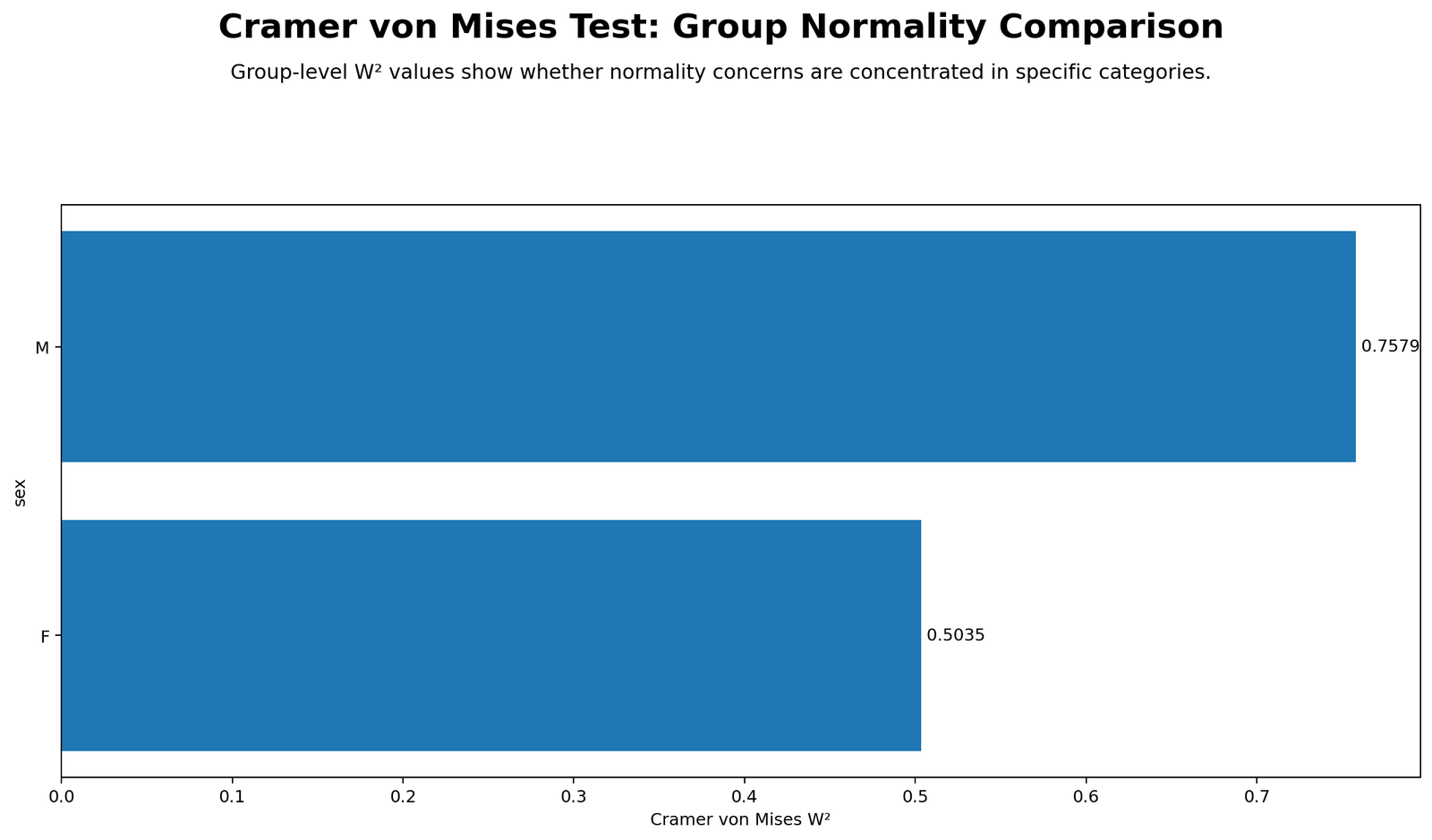
The group W2 comparison chart shows whether distributional fit differs across groups. For example, normality may be closer in one school, sex category or study-time group than another. This is useful because a full-sample normality test can hide subgroup differences.
If one group has a much higher W2 statistic, that group contributes more strongly to the overall normality departure. The analyst should inspect that group with histograms, Q-Q plots and descriptive statistics. Group-level distribution differences may also affect comparisons, confidence intervals and regression assumptions.
Decision/reporting conclusion: Report whether normality departure is similar across groups or concentrated in specific groups. If one group has a much larger W2, discuss that subgroup in the diagnostic interpretation.
R Chart-by-Chart Validation
The R charts validate the Python Cramer von Mises Test workflow using a separate statistical environment. This is useful for reproducibility because the same conclusion is supported by both Python and R outputs.
R Chart 1: Distribution Fit for Cramer von Mises Test
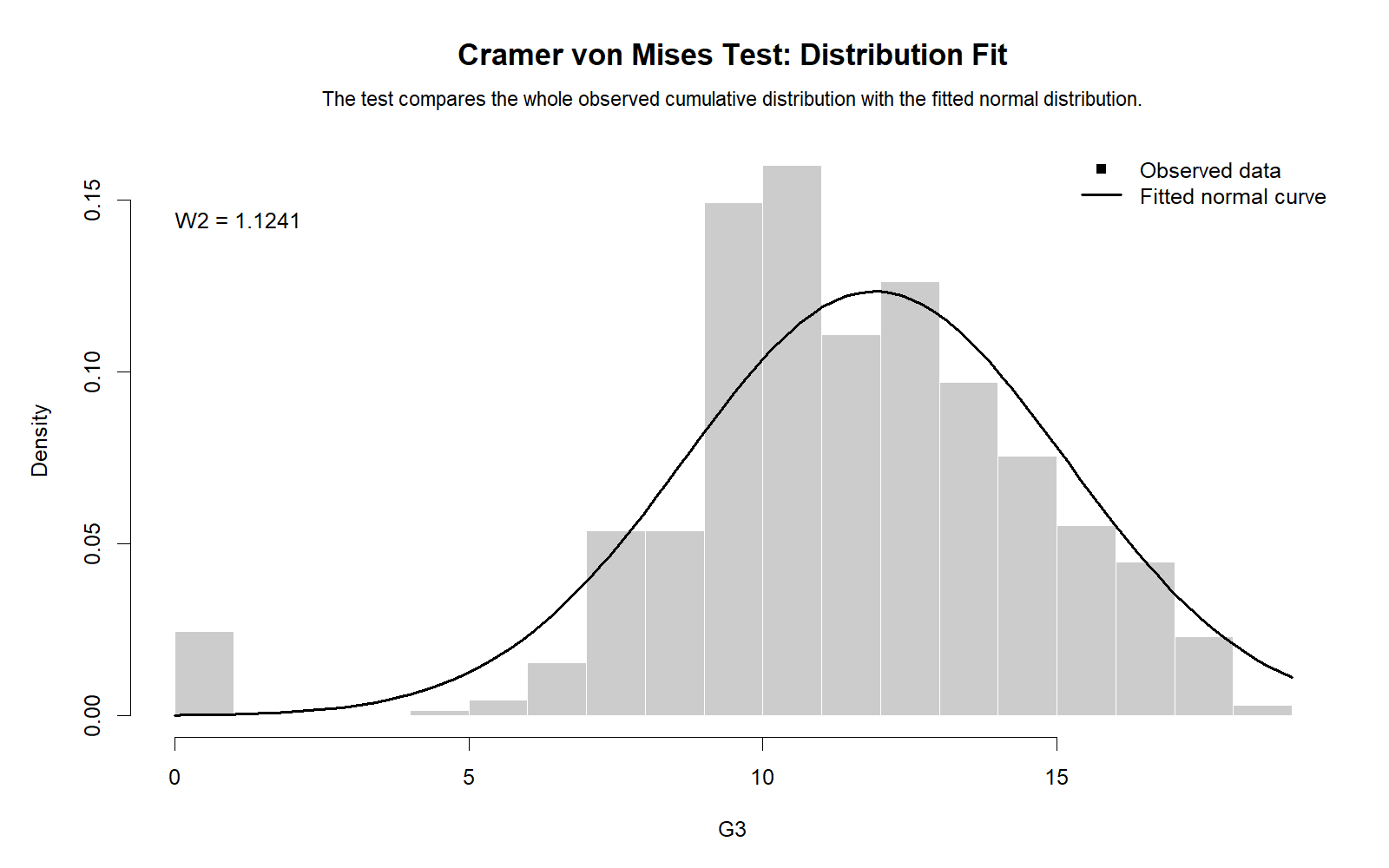
The R distribution fit chart validates the Python histogram and fitted normal curve. It shows whether the observed grade distribution visually follows the theoretical normal shape. The significant test result indicates that the visual departures are large enough to reject normality.
Decision/reporting conclusion: Report that the R distribution fit chart confirms the Python interpretation: the observed distribution does not match the fitted normal distribution closely enough.
R Chart 2: Empirical CDF vs Fitted Normal CDF
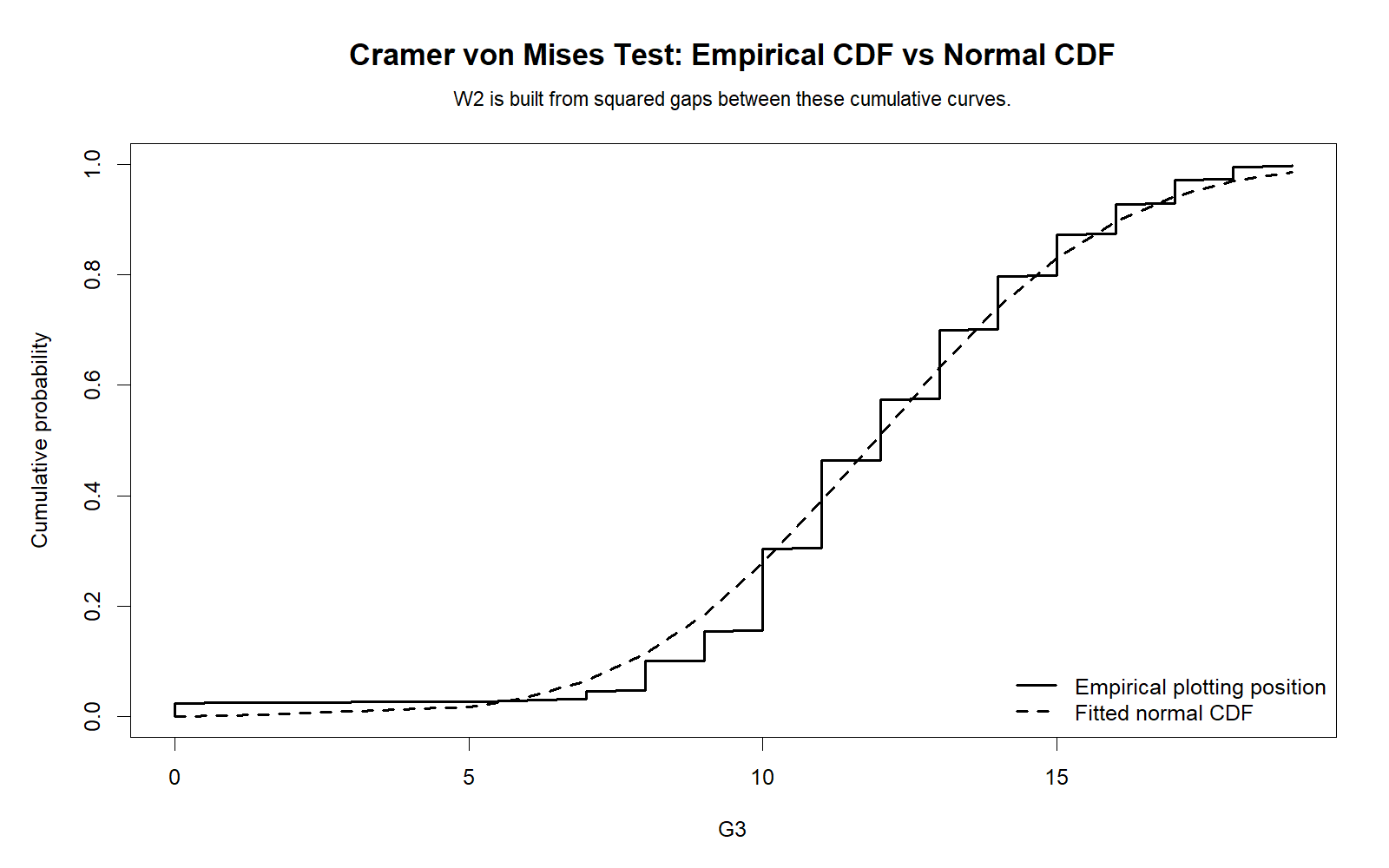
The R empirical CDF chart confirms the distribution-wide gap between the observed cumulative distribution and the fitted normal cumulative distribution. This chart directly supports the logic of the Cramer von Mises W2 statistic.
Decision/reporting conclusion: Report that the R empirical CDF plot validates the CDF-gap interpretation. The empirical distribution deviates enough from the fitted normal distribution to support rejecting H0.
R Chart 3: Normal Q-Q Plot
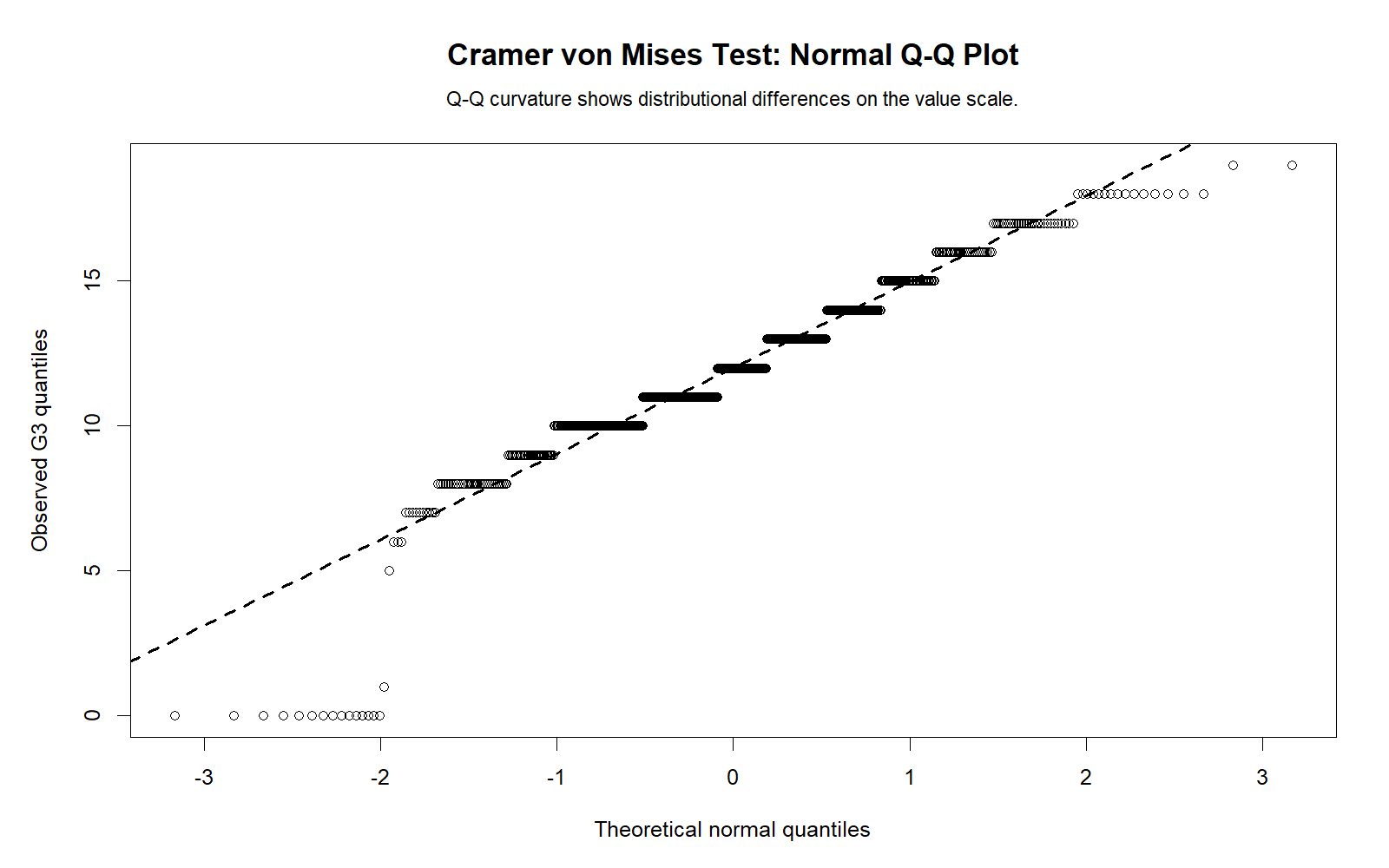
The R Q-Q plot confirms whether deviations from normality appear in the same way as the Python Q-Q plot. Points departing from the line indicate that the observed distribution does not follow the expected normal quantile pattern.
Decision/reporting conclusion: Report that the R Q-Q plot confirms the visual non-normality pattern. This supports the statistically significant Cramer von Mises decision.
R Chart 4: Squared CDF Gap Contributions
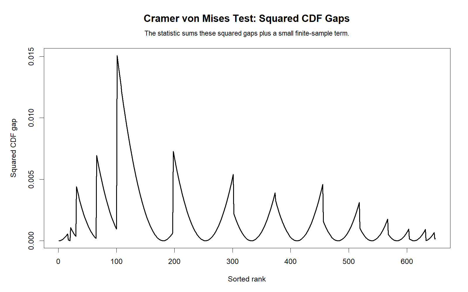
The R squared CDF gap chart validates the Python contribution plot. It shows where the empirical distribution and fitted normal distribution differ most. These squared differences are the building blocks of the W2 statistic.
Decision/reporting conclusion: Report that the R gap-contribution chart supports the same explanation of W2: the rejection of normality comes from accumulated distribution-wide CDF differences.
R Chart 5: Monte Carlo Reference Distribution
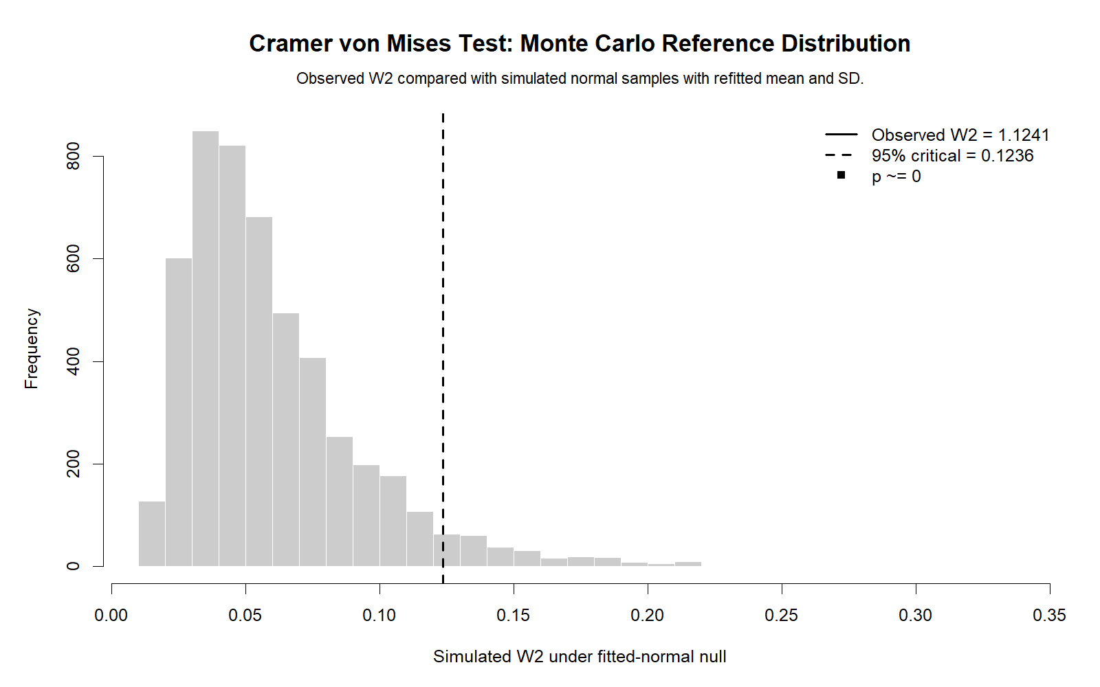
The R Monte Carlo reference distribution confirms the p-value logic. If the observed W2 falls far in the tail of simulated W2 values, the normality assumption is unlikely. This matches the verified Monte Carlo p-value of approximately 0.00002.
Decision/reporting conclusion: Report that R confirms the observed W2 is extreme under the simulated normal reference distribution. The normality null hypothesis should be rejected.
R Chart 6: W2 Across Variables
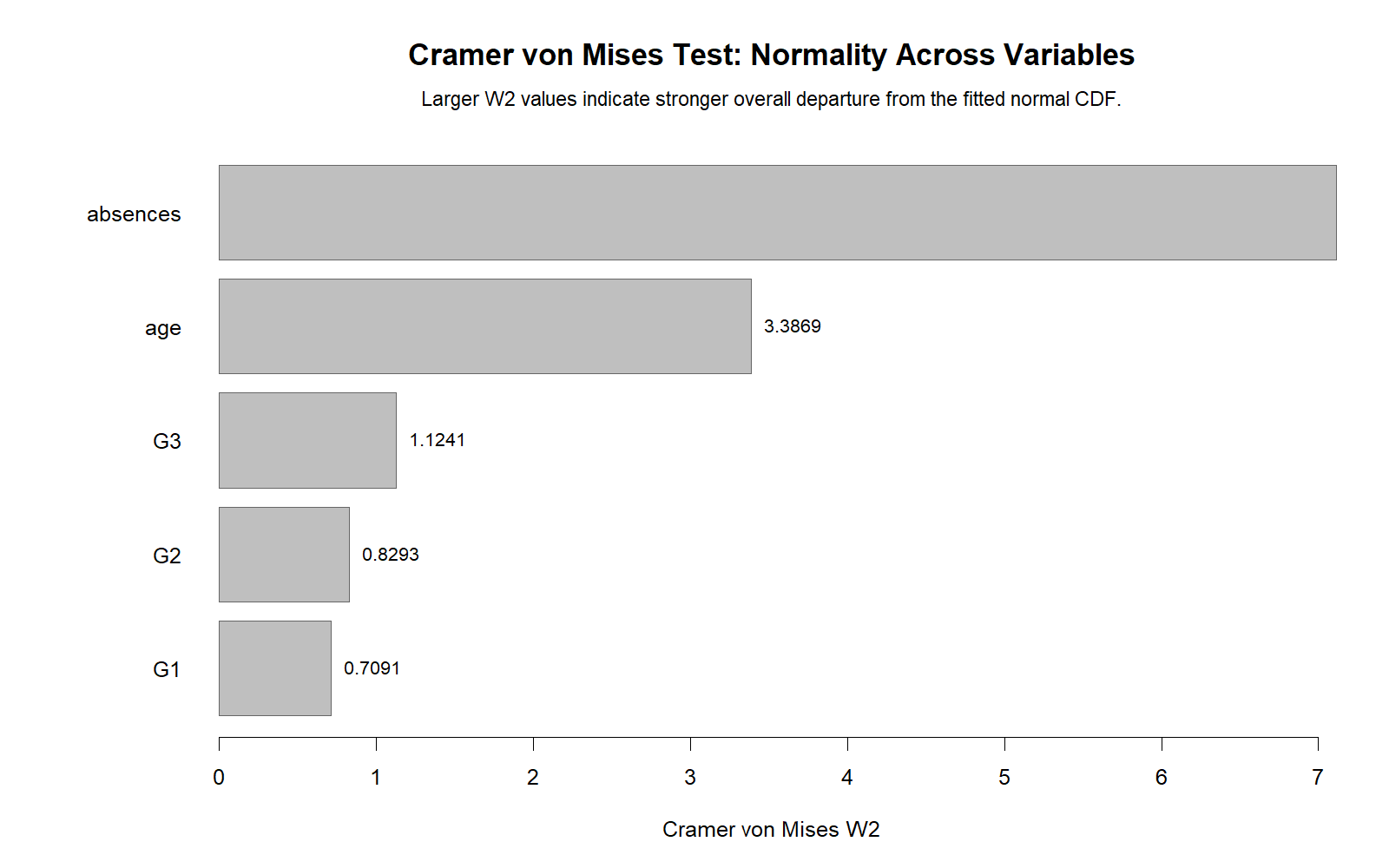
The R W2-across-variables chart validates the Python comparison of distributional fit across variables. This is helpful when the analyst needs to decide which variables require transformation, robust methods or nonparametric alternatives.
Decision/reporting conclusion: Report that the R variable comparison confirms which variables show the largest Cramer von Mises departures from fitted normality.
R Chart 7: Group W2 Comparison
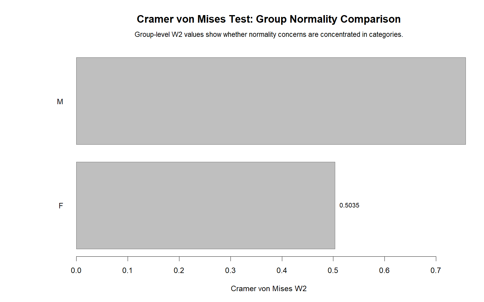
The R group W2 chart validates the subgroup diagnostic comparison. If one group shows a larger W2 value, the group may have stronger distributional departure from normality. This can affect group comparison methods, model assumptions and interpretation.
Decision/reporting conclusion: Report whether R confirms the same group-level pattern as Python. If some groups depart more strongly from normality, discuss those groups in the diagnostic conclusion.
SPSS, R, Python and Excel Workflows for the Cramer von Mises Test
The Cramer von Mises workflow is based on sorting the data, fitting the target distribution, calculating theoretical CDF values, comparing them with empirical plotting positions, and estimating the p-value. Python and R are the strongest tools for direct implementation, SPSS can support the workflow with computed variables and exported output, and Excel can be used for a transparent manual calculation.
SPSS Workflow
| Step | SPSS Menu or Syntax | Purpose |
|---|---|---|
| Open dataset | File > Open > Data | Load the SPSS-ready dataset. |
| Inspect descriptives | Analyze > Descriptive Statistics > Descriptives / Explore | Obtain N, mean, standard deviation, histogram and Q-Q plot. |
| Sort variable | Sort Cases | Order the data from smallest to largest. |
| Compute fitted normal CDF | Use CDF.NORMAL in Compute Variable | Calculate theoretical CDF values using sample mean and standard deviation. |
| Compute empirical plotting position | Use case rank and sample size | Create empirical CDF comparison values. |
| Compute squared gap | Compute squared difference | Calculate Cramer von Mises contribution terms. |
| Export output | OUTPUT EXPORT | Save SPSS output PDF for reporting. |
Python Workflow
| Step | Python Action | Purpose |
|---|---|---|
| Read data | pandas.read_csv() | Load the dataset into a DataFrame. |
| Select variable | df["G3"].dropna() | Prepare the tested variable. |
| Estimate parameters | mean() and std() | Fit the normal distribution using sample mean and SD. |
| Compute W2 | Manual formula or SciPy method | Calculate the Cramer von Mises statistic. |
| Run Monte Carlo | Simulate normal samples | Estimate p-value when parameters are estimated from data. |
| Create charts | matplotlib | Generate distribution, CDF, Q-Q, squared gap and Monte Carlo plots. |
R Workflow
| Step | R Action | Purpose |
|---|---|---|
| Read data | read.csv() | Load the dataset. |
| Select variable | x <- df$G3 | Prepare the tested variable. |
| Estimate normal parameters | mean(x), sd(x) | Fit the normal CDF. |
| Compute W2 | Manual formula or package function | Calculate the Cramer von Mises statistic. |
| Simulate reference distribution | replicate() | Estimate Monte Carlo p-value. |
| Build charts | ggplot2 | Create validation charts. |
Excel Workflow
| Excel Task | Formula or Tool | Purpose |
|---|---|---|
| Sort the variable | Data > Sort Smallest to Largest | Prepare ordered observations. |
| Calculate mean | =AVERAGE(A2:A650) | Fit normal location parameter. |
| Calculate standard deviation | =STDEV.S(A2:A650) | Fit normal scale parameter. |
| Fitted normal CDF | =NORM.DIST(A2,$H$1,$H$2,TRUE) | Compute theoretical CDF value. |
| Empirical plotting position | =(2*ROW(A1)-1)/(2*$H$3) | Compute empirical CDF comparison value. |
| Squared gap | =(B2-C2)^2 | Compute W2 contribution. |
| W2 statistic | =1/(12*n)+SUM(squared gaps) | Calculate Cramer von Mises statistic. |
Code Blocks for Cramer von Mises Test
SPSS Syntax for Cramer von Mises Test Support
* Cramer von Mises Test support in SPSS.
* Main variable: G3 final grade.

TITLE "Cramer von Mises Test: Normality and empirical CDF comparison".

DATASET ACTIVATE DataSet1.

* Inspect descriptive statistics and normality plots.
EXAMINE VARIABLES=G3
  /PLOT BOXPLOT HISTOGRAM NPPLOT
  /COMPARE GROUPS
  /STATISTICS DESCRIPTIVES
  /CINTERVAL 95
  /MISSING LISTWISE
  /NOTOTAL.

* Sort cases by G3 for empirical CDF workflow.
SORT CASES BY G3 (A).

* Create case index after sorting.
COMPUTE cvm_i = $CASENUM.
EXECUTE.

* Replace 649 with the valid sample size if your dataset changes.
COMPUTE cvm_n = 649.

* Use verified sample mean and standard deviation for fitted normal CDF.
COMPUTE cvm_mean = 11.9060.
COMPUTE cvm_sd = 3.2307.

* Empirical plotting position: (2i - 1)/(2n).
COMPUTE empirical_pos = ((2*cvm_i)-1)/(2*cvm_n).

* Fitted normal CDF.
COMPUTE fitted_norm_cdf = CDF.NORMAL(G3,cvm_mean,cvm_sd).

* Squared gap contribution.
COMPUTE squared_cdf_gap = (fitted_norm_cdf - empirical_pos)**2.
EXECUTE.

DESCRIPTIVES VARIABLES=G3 fitted_norm_cdf empirical_pos squared_cdf_gap
  /STATISTICS=MEAN STDDEV MIN MAX SUM.

* The W2 statistic is:
* W2 = 1/(12*n) + SUM(squared_cdf_gap).
* Verified result for this guide: W2 = 1.1241, Monte Carlo p approximately .00002.

OUTPUT EXPORT
  /CONTENTS EXPORT=VISIBLE
  /PDF DOCUMENTFILE="Cramer-von-Mises-Test-SPSS-Output.pdf".
Python Code for Cramer von Mises Test
import numpy as np
import pandas as pd
import matplotlib.pyplot as plt
from scipy import stats

# Load dataset
df = pd.read_csv("dataset.csv")

# Main variable
x = pd.to_numeric(df["G3"], errors="coerce").dropna().to_numpy()
x = np.sort(x)

n = len(x)
mu = np.mean(x)
sd = np.std(x, ddof=1)

# Fitted normal CDF values
fitted_cdf = stats.norm.cdf(x, loc=mu, scale=sd)

# Empirical plotting positions
i = np.arange(1, n + 1)
empirical_pos = (2 * i - 1) / (2 * n)

# Cramer von Mises W2 statistic
squared_gaps = (fitted_cdf - empirical_pos) ** 2
w2 = (1 / (12 * n)) + np.sum(squared_gaps)

print("N:", n)
print("Mean:", mu)
print("SD:", sd)
print("Cramer von Mises W2:", w2)

# Monte Carlo p-value with parameter re-estimation
rng = np.random.default_rng(12345)
B = 50000
sim_w2 = np.empty(B)

for b in range(B):
    sim = rng.normal(mu, sd, n)
    sim = np.sort(sim)
    sim_mu = np.mean(sim)
    sim_sd = np.std(sim, ddof=1)
    sim_cdf = stats.norm.cdf(sim, loc=sim_mu, scale=sim_sd)
    sim_gaps = (sim_cdf - empirical_pos) ** 2
    sim_w2[b] = (1 / (12 * n)) + np.sum(sim_gaps)

p_value = np.mean(sim_w2 >= w2)
print("Monte Carlo p-value:", p_value)

# Chart 1: Distribution fit
plt.figure(figsize=(8, 6))
plt.hist(x, bins=20, density=True, alpha=0.7)
grid = np.linspace(min(x), max(x), 300)
plt.plot(grid, stats.norm.pdf(grid, mu, sd), linewidth=2)
plt.xlabel("G3 final grade")
plt.ylabel("Density")
plt.title("Distribution Fit: Cramer von Mises Test")
plt.tight_layout()
plt.savefig("cramer-von-mises-test-python-01-chart_01_distribution_fit_cramer_von_mises.png", dpi=300)
plt.close()

# Chart 2: Empirical CDF vs fitted normal CDF
ecdf = np.arange(1, n + 1) / n
plt.figure(figsize=(8, 6))
plt.step(x, ecdf, where="post", label="Empirical CDF")
plt.plot(x, fitted_cdf, label="Fitted normal CDF")
plt.xlabel("G3 final grade")
plt.ylabel("Cumulative probability")
plt.title("Empirical CDF vs Fitted Normal CDF")
plt.legend()
plt.tight_layout()
plt.savefig("cramer-von-mises-test-python-02-chart_02_empirical_cdf_vs_fitted_normal_cdf.png", dpi=300)
plt.close()

# Chart 3: Normal Q-Q plot
plt.figure(figsize=(8, 6))
stats.probplot(x, dist="norm", plot=plt)
plt.title("Normal Q-Q Plot")
plt.tight_layout()
plt.savefig("cramer-von-mises-test-python-03-chart_03_normal_qq_plot.png", dpi=300)
plt.close()

# Chart 4: Squared CDF gap contributions
plt.figure(figsize=(9, 5))
plt.plot(i, squared_gaps)
plt.xlabel("Ordered case")
plt.ylabel("Squared CDF gap")
plt.title("Squared CDF Gap Contributions")
plt.tight_layout()
plt.savefig("cramer-von-mises-test-python-04-chart_04_squared_cdf_gap_contributions.png", dpi=300)
plt.close()

# Chart 5: Monte Carlo reference distribution
plt.figure(figsize=(8, 6))
plt.hist(sim_w2, bins=40, alpha=0.7)
plt.axvline(w2, linewidth=2)
plt.xlabel("Simulated W2")
plt.ylabel("Frequency")
plt.title("Monte Carlo Reference Distribution")
plt.tight_layout()
plt.savefig("cramer-von-mises-test-python-05-chart_05_monte_carlo_reference_distribution.png", dpi=300)
plt.close()
R Code for Cramer von Mises Test
# Cramer von Mises Test in R

library(ggplot2)

df <- read.csv("dataset.csv")

x <- as.numeric(df$G3)
x <- sort(x[!is.na(x)])

n <- length(x)
mu <- mean(x)
sd_x <- sd(x)

i <- 1:n
empirical_pos <- (2*i - 1)/(2*n)
fitted_cdf <- pnorm(x, mean = mu, sd = sd_x)
squared_gaps <- (fitted_cdf - empirical_pos)^2

w2 <- (1/(12*n)) + sum(squared_gaps)

cat("N:", n, "\n")
cat("Mean:", mu, "\n")
cat("SD:", sd_x, "\n")
cat("Cramer von Mises W2:", w2, "\n")

# Monte Carlo p-value with parameter re-estimation
set.seed(12345)
B <- 50000
sim_w2 <- numeric(B)

for (b in 1:B) {
  sim <- sort(rnorm(n, mean = mu, sd = sd_x))
  sim_mu <- mean(sim)
  sim_sd <- sd(sim)
  sim_cdf <- pnorm(sim, mean = sim_mu, sd = sim_sd)
  sim_gaps <- (sim_cdf - empirical_pos)^2
  sim_w2[b] <- (1/(12*n)) + sum(sim_gaps)
}

p_value <- mean(sim_w2 >= w2)
cat("Monte Carlo p-value:", p_value, "\n")

plot_df <- data.frame(
  x = x,
  ecdf = (1:n)/n,
  fitted_cdf = fitted_cdf,
  case = i,
  squared_gap = squared_gaps
)

# Chart 1: Distribution fit
ggplot(data.frame(x=x), aes(x=x)) +
  geom_histogram(aes(y=after_stat(density)), bins=20, alpha=.7) +
  stat_function(fun=dnorm, args=list(mean=mu, sd=sd_x), linewidth=1) +
  labs(title="Distribution Fit: Cramer von Mises Test",
       x="G3 final grade", y="Density")

# Chart 2: Empirical CDF vs fitted normal CDF
ggplot(plot_df, aes(x=x)) +
  geom_step(aes(y=ecdf), linewidth=1) +
  geom_line(aes(y=fitted_cdf), linewidth=1) +
  labs(title="Empirical CDF vs Fitted Normal CDF",
       x="G3 final grade", y="Cumulative probability")

# Chart 3: Normal Q-Q plot
qqnorm(x)
qqline(x)

# Chart 4: Squared CDF gap contributions
ggplot(plot_df, aes(x=case, y=squared_gap)) +
  geom_line() +
  labs(title="Squared CDF Gap Contributions",
       x="Ordered case", y="Squared CDF gap")

# Chart 5: Monte Carlo reference distribution
ggplot(data.frame(sim_w2=sim_w2), aes(x=sim_w2)) +
  geom_histogram(bins=40, alpha=.7) +
  geom_vline(xintercept=w2, linewidth=1) +
  labs(title="Monte Carlo Reference Distribution",
       x="Simulated W2", y="Frequency")
Excel Formulas for Cramer von Mises Test
Assume sorted G3 values are in A2:A650.

Mean in H1:
=AVERAGE(A2:A650)

Standard deviation in H2:
=STDEV.S(A2:A650)

Sample size in H3:
=COUNT(A2:A650)

Case index in B2:
=ROW(A1)

Empirical plotting position in C2:
=(2*B2-1)/(2*$H$3)

Fitted normal CDF in D2:
=NORM.DIST(A2,$H$1,$H$2,TRUE)

Squared CDF gap in E2:
=(D2-C2)^2

Copy B2:E2 down to the last observation.

Cramer von Mises W2 statistic:
=1/(12*$H$3)+SUM(E2:E650)

Decision:
If the Monte Carlo or reference p-value is below .05, reject normality.
If the p-value is .05 or above, do not reject normality.
APA Reporting Wording for the Cramer von Mises Test
When reporting the Cramer von Mises Test, include the tested variable, sample size, fitted distribution, W2 statistic, p-value and decision. Also include a visual interpretation based on the distribution fit chart, empirical CDF chart and Q-Q plot.
APA-Style Report
A Cramer von Mises goodness-of-fit test was conducted to evaluate whether the G3 final grade variable followed a fitted normal distribution. The sample included 649 valid observations, with mean = 11.9060 and standard deviation = 3.2307. The test indicated a statistically significant departure from normality, W2 = 1.1241, Monte Carlo p ≈ 0.00002. Therefore, the null hypothesis of normality was rejected. Visual inspection of the empirical CDF plot and normal Q-Q plot also supported the conclusion that G3 did not closely follow the fitted normal distribution.
Short Report Sentence
The Cramer von Mises Test showed that G3 final grades significantly departed from the fitted normal distribution, W2 = 1.1241, Monte Carlo p ≈ 0.00002. Therefore, the normality assumption was rejected for G3.
Student-Friendly Report Example
The Cramer von Mises Test compares the observed cumulative distribution with the expected normal cumulative distribution. In this example, the p-value was much smaller than .05, so the G3 scores were not normally distributed. The charts show that the empirical CDF and fitted normal CDF do not match closely enough.
Common Mistakes in Cramer von Mises Test Interpretation
| Mistake | Why It Is a Problem | Correct Practice |
|---|---|---|
| Thinking the test only checks the tails | The Cramer von Mises Test accumulates squared CDF gaps across the full distribution. | Interpret the whole empirical CDF versus fitted CDF pattern. |
| Using only the p-value | A significant p-value does not explain where the distribution differs. | Use histograms, CDF plots, Q-Q plots and squared gap charts. |
| Ignoring sample size | Large samples can detect small deviations from normality. | Interpret p-values with visual diagnostics and practical importance. |
| Confusing Cramer von Mises with Kolmogorov-Smirnov | The Kolmogorov-Smirnov test focuses on the maximum CDF distance, while Cramer von Mises accumulates squared distances. | Choose the test based on the type of goodness-of-fit evidence needed. |
| Forgetting parameter estimation | If mean and standard deviation are estimated from the sample, reference p-values may need adjustment. | Use simulation or an appropriate implementation for estimated parameters. |
| Calling non-normality a failure of the whole study | Many methods are robust, especially with large samples. | Consider transformation, robust methods, nonparametric methods or model-based alternatives where needed. |
Key reminder: The Cramer von Mises Test is a diagnostic tool. It helps you understand distribution fit, but final analysis decisions should also consider research design, sample size, visual plots, assumptions and the planned statistical method.
When to Use the Cramer von Mises Test
Use the Cramer von Mises Test when you want to compare a sample distribution with a theoretical distribution across the whole cumulative distribution. It is commonly used for normality testing, but it can also be used as a broader goodness-of-fit tool.
| Use Case | Why Cramer von Mises Helps | Example from This Guide |
|---|---|---|
| Normality testing | Compares empirical CDF with fitted normal CDF. | G3 normality was rejected with W2 = 1.1241. |
| Goodness-of-fit checking | Evaluates distribution-wide fit. | Observed G3 distribution differed from fitted normal distribution. |
| Visual diagnostic support | Works well with CDF plots, Q-Q plots and histograms. | Python and R charts show why p was significant. |
| Comparing variables | W2 can be compared across variables for diagnostic screening. | W2 across variables chart identifies stronger departures. |
| Comparing groups | Group W2 values show whether distribution fit differs by subgroup. | Group W2 comparison chart supports subgroup interpretation. |
If the Cramer von Mises Test rejects normality and the planned method requires stronger normality support, consider transformation, robust methods or nonparametric alternatives. For transformation context, see reciprocal transformation. For comparison with hypothesis testing and reporting, see one-tailed t-test, one-sample z-test, one-proportion z-test, confidence interval, and effect size.
Downloads and Resources for Cramer von Mises Test
The resources below include the verified SPSS output PDF, Python charts and R validation charts used in this guide. These files support direct reporting, teaching, WordPress publishing and normality diagnostics practice.
Download SPSS Output PDF
Verified SPSS output for Cramer von Mises Test and normality interpretation.
Copy Cramer von Mises Code
Use SPSS, Python, R and Excel code blocks to reproduce the workflow.
Python Empirical CDF Chart
Empirical CDF versus fitted normal CDF for the Cramer von Mises Test.
R Monte Carlo Reference Chart
R validation chart showing the observed W2 against simulated W2 values.
FAQs About the Cramer von Mises Test
What is the Cramer von Mises Test?
The Cramer von Mises Test is a goodness-of-fit test that compares the empirical cumulative distribution function of a sample with a theoretical cumulative distribution function, such as the normal distribution.
What does the Cramer von Mises W2 statistic mean?
The W2 statistic measures the accumulated squared difference between the empirical CDF and the fitted theoretical CDF. Larger W2 values indicate stronger departure from the fitted distribution.
What was the result in this Cramer von Mises Test example?
The verified result for G3 final grade was N = 649, mean = 11.9060, standard deviation = 3.2307, W2 = 1.1241, and Monte Carlo p ≈ 0.00002. The normality null hypothesis was rejected.
How is the Cramer von Mises Test different from the Kolmogorov-Smirnov test?
The Kolmogorov-Smirnov test focuses on the maximum distance between the empirical and theoretical CDFs, while the Cramer von Mises Test accumulates squared differences across the whole distribution.
Does a significant Cramer von Mises Test mean my analysis is invalid?
No. A significant result means the tested distribution differs from the fitted distribution. You should consider sample size, plots, robustness, transformations, nonparametric methods or whether the planned statistical method can tolerate non-normality.
Can SPSS run the Cramer von Mises Test?
SPSS can support the workflow by calculating descriptives, fitted CDF values, empirical positions and squared CDF gaps. Python and R are usually more direct for the full statistic and Monte Carlo p-value.
Why use a Monte Carlo p-value for the Cramer von Mises Test?
A Monte Carlo p-value is useful when parameters such as the mean and standard deviation are estimated from the sample. Simulation creates a reference distribution that matches the practical testing setup.
Should I use charts with the Cramer von Mises Test?
Yes. Use distribution fit charts, empirical CDF plots, Q-Q plots, squared CDF gap charts and Monte Carlo reference plots. These visuals explain why the test is significant or not significant.
Can the Cramer von Mises Test be used across groups?
Yes. You can calculate W2 separately for groups and compare which group departs more strongly from the fitted distribution. Group W2 charts help explain subgroup differences in distribution fit.
What should I report in APA style?
Report the tested variable, sample size, fitted distribution, W2 statistic, p-value and decision. Also mention whether visual plots supported the test result.

