
Spearman Brown Formula: 7 Essential Steps, Worked Example and Interpretation
The Spearman Brown formula, also called the Spearman-Brown prophecy formula, predicts how reliability is expected to change when a test, scale, rating protocol or repeated-measure design is lengthened or shortened with comparable measurement units. This complete guide explains the assumptions, direct and rearranged equations, split-half correction, a 649-pair worked example, target-reliability planning, interpretation, and reconciled Python, R, SPSS and Excel results.
649 paired scores
Observed r = 0.864982
Double-length prediction = 0.927603
Python + R + SPSS + Excel
The Spearman Brown formula predicts reliability of 0.927603 after doubling the test length.
In the worked example, the observed Pearson relationship between G1 and G2 is r = 0.8649816303 across 649 complete pairs. Setting the length multiplier to k = 2 gives ρnew = 2(0.8649816303) / [1 + (2 − 1)(0.8649816303)] = 0.9276033782. Reversing the Spearman Brown formula shows that a multiplier of 1.4048452414 is required to reach a target reliability of 0.90, provided the added material behaves like the original material.
What does the Spearman Brown formula measure?
A reliability prediction for a declared proportional change in comparable measurement length.
The Spearman Brown formula answers a planning question: if a measure becomes longer or shorter while its new material remains comparable with the original material, what reliability should be expected? Reliability generally improves when more parallel information is combined because random errors can partially average out. Reliability generally declines when information is removed because each observed score depends on fewer indicators. The relationship is nonlinear, so doubling a test does not double its reliability and a coefficient cannot exceed 1 merely because the length multiplier is large.
Prediction form
The prediction form starts with the reliability of a current score and a proposed length multiplier. A multiplier of 2 means twice as much comparable material; 1.5 means 50% more; 0.5 means half as much. The output is a predicted reliability coefficient for the revised test. This is the use most readers have in mind when they search for a Spearman Brown formula calculator, a Spearman Brown prophecy formula example, or instructions on how to calculate the Spearman Brown formula.
The formula is useful because it converts an abstract design choice into an interpretable reliability expectation before an expensive revised form is assembled. It can show, for example, that moving from .86 to .90 requires far less additional material than moving from .90 to .98.
Required-length form
The rearranged Spearman Brown formula begins with current reliability and a desired target. Its output is the factor by which test length would need to change under the parallel-material model. Multiplying that factor by the current number of items gives a planning estimate for the future number of items. When the result is not an integer, practical planning rounds upward because a partial item cannot normally be administered.
The required-length calculation should be followed by content review, item development, pilot testing and a new empirical reliability analysis. The formula does not know whether the proposed additions are well written, appropriately difficult or aligned with the construct.
The name is sometimes confused with Spearman rank correlation. The two procedures are not the same. Spearman rank correlation evaluates monotonic association between two variables, whereas the Spearman Brown formula predicts reliability after changing length or steps up the correlation between parallel halves to the estimated reliability of the whole test.
Search-intent clarification
Queries such as formula Spearman Brown, Spearman Brown correction formula, Spearman Brown reliability formula, Spearman-Brown formula for split-half method and Spearman Brown prophecy formula for split half reliability all point to the same mathematical family. “Prediction,” “prophecy” and “correction” emphasize different applications, but the core expression remains kρ/[1 + (k − 1)ρ].
When should you use the Spearman Brown formula?
Use it for test-length planning or split-half correction only when the starting coefficient and measurement units support the prediction.
Define the score
Identify the current test, composite or measurement protocol whose reliability is being used.
Specify the change
State whether the measure will be shortened, lengthened or reconstructed from two halves.
Defend comparability
Explain why added or retained material is expected to have similar quality and construct coverage.
Calculate the prediction
Apply the Spearman Brown formula with a clearly defined reliability and multiplier.
Verify empirically
Pilot the revised form and calculate reliability from the actual revised scores.
Test-length planning
Use the Spearman Brown prophecy formula when a current reliability estimate is available and a team is deciding whether to add or remove comparable items, trials, observations, occasions or ratings. Examples include expanding an educational test, reducing a survey burden, increasing repeated trials in a laboratory measure, or estimating how many equivalent indicators are needed for a target reliability.
The multiplier must describe the same unit of information used by the starting coefficient. If a 40-item test becomes 60 items, k = 60/40 = 1.5. If a protocol grows from three comparable ratings to five, k = 5/3.
Split-half correction
When a full test is split into two comparable halves, the correlation between the half scores describes agreement between half-length forms. For equal halves, setting k = 2 steps that half-test correlation up to an estimate for the whole test. This common application is why many courses call the method the Spearman Brown split half formula.
A single arbitrary split can be unstable. Different odd-even, first-second or random splits can produce different correlations. Strong analysis therefore considers the split design and may examine multiple splits rather than treating one convenient split as definitive.
Two-item or two-component scores
For a two-item standardized score, the Spearman-Brown coefficient based on the item correlation equals standardized coefficient alpha. It is often more informative to report the inter-item correlation and Spearman-Brown result than to discuss two-item alpha as though it represented a long scale. Raw alpha can differ slightly when the two components have unequal variances, as occurs in the worked example.
Do not automatically use this equivalence when components differ in scoring, scale, variance or substantive role.
Spearman Brown formula assumptions: conditions to check
The arithmetic is exact, but the reliability prediction depends on strong measurement-design assumptions.
Parallel or sufficiently comparable additions
The classical interpretation assumes that the added material behaves like a parallel replication of the current material: it targets the same construct, has comparable true-score properties and introduces a similar amount and type of error. Exact parallelism is demanding. In applied planning, the formula is commonly treated as an approximation, but the analyst should still explain why the new items or observations are expected to resemble those already used.
Adding easy, repetitive or poorly discriminating items may produce much less reliability improvement than predicted. Adding a different content domain may change what the total score means. Removing the most informative items may reduce reliability more than a simple proportional shortening predicts.
A defensible starting reliability
The input should be a reliability coefficient that matches the score and intended use. A test-retest coefficient, internal consistency estimate, parallel-forms coefficient or inter-rater coefficient describes a different error design. The same length multiplier can yield a numerical answer for any value between 0 and 1, but that answer is meaningful only when additional measurement would reduce the error represented by the starting coefficient.
The observed G1-G2 relationship in this worked example is used as a parallel-score demonstration. Because G1 and G2 are sequential educational grades rather than literal randomly split test halves, the result illustrates the computation and its conditions; it should not be generalized as the reliability of every grade measure.
Stable construct and administration
Length planning assumes the construct, population, administration conditions and scoring rules remain sufficiently stable. If a longer test creates fatigue, time pressure or disengagement, its error structure may differ. If a shorter form changes content balance, the revised score may no longer represent the same construct. Reliability is therefore a property of scores under defined conditions, not an immutable property of an item list.
Appropriate correlation model
The equal-half correction commonly uses Pearson correlation between continuous half scores. Severe range restriction, nonlinear relationships, influential outliers or mixed scoring scales can distort that correlation. Review the raw score relationship with tools such as scatterplots and correlation, outlier detection and the site’s correlation assumptions guide.
Consistent missing-data handling
The worked example uses all 649 complete G1-G2 pairs. If some respondents have one component but not the other, state whether pairwise deletion, listwise deletion, imputation or a model-based method was used. A reliability prediction from one subset should not be compared casually with a revised-test reliability from a different population.
No standalone null hypothesis
The Spearman Brown formula itself is an algebraic transformation, not a significance test. It does not test a null hypothesis that length has no effect, and it does not generate a p-value or confidence interval by itself. The SPSS output reports a significance test for the Pearson correlation and a paired-mean test, but those inferential results answer separate questions. A bootstrap or analytic uncertainty method must be specified if an interval for the predicted reliability is required.
Spearman Brown formula statistical meaning: prediction, not a p-value
State the design proposition correctly and separate reliability planning from significance testing.
The Spearman Brown formula is a deterministic reliability-planning equation rather than a null-hypothesis significance test. It does not produce a test statistic or p-value by itself. Its input is an observed or assumed reliability coefficient, and its output is a conditional prediction based on a declared length multiplier.
Prediction statement
Let ρold denote the reliability of the current score and let k denote the ratio of new measurement length to old measurement length. The equation predicts ρnew under the proposition that the added or retained units are sufficiently parallel to the current units.
This is a design prediction. It is not evidence that the revised score has already achieved the predicted coefficient.
Applied statements for this analysis
The appropriate language is therefore “predicted reliability,” “required length multiplier” and “conditional on comparable added material.” Avoid stating that the formula proves reliability improvement.
What can be evaluated statistically?
The starting coefficient can have a confidence interval, and competing reliability estimates can sometimes be compared with resampling or model-based methods. Those analyses concern uncertainty in the estimated input or observed reliability—not a p-value generated by the Spearman-Brown equation itself.
What must be evaluated substantively?
Construct coverage, item difficulty, discrimination, scoring consistency, fatigue, administration time and population fit determine whether the proportional-length assumption is credible. These design conditions are more important than treating the equation as a mechanical calculator.
Spearman Brown formula, symbols and rearranged equation
One equation predicts reliability after a length change; the rearranged equation estimates the required multiplier.
ρold is the current reliability or the correlation being stepped up, k is new length divided by old length, and ρnew is predicted reliability after the change. When two equal halves are combined, k = 2.
This rearranged Spearman Brown formula gives the factor by which length must change to reach a declared target under the same comparability assumptions.
Shortening
For k = 0.5, the worked coefficient declines from 0.864982 to 0.762086. Reliability does not fall by exactly half because the formula transforms the ratio of true-score and error components rather than applying a simple percentage reduction to the coefficient.
Lengthening
For k = 1.5, predicted reliability is 0.905746; for k = 2, it is 0.927603; and for k = 3, it is 0.950542. Each additional unit of proportional length produces a smaller marginal gain as reliability approaches 1.
Target planning
To move from 0.864982 to 0.90, the rearranged Spearman Brown formula gives k = 1.404845. A current 40-item test would therefore require approximately 56.19 comparable items, normally rounded upward to 57 before practical content and administration constraints are considered.
Spearman Brown formula worked example: G1 and G2 scores
A transparent 649-pair example with full variable definitions and descriptive statistics.
The worked Spearman Brown formula example contains 649 paired observations. G1 is the first-period grade and G2 is the second-period grade, each recorded on a 0-to-20 scale. The variables are treated as two comparable score components for demonstrating the formula. They are not claimed to be literal item-level halves of one examination. That distinction matters because a reliability coefficient requires a measurement interpretation, not only a numerical correlation.
| Variable | Role | Scale and coding | How it enters the analysis |
|---|---|---|---|
| G1 | First paired score | Numeric grade, 0–20 | Provides one component of the observed Pearson relationship and the paired-score descriptives. |
| G2 | Second paired score | Numeric grade, 0–20 | Provides the second component and is compared with G1 for correlation, mean difference and score distribution. |
| Observed coefficient | Starting reliability input | r = 0.8649816303 | Used as ρold in the Spearman Brown formula. |
| Length multiplier | Design input | Positive ratio, such as 0.5, 1.5, 2 or 3 | Defines the proposed proportional change in comparable measurement length. |
| Target reliability | Planning input | 0.90 in the worked calculation | Used in the rearranged formula to estimate required length. |
| Predicted reliability | Calculated output | 0 to 1 under ordinary conditions | Summarizes expected reliability after the length change. |
Why the example is useful
The dataset is large enough to show stable descriptive quantities and contains no missing values for G1 or G2. The observed relationship is high but not perfect, so shortening and lengthening produce visible changes. The example also exposes an important distinction: the Spearman Brown formula based on the correlation gives 0.927603, while raw two-item alpha is 0.926723 because G1 and G2 have slightly different variances. SPSS rounds these to .928 standardized and .927 raw.
This difference is small here, but it teaches why analysts must state whether a reliability result is raw, standardized, split-half corrected or based on a different covariance model.
Limits of the example
G1 and G2 are sequential grades, so their difference can reflect learning, curriculum progression, teacher effects or changing assessment conditions. The paired t-test finds a mean increase of 0.171 points, t(648) = 2.945, p = .003. That mean change does not invalidate the arithmetic, but it warns against calling the two occasions strictly parallel without substantive evidence.
The public interpretation therefore presents the result as a worked reliability-prediction demonstration and keeps the assumptions visible.
Grade descriptives
| Measure | G1 | G2 |
|---|---|---|
| Complete cases | 649 | 649 |
| Mean | 11.3991 | 11.5701 |
| Median | 11 | 11 |
| Sample SD | 2.7453 | 2.9136 |
| Minimum | 0 | 0 |
| Maximum | 19 | 19 |
G2 has a slightly higher mean and slightly larger standard deviation. The overlapping range and similar centers support broad comparability, but equality of means and variances is not exact.
Paired and composite statistics
| Statistic | Value |
|---|---|
| Pearson correlation | 0.8649816303 |
| Covariance | 6.9187377542 |
| Mean G2 − G1 | 0.1710323575 |
| SD of difference | 1.4792888099 |
| 95% CI for G2 − G1 | 0.0570 to 0.2851 |
| Sum-score variance | 29.8632464000 |
| Raw two-item alpha | 0.9267227898 |
| Standardized alpha / SB | 0.9276033782 |
The strong correlation indicates that students with relatively high G1 values also tend to have relatively high G2 values. It does not mean the two grade distributions are identical or that every individual has the same score twice. The mean difference test concerns average location, whereas the correlation concerns relative ordering. These questions should not be merged into one reliability statement.
Readers reviewing the starting relationship can use the site’s guides to Pearson correlation, correlation in Python, correlation in R, correlation in SPSS and correlation in Excel. Descriptive context is also covered under descriptive statistics, variance and standard deviation.
Spearman Brown formula results and interpretation
The double-length prediction and target-length calculation are reconstructed step by step and interpreted as conditional design estimates.
Double-length result
Predicted reliability at k = 2
The model predicts an increase of 0.062622 from the observed coefficient of 0.864982.
Target-length result
Identify the current coefficient
Use ρold = 0.8649816303 from the G1-G2 Pearson relationship.
Define the multiplier
For a doubled measure, set k = 2 because new length divided by old length is 2.
Calculate the numerator
kρ = 2 × 0.8649816303 = 1.7299632606.
Calculate the denominator
1 + (k − 1)ρ = 1 + 1 × 0.8649816303 = 1.8649816303.
Divide and interpret
1.7299632606 / 1.8649816303 = 0.9276033782.
The prediction is conditional on the assumption that doubling adds material with comparable measurement properties. It is not a direct observation from a doubled test.
Find the multiplier required for reliability of 0.90
The required increase is (1.4048452414 − 1) × 100 = 40.4845%. For a current test of L items, the planning estimate is 1.4048452414 × L, rounded upward to a usable whole number.
| Length multiplier | Change from current length | Predicted reliability | Interpretation |
|---|---|---|---|
| 0.25 | 75% shorter | 0.615621 | Large loss of information under proportional shortening. |
| 0.50 | 50% shorter | 0.762086 | Reliability remains positive but falls well below the current value. |
| 0.75 | 25% shorter | 0.827729 | Moderate reduction. |
| 1.00 | No change | 0.864982 | Returns the starting coefficient exactly. |
| 1.25 | 25% longer | 0.888988 | Improves reliability but does not reach .90. |
| 1.404845 | 40.4845% longer | 0.900000 | Target achieved mathematically. |
| 1.50 | 50% longer | 0.905746 | Modestly exceeds the .90 target. |
| 2.00 | 100% longer | 0.927603 | Equal-half step-up or doubled-length prediction. |
| 3.00 | 200% longer | 0.950542 | Further gain with diminishing returns. |
| 5.00 | 400% longer | 0.969726 | Very long form still remains below perfect reliability. |
The worked Spearman Brown formula interpretation is straightforward mathematically: an observed coefficient of 0.864982 is predicted to become 0.927603 if the measure is doubled with comparable material. A 40.4845% length increase is predicted to reach .90. The practical interpretation is more demanding because reliability thresholds are contextual and every added item has costs.
Magnitude and decision stakes
A coefficient around .93 may be described as high in many educational and research settings, but no universal cutoff determines adequacy. A measure used for low-stakes group description can tolerate more error than one used for individual diagnosis, certification or placement. Report the coefficient beside the intended use, population, score range and consequences of error.
The Spearman Brown formula estimates only one aspect of score quality. A long, internally consistent test can still omit important content, favor one subgroup, measure the wrong construct or create impractical testing burden. Reliability supports interpretation; it does not replace validity evidence.
Length versus efficiency
The result shows diminishing returns. Moving from .865 to .90 requires about 40% more comparable material, while moving to .95 requires roughly 2.97 times the original length. Extremely high targets can demand large expansions that increase fatigue and administration cost. Better items, improved scoring, clearer instructions or reduced environmental noise may produce more useful gains than simply adding many average items.
When shortening, evaluate whether removed items are redundant or essential. A proportional formula assumes average information is removed, but deleting weak items can perform better than prediction and deleting strong items can perform worse.
| Planning question | Spearman Brown answer | Additional evidence needed |
|---|---|---|
| What happens if length is doubled? | Predicted reliability = 0.927603 | Pilot reliability, content balance, fatigue and timing. |
| How much length is needed for .90? | Multiplier = 1.404845 | Whole-item rounding, item-bank capacity and revised blueprint. |
| Can the test be cut in half? | Predicted reliability = 0.762086 | Which items are removed, score use and precision requirements. |
| Does high predicted reliability prove validity? | No | Construct, content, criterion, fairness and consequential evidence. |
| Will the actual revised form equal the prediction? | Not guaranteed | Empirical administration and fresh reliability analysis. |
Spearman Brown formula in Python: complete calculation and charts
The Python workflow verifies the coefficient, prophecy scenarios, paired scores, formula components and final result summary.
The Python analysis reads all 649 G1-G2 pairs, calculates the Pearson coefficient, applies the prediction form of the Spearman Brown formula, solves the rearranged formula for a .90 target and writes exact metrics to reproducible tables. The figures are explanatory summaries; the adjacent text and numeric tables should be used when chart scales combine coefficients with the much larger case count.
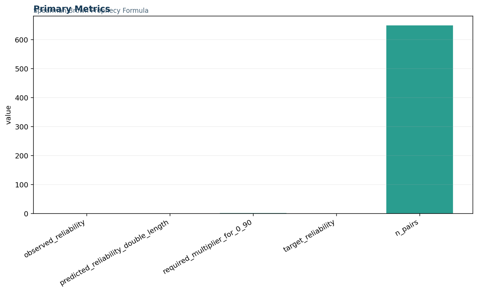
Python chart 1: primary metrics
The first figure includes observed reliability 0.864982, doubled-length prediction 0.927603, target 0.90, required multiplier 1.404845 and 649 pairs. Because the case count is hundreds of times larger than the coefficients, it dominates the shared vertical scale. The chart verifies inclusion of all metrics, while the exact values are best read from the result table.
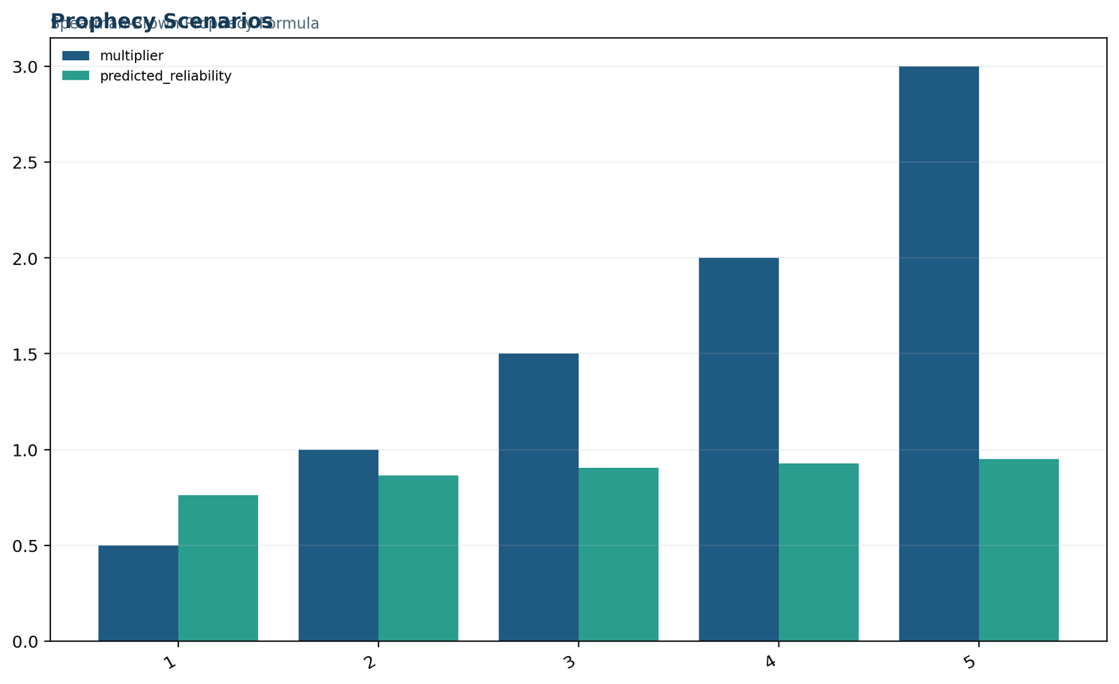
Python chart 2: prophecy scenarios
The scenario chart compares multipliers of 0.5, 1, 1.5, 2 and 3 with predicted reliability values of approximately 0.7621, 0.8650, 0.9057, 0.9276 and 0.9505. Multiplier and reliability use different units, so the bars should be interpreted as paired scenario labels rather than as directly comparable magnitudes. The reliability sequence clearly shows rapid early gains followed by diminishing returns.
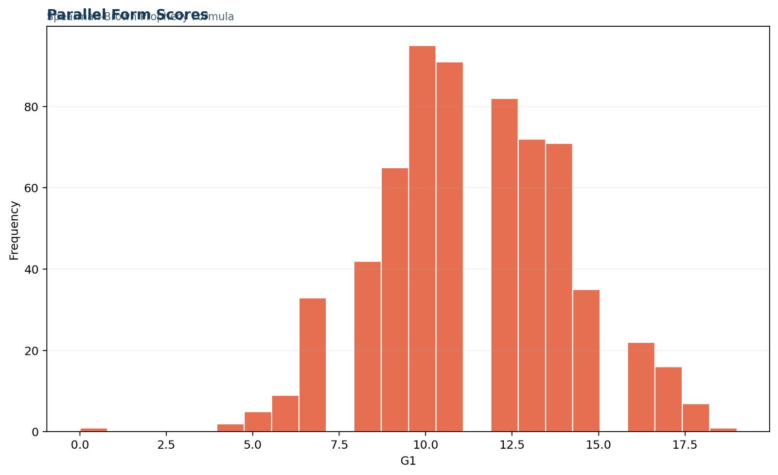
Python chart 3: parallel-score distribution
This figure displays the frequency distribution of G1. Values concentrate around 9 to 14, with a mean of 11.3991, median of 11 and range from 0 to 19. The title identifies the paired-score context, but the visible histogram is specifically the G1 distribution. Pairwise agreement is established separately by the G1-G2 correlation and the SPSS scatterplot.
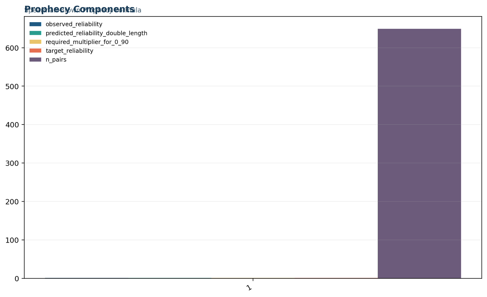
Python chart 4: prophecy components
The component figure reproduces the same five-element calculation ledger. The large n = 649 bar compresses the four coefficient-scale values near zero. This does not indicate that those values are unimportant; it reflects a unit-scale mismatch in a single-axis audit chart. The precise formula components are observed 0.864982, target 0.90, multiplier 1.404845 and doubled prediction 0.927603.
Python chart 5: verified result summary
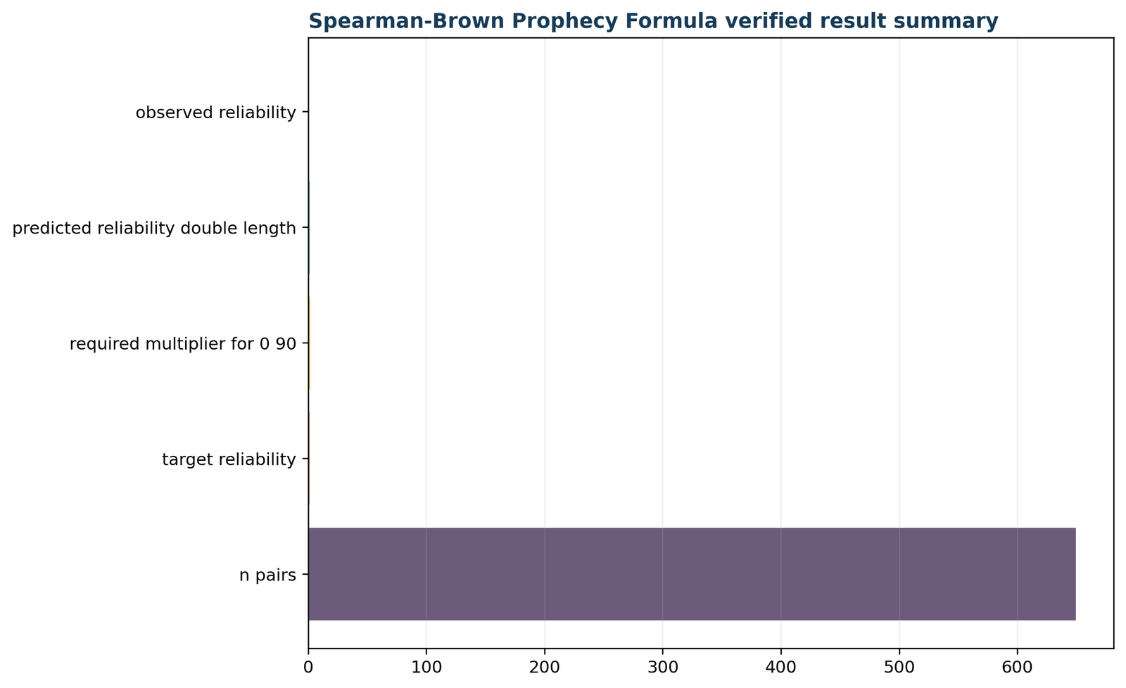
The final horizontal summary confirms the same metrics and provides a visual audit that the expected result fields were generated. The pair count again controls the horizontal axis, so coefficient bars are narrow. The important verification is numerical: Python matches the workbook values within floating-point rounding and returns a pass status for all five target metrics.
Python result ledger
What Python contributes
Python makes the Spearman Brown formula transparent by exposing the source columns, computed scenarios and verification values. It is especially useful when analysts need many targets, sensitivity curves or automated reports. The reliability prediction itself requires only basic arithmetic; the value of the transcript lies in reproducibility, input checks and a permanent audit trail.
For related implementation context, see correlation in Python and histogram interpretation.
Spearman Brown formula in R: independent verification
The R workflow reproduces the Python values and chart sequence using the same 649 paired observations.
The R analysis calculates the G1-G2 correlation with complete paired values, applies the same Spearman Brown prophecy formula, creates the same five multiplier scenarios and solves for the .90 target. Agreement with Python and Excel is exact to ordinary floating-point precision: small differences in the final decimal place arise from software representation rather than from a different statistical method.
R chart 1: primary metrics
The R primary-metrics placement reports the same core ledger: observed coefficient 0.864982, predicted double-length coefficient 0.927603, target 0.90, required multiplier 1.404845 and 649 complete pairs. The numerical agreement demonstrates that the result does not depend on a language-specific reliability package.
R chart 2: length-change scenarios
R reproduces the nonlinear reliability curve. Halving the measure predicts 0.762086; retaining the current length returns 0.864982; increasing to 1.5× predicts 0.905746; doubling predicts 0.927603; and tripling predicts 0.950542. The ordered values verify both shortening and lengthening behavior.
R chart 3: source-score distribution
The source-score figure shows the same G1 frequency pattern used by Python. Most observations lie in the central grade range, with thinner tails near the minimum and maximum. Distribution review supports data-quality assessment, but the Spearman Brown formula uses the observed correlation rather than requiring normal score distributions as a direct algebraic condition.
R chart 4: component ledger
The component ledger places coefficient inputs and pair count in one figure. As in Python, 649 determines the visible scale. The important cross-check is that R names and records every required component and that the coefficient values match the formula calculations in the workbook.
R chart 5: verified result summary
The final R placement confirms the completed metric set. The exact output records observed reliability 0.8649816303, doubled prediction 0.9276033782, required multiplier 1.4048452414, target .90 and 649 pairs. Matching values across R, Python and Excel establish computational reproducibility.
R users may apply the equation directly or use a documented classical-test-theory function. Whichever route is chosen, the report should name the starting reliability, multiplier or target, missing-data rule and whether the input is a full-test reliability or a correlation between halves. Related site resources include correlation in R and Cronbach’s alpha.
Spearman Brown formula in SPSS: output and interpretation
SPSS verifies the paired-score correlation, two-component reliability and descriptive evidence used in the prediction.
SPSS does not require the analyst to treat the prophecy calculation as a significance test. In the verified workflow, the G1-G2 correlation is estimated first, two-item reliability statistics are produced for comparison, the paired means and scatterplot are reviewed, and the exact Spearman Brown formula values are recorded as a calculation ledger.
Correlation and case processing
The Correlations table reports r = .865 for G1 and G2 with N = 649 and p < .001. The significance result tests whether the population Pearson correlation is zero under the stated model. It does not test whether the Spearman Brown prediction is correct, whether the components are parallel, or whether a doubled measure will actually achieve .928 reliability.
The reliability Case Processing Summary reports 649 valid cases and 0 excluded cases. This matches the complete-pair rule used by Python, R and Excel.
Two-item reliability comparison
SPSS reports raw Cronbach’s alpha of .927 and alpha based on standardized items of .928. The standardized value equals the equal-weight two-component Spearman-Brown coefficient calculated from r = .864982. Raw alpha is slightly lower because G1 and G2 have standard deviations of 2.745 and 2.914 rather than exactly equal variances.
The Inter-Item Correlation Matrix reports .865, and the scale statistics show a mean of 22.97, variance of 29.863 and standard deviation of 5.465 for the two-score sum.
| SPSS output block | Verified value | How to interpret it |
|---|---|---|
| Correlations | G1-G2 r = .865; N = 649; p < .001 | Supplies the observed relationship used as the prophecy input in this demonstration. |
| Case Processing Summary | 649 valid; 0 excluded | Confirms consistent case selection. |
| Reliability Statistics | Raw alpha = .927; standardized alpha = .928 | Shows the small raw-versus-standardized difference caused by unequal component variances. |
| Item Statistics | G1 mean 11.40, SD 2.745; G2 mean 11.57, SD 2.914 | Provides location and scale context. |
| Paired Samples Test | G1 − G2 = −0.171; t(648) = −2.945; p = .003 | Shows a small average change between occasions; it is not a reliability test. |
| Scatterplot | Strong positive cloud | Supports review of linear association, range and unusual observations. |
| Exact verification echo | 0.8649816303; 0.9276033782; 1.4048452414 | Reconciles SPSS with Python, R and Excel. |
Spearman Brown formula in Excel: worked workbook
The workbook exposes the direct formula, rearranged target equation, scenarios and cross-software checks.
The worked Spearman Brown formula Excel file is designed as an audit workbook rather than a single answer cell. It contains Guide, Data_Input, Working, Calculations, Diagnostics and Reporting sheets. Yellow reference cells and green formula-driven cells distinguish declared verification values from calculations linked to the 649 source rows.
Guide
Documents the statistical design, variables, source-row count, formula, target and scope of every sheet. It identifies the analysis as reliability prediction after changing length from the observed G1-G2 relationship.
Data_Input
Contains the unchanged G1 and G2 values. Keeping source columns separate from calculations preserves row lineage and makes it easier to audit missing values, sorting or accidental edits.
Working
Links each source row and calculates G2 − G1, G1×G2, G1² and G2². These columns expose the components behind correlation and paired-score checks without changing the source values.
Calculations
Uses CORREL for the observed coefficient, applies 2r/(1+r) for the double-length prediction and uses the rearranged equation for the .90 target. It compares each workbook value with an independently verified reference.
Diagnostics
States that the formula predicts reliability after a declared length change, retains 649 rows, uses G1 and G2, and should not be mistaken for an automatically generated odd-even split-half coefficient.
Reporting
Links final metrics, shows absolute differences from verified values and records agreement among Python, R, SPSS and Excel. Differences are effectively zero at the displayed precision.
For a general multiplier stored in a cell, replace 2 with the multiplier reference and use =k*r/(1+(k-1)*r). The target-length expression is =Target*(1-r)/(r*(1-Target)).
Workbook verification values
Excel interpretation
The tiny differences are ordinary binary floating-point effects, not substantive disagreements. They are far below any reporting precision used for reliability coefficients. The workbook therefore passes its cross-check while retaining full numeric traceability.
For broader spreadsheet context, see correlation in Excel and the site’s guide to confidence interval formulas when uncertainty calculations are added.
Spearman Brown formula planning scenarios: shortening, lengthening and targets
Use the same equation consistently for item counts, repeated trials, ratings and other comparable measurement units.
The Spearman Brown prophecy formula supports more than a single doubling calculation. It can estimate the reliability consequences of shortening, moderate expansion, repeated ratings, additional trials and a declared target coefficient, provided the multiplier refers to comparable units of measurement.
Length-change scenarios from the worked coefficient
| Multiplier, k | Design interpretation | Predicted reliability | Change from observed |
|---|---|---|---|
| 0.50 | Half the current amount | 0.762086 | −0.102896 |
| 1.00 | No length change | 0.864982 | 0.000000 |
| 1.50 | 50% more comparable material | 0.905746 | +0.040764 |
| 2.00 | Double the current amount | 0.927603 | +0.062622 |
| 3.00 | Triple the current amount | 0.950542 | +0.085560 |
The increments become smaller as reliability approaches 1. This diminishing-return pattern is why a very long test may impose substantial burden for only a modest additional gain.
Target-reliability scenarios
| Target reliability | Required multiplier | Practical reading |
|---|---|---|
| 0.80 | 0.624376 | The current measure could theoretically be shortened to about 62.4% of its length while retaining .80 reliability. |
| 0.85 | 0.884532 | A modest shortening is predicted to retain .85 reliability. |
| 0.90 | 1.404845 | Approximately 40.5% more comparable measurement is required. |
| 0.95 | 2.965784 | Nearly triple the current amount is required, illustrating sharply diminishing returns. |
For item counts, multiply the present number of items by the required multiplier and round upward. Then review content balance and administration constraints rather than adding items solely to satisfy an arithmetic target.
Define the unit
Items, raters, trials or occasions must be counted consistently.
Choose the target
Set reliability according to the intended decision and stakes.
Calculate k
Use the rearranged formula with unrounded coefficients.
Round operationally
Convert the multiplier into a feasible whole number of units.
Validate the revision
Pilot the new form and estimate reliability from observed scores.
Spearman Brown formula compared with related reliability methods
Choose the coefficient or model that matches the score design, error source and research question.
| Method | Primary question | Relationship to the Spearman Brown formula |
|---|---|---|
| Spearman Brown formula | How will reliability change if comparable measurement length changes? | Direct prediction or required-length calculation; also steps up equal split-half correlation. |
| Cronbach’s alpha | How consistently do multiple scored items form a composite under an alpha model? | For two standardized components, alpha equals 2r/(1+r); raw alpha can differ when variances differ. |
| Split-half reliability | How consistent are two parts of a test? | The half correlation is commonly corrected to full length with the Spearman Brown formula. |
| Guttman’s lambda family | What lower-bound reliability estimates arise from variance and covariance decompositions? | Includes alternatives such as lambda-4 for a split; not identical to the prophecy formula. |
| McDonald’s omega | How much composite-score variance is attributable to modeled common factors? | Uses a factor model rather than a simple proportional length transformation. |
| KR-20 | What is internal consistency for dichotomously scored items? | Equivalent to raw alpha for binary items; it does not directly forecast a new length unless paired with a prophecy model. |
| Test-retest reliability | Are scores stable across occasions? | Represents temporal stability; adding items may not reduce all occasion-specific error. |
| Intraclass correlation coefficient | How consistent or absolutely agreeing are repeated ratings or measurements? | Depends on an ANOVA/design model; average-measure ICCs can use a Spearman-Brown-type adjustment but require explicit ICC selection. |
| Cohen’s kappa | How much categorical agreement exists between two raters beyond chance? | Nominal/ordinal agreement method; the ordinary prophecy formula is not a substitute. |
| Weighted kappa | How much ordinal categorical agreement exists with graded disagreement? | Uses category weights and chance correction, not continuous test-length prediction. |
Why standardized alpha matches the doubled prediction
For two standardized components with correlation r, coefficient alpha is 2r/(1+r), the same algebra as the equal-half Spearman Brown correction. In this example, both equal 0.927603. The identity does not mean alpha and the Spearman Brown prophecy formula are interchangeable in every multi-item setting. Alpha uses a covariance structure across all items; the prophecy formula transforms a declared starting reliability and length ratio.
Choosing a method
Begin with the source of error. Use internal-consistency coefficients for item sampling, test-retest designs for temporal stability, inter-rater coefficients for rater variability and the Spearman Brown formula for proportional length planning under comparable measurement. Report multiple coefficients only when each addresses a clear aspect of the score’s intended interpretation.
The site’s correlation versus regression guide also helps separate association from predictive modeling.
Diagnostics, sensitivity checks and common Spearman Brown mistakes
Check the multiplier, starting coefficient, split design, comparability assumption and practical consequences before acting on the prediction.
Using the wrong multiplier
The multiplier is new length divided by old length, not the number of items added. Expanding a 40-item test to 60 items gives k = 60/40 = 1.5, not 20. Shortening 80 items to 50 gives k = 50/80 = 0.625. A wrong multiplier can produce a plausible-looking but meaningless coefficient.
Confusing half correlation with full reliability
In split-half work, the correlation between two half scores describes half-length forms. Applying k = 2 estimates whole-test reliability. Do not enter a whole-test alpha into the equal-half correction and then call the result corrected split-half reliability unless the design truly represents doubling the same measurement unit.
Confusing Spearman-Brown with Spearman rho
Spearman rank correlation is an association statistic. The shared name “Spearman” does not make rank correlation the default input for the prophecy formula. Equal-half correction normally uses Pearson correlation between continuous half scores unless a different model is substantively justified.
Assuming all added items are equally useful
The formula treats additional material as comparable on average. Poorly targeted or redundant items may add administration time without the predicted information. A revised form should be piloted, analyzed and reviewed for content coverage.
Treating a p-value as reliability evidence
A highly significant correlation can occur with modest magnitude in a large sample. Reliability interpretation depends primarily on the coefficient and measurement design, not on whether the correlation differs from zero. The prophecy calculation has no automatic p-value.
Ignoring unequal halves
The familiar 2r/(1+r) form assumes equal-length halves. SPSS can report equal- and unequal-length Spearman-Brown results in a split-half model. When halves differ in length or variance, document the selected estimator rather than forcing the equal-half shortcut.
Range restriction
A homogeneous sample can suppress correlations and lower the starting coefficient, while a broad sample can increase it. A prophecy based on one population may not transfer to another.
Local dependence
Near-duplicate items can inflate internal consistency without proportionally increasing meaningful construct coverage. A longer test can be reliable yet inefficient or narrow.
Changing construct
Adding a new domain may change the total score’s meaning. The resulting test is not merely a longer version of the original, so the prophecy model may be inappropriate.
How to report the Spearman Brown formula in APA style
A complete report names the score, starting coefficient, multiplier or target, prediction, sample and assumptions.
APA-style worked example
A Spearman-Brown prophecy calculation was used to estimate reliability after changing the amount of comparable measurement. First-period grade (G1) and second-period grade (G2) were available for 649 complete cases and were strongly correlated, r = .865. Using this coefficient as the starting parallel-score estimate, doubling the measurement length was predicted to increase reliability to .928, ρSB = 2(.865)/[1 + .865]. The rearranged Spearman-Brown formula indicated that a length multiplier of 1.405, equivalent to an increase of approximately 40.5%, would be required to reach a target reliability of .90. These values are conditional predictions that assume the added measurement units have properties comparable to those of the current measure.
Minimum reporting checklist
Alternative concise wording
Split-half application: “The correlation between the two equal-length halves was .865. The Spearman-Brown corrected reliability for the full test was .928.”
Length-planning application: “Assuming newly added items are comparable to current items, increasing test length by a factor of 1.405 is predicted to raise reliability from .865 to .90.”
Shortening application: “Reducing the measure to half its current length is predicted to lower reliability from .865 to .762.”
Use leading-zero conventions required by the publication style. In APA prose, correlations and reliability coefficients are commonly written without a leading zero because their theoretical range does not exceed 1.
Spearman Brown formula PDF, SPSS and Excel downloads
Open the exact Python, R, SPSS and worked Excel files used throughout the analysis.
All four Spearman Brown formula downloads refer to the same 649-pair calculation. Python and R retain exact values and scenario tables, SPSS supplies the correlation, reliability and paired-score output, and Excel exposes the complete formula chain and cross-software ledger.
Spearman Brown formula verification sources and software records
The supplied analysis files provide a complete cross-platform audit of the worked values.
The numerical values in this Spearman Brown formula guide were checked against the supplied Python script, R script, SPSS output and worked Excel workbook. All four implementations use the same 649 paired observations and reconcile the observed coefficient, double-length prediction and target multiplier.
Python calculation record
The supplied Python analysis reads G1 and G2, calculates Pearson r = 0.8649816303, applies the prophecy equation for several multipliers and verifies the required multiplier for a .90 target.
R calculation record
The supplied R analysis independently calculates the same coefficient and scenario table, then produces a matched report and verification summary.
SPSS and Excel audit
The SPSS output confirms 649 valid cases, r = .865, standardized two-component reliability of .928 and paired-score descriptives. The Excel workbook exposes each formula and cross-software check.
Spearman Brown formula FAQs
Answers to the most important calculation, split-half, interpretation and planning questions.
These Spearman Brown formula FAQs address the questions most likely to cause calculation or interpretation errors: the difference between the prophecy formula and rank correlation, how to define the multiplier, how split-half correction works, why coefficients show diminishing returns, and why revised scores must still be tested empirically.
What is the Spearman Brown formula?
The Spearman Brown formula predicts how reliability changes when the amount of comparable measurement is lengthened or shortened. It can also correct the correlation between two equal test halves to estimate whole-test split-half reliability. The prediction form is ρnew = kρold/[1 + (k − 1)ρold].
What is the Spearman Brown prophecy formula used for?
It is used for test-length planning, survey shortening, trial-number planning, equal split-half correction and target-reliability calculations. It estimates a future coefficient under the assumption that added or retained measurement units have properties comparable to the current units.
Why is it called a prophecy formula?
The term “prophecy” emphasizes that the equation predicts a reliability value for a test length that may not yet exist. The output is conditional rather than observed. After the revised measure is built, its reliability should be estimated from actual data.
How do I calculate the Spearman Brown formula?
Multiply current reliability by the length multiplier. Divide that product by 1 plus the product of current reliability and one less than the multiplier. For ρ = .864982 and k = 2, the result is .927603.
What does k mean in the Spearman Brown formula?
k is new length divided by current length. A 60-item version of a 40-item test has k = 1.5. A 30-item version of the same 40-item test has k = .75. It is a ratio, not the raw number of items added or removed.
How is the formula used for split-half reliability?
Correlate the two equal-length half scores, then set k = 2 because combining them restores the full length. The corrected coefficient is 2r/(1+r). The halves should be designed to be comparable in content, difficulty and variance.
Is the Spearman Brown formula the same as Spearman correlation?
No. Spearman rank correlation measures monotonic association between two ranked or ordinal variables. The Spearman Brown formula is a reliability prediction equation. The procedures share Charles Spearman’s name but answer different questions.
What is the predicted reliability if the worked measure is doubled?
Using observed r = 0.8649816303 and k = 2, the predicted reliability is 0.9276033782. Rounded to three decimals, the result is .928.
How much longer must the measure be to reach reliability .90?
The rearranged formula gives k = 1.4048452414. That corresponds to an increase of about 40.4845%. Multiply the current item count by 1.404845 and round upward for a practical whole-item plan.
Can the formula predict reliability after shortening?
Yes. Use a multiplier between 0 and 1. Halving the worked measure, k = .5, predicts reliability of 0.762086. The prediction assumes the removed units have average properties similar to the units retained.
Does doubling the test double reliability?
No. Reliability is bounded and changes nonlinearly. In the example, doubling length raises the coefficient from .865 to .928, not to 1.730. Gains become smaller as reliability approaches 1.
Does the Spearman Brown formula have a p-value?
No. The equation is a deterministic transformation of an input coefficient and a length ratio. A p-value shown for the starting correlation tests a separate null hypothesis. Uncertainty for the predicted coefficient requires an explicitly chosen confidence-interval or bootstrap method.
Related statistical guides
Continue with the reliability, correlation and measurement topics most closely connected to the Spearman Brown formula.