
Multilevel Regression: Formula, Interpretation, SPSS, Python, R and Excel Guide
A complete worked analysis of 649 students nested in GP and MS, including centered Python estimates, raw-unit R estimates, an SPSS execution audit, Excel guidance, coefficient interpretation, predictions, residual checks, and the limits created by having only two level-2 units.
Multilevel Regression Model Overview
What Multilevel Regression Is
Multilevel Regression is a regression framework for data in which observations are grouped inside larger units. Students may be nested in schools, patients in hospitals, employees in companies, repeated measurements in people, or survey respondents in regions. The model keeps the familiar fixed-effect regression equation but adds one or more random effects so that records from the same cluster are not treated as fully independent.
The worked Multilevel Regression analysis uses final grade G3 as the outcome and school as the level-2 grouping variable. Each student is a level-1 observation. The model estimates the adjusted relationships of prior grades, study time, failures, absences, age, sex, address, and family size with G3, while allowing GP and MS to have separate conditional intercept deviations.
The Research Question Answered
The central Multilevel Regression question is not merely whether GP and MS have different raw average grades. It asks how much of the remaining variation in final grade is attributable to school after accounting for measured student characteristics, and which student-level coefficients remain supported when the common school context is represented in the covariance structure.
That question has two connected parts. The fixed part estimates average slopes such as the expected change in G3 for a one-point increase in G2. The random part estimates the remaining school-to-school intercept variance. The intraclass correlation coefficient, or ICC, converts the two variance components into the proportion of modeled variance associated with the grouping level.
When Multilevel Regression Should Be Used
Multilevel Regression is appropriate when the sampling, design, or data-generating process creates meaningful clusters and when observations within a cluster may be more alike than observations from different clusters. A useful analysis normally has a defensible level-2 unit, enough clusters to estimate between-cluster variation, and a research question that concerns both individual-level relationships and contextual dependence.
The method is not justified merely because a grouping column exists. It should not be used as a decorative alternative to ordinary least squares. The cluster must have scientific meaning, and the random structure must correspond to the dependence expected in the data. In this example, school is meaningful, but the presence of only two schools places a severe limit on the precision and generalizability of the random-effect variance.
Why Ordinary Regression Is Not the Same Analysis
Ordinary linear regression assumes independent residuals after conditioning on the predictors. Multilevel Regression relaxes that assumption by giving students from the same school a shared random intercept. Ignoring clustering can make standard errors too small when the ICC is appreciable, and it prevents direct estimation of the school-level variance component.
However, the adjusted ICC in this worked analysis is extremely small. Python estimates 0.000568 and R estimates 0.004918. Therefore, the fitted fixed slopes and prediction errors are close to their fixed-only counterparts. That empirical result does not make the multilevel question invalid; it shows that the measured predictors absorb nearly all residual school-intercept separation in these two schools.
How the Model Operates Conceptually
For student i in school j, Multilevel Regression combines a population intercept, fixed slopes, a school-specific random intercept u0j, and a student residual. The random intercept shifts every fitted value in a school by the same amount. The saved models do not include random slopes, so the effects of G1, G2, and the other predictors are assumed constant across GP and MS.
The variance of u0j is the between-school variance. The variance of the student residual is the within-school variance. Their ratio produces the ICC. Conditional predictions include the estimated school intercept, whereas population-level predictions set the random effect to zero. Those two prediction targets should not be confused.
How Coefficients and Effects Are Interpreted
Each fixed coefficient in Multilevel Regression is interpreted conditionally: it is the expected outcome difference associated with a one-unit predictor difference, holding the other fixed predictors and the school intercept constant. A categorical coefficient compares a category with its stated reference group. A random intercept is not a causal school effect; it is a fitted residual deviation under the specified model.
Python grand-mean centers six numeric predictors, so its slopes remain in original units but its intercept refers to average numeric values. R leaves those predictors uncentered, producing nearly identical slopes but a very different intercept. SPSS standardizes ten numeric variables, so its coefficients represent one-standard-deviation changes and cannot be compared directly with the raw-unit Python and R coefficients.
How Multilevel Regression Differs from Related Methods
Multilevel Regression, mixed-effects regression, hierarchical linear modeling, and random-effects regression often describe overlapping families of models. The distinguishing issue is the random structure, not the label. A fixed-effects model with a dummy for each school controls for observed schools but does not estimate a variance distribution for schools. A generalized estimating equation models population-average effects and within-cluster correlation without estimating random intercepts in the same way.
A repeated-measures model is also multilevel when occasions are nested within people, but this dataset has one row per student rather than repeated grades per student. A random-slope model would allow the G2 effect to vary by school; the saved analysis has only random intercepts and cannot answer that question.
Supported Variables, Assumptions, Advantages and Limits
Multilevel Regression can include continuous, binary, categorical, interaction, polynomial, and cluster-level predictors, provided they are coded and interpreted correctly. The model assumes an appropriate grouping structure, independent clusters, a correctly specified mean equation, a defensible random-effect distribution, and residual behavior compatible with the selected outcome family.
Its advantages are explicit variance decomposition, cluster-aware uncertainty, flexible random effects, and conditional prediction. Its limitations include dependence on the number of clusters, sensitivity to singular or boundary fits, more complex interpretation, and the need to separate within-cluster from between-cluster information. Those limitations are decisive here because 649 rows do not compensate for having only two schools.
Connection to the Worked Dataset
The worked Multilevel Regression package is best understood as a careful two-school audit rather than a broad school-population study. GP has 423 students and MS has 226. Their unadjusted mean final grades differ by about 1.926 points, but the R empty-model ICC of 0.159464 falls to 0.004918 after prior grades and other student predictors enter. Python reaches the same qualitative conclusion with an adjusted ICC of 0.000568.
The strongest replicated fixed effects are G1, G2, and failures. Python reports additional significance for sex and absences, but its covariance calculation is partly singular and the address standard error is missing. R supplies finite uncertainty and does not support sex or absences at the .05 level. SPSS does not provide a valid mixed model because both saved MIXED commands stop at an invalid FIT print option.
For a broader foundation, compare this framework with
Ordinary Least Squares Regression,
Mixed Effects Regression, and
Hierarchical Linear Model.
These guides clarify what changes when clustered observations require both fixed and random components.
Quick Answer
Verified Answer from the Saved Multilevel Regression Runs
Stable fixed-effect evidence
G1: about +0.135 to +0.138 grade points per pointG2: about +0.880 to +0.881 per point- Failures: about -0.223 per additional failure
Random-effect conclusion
- R empty-model ICC: 0.159464
- R adjusted ICC: 0.004918
- Python adjusted ICC: 0.000568
The verified Multilevel Regression conclusion is that measured student characteristics, especially prior grades, explain almost all adjusted school-intercept separation in these records. R estimates between-school variance of 0.007738 and residual variance of 1.565638. Python estimates between-school variance of 0.000878 and residual variance of 1.543595.
The strongest replicated slopes are positive for G1 and G2 and negative for failures. Python also labels male sex and absences significant, but the same two terms do not reach .05 in R. Because Python has a singular covariance problem and no standard error for address, the cross-software evidence supports the narrower set of G1, G2, and failures.
MIXED commands stop because FIT is not accepted in the /PRINT subcommand. No SPSS mixed-model ICC, random effect, or variance component should be reported.Table of Contents
- Quick Answer
- Why This Analysis Needs Multilevel Regression
- How Multilevel Regression Works
- Variables Used, Coding and Standardization
- Multilevel Regression Results
- Python Charts and Explanations
- R Charts and Explanations
- Multilevel Regression Coefficients
- Predictions, Effects and Model Meaning
- Multilevel Regression Assumptions and Diagnostics
- Multilevel Regression in Python, R, SPSS and Excel
- Code: Expand Only the Software You Need
- Advanced Multilevel Regression Topics
- APA-Style Reporting
- Publication Checklist
- Downloads and Chart Resources
- Related Salar Cafe Guides
- Frequently Asked Questions
- Multilevel Regression Conclusion
Why This Analysis Needs Multilevel Regression
The Nesting Problem
Multilevel Regression is needed because students who attend the same school share conditions that may affect grades: policies, teachers, calendars, peer composition, and unmeasured institutional features. A random school intercept represents the possibility that otherwise comparable students from GP and MS have different baseline outcomes.
The raw data show a clear group contrast. GP has 423 students with mean G3 12.576832, whereas MS has 226 students with mean 10.650442. The unadjusted difference is approximately 1.926390 points. MS also has a larger standard deviation, 3.833991 versus 2.625636 in GP. These descriptive differences justify examining school structure, but they do not prove a school effect.
Why the Raw School Gap Is Not the Model Result
The Multilevel Regression random intercept is conditional on the fixed predictors. GP and MS may enroll students with different previous grades, failure histories, attendance records, or demographic characteristics. Once those variables enter the equation, the school intercept represents only the residual baseline contrast left after adjustment.
That distinction is visible in R. The empty model estimates ICC 0.159464, indicating noticeable unconditional clustering. The full model estimates ICC 0.004918. The decrease does not mean the original school difference was imaginary. It means the entered student variables account for almost all of the between-school component present in the intercept-only model.
The Important Limitation: Only Two Schools
A valid reason to consider Multilevel Regression is not the same as adequate information for every multilevel parameter. The 649 student records provide substantial information about student-level slopes, but the between-school variance is informed by only two level-2 units. Estimating a population distribution of school effects from GP and MS alone is intrinsically fragile.
The random-intercept analysis therefore answers a narrow, useful question: after adjustment, how much conditional baseline separation remains between these two observed schools under the fitted model? It does not support a general estimate of school-to-school variability across a wider education system.
Before interpreting the adjusted school component, use
Descriptive Statistics
to summarize the raw GP–MS contrast and
Effect Size
to distinguish the size of an observed difference from its statistical significance.
How Multilevel Regression Works
Random-Intercept Formula
In the worked Multilevel Regression model, i indexes students and j indexes schools. The fixed coefficients are shared across GP and MS. The school random intercept u0j shifts the complete regression line upward or downward for a school, and the residual εij captures the remaining student-level deviation.
Students are level 1 and school is level 2. Confirm that one row belongs to one school and that school is the intended source of shared dependence.
Estimate the average slopes together with the school-intercept variance and the within-school residual variance.
Calculate the ICC, inspect boundary behavior, compare valid software outputs, and avoid relying on unstable Wald tests.
Variance Components and ICC
The Multilevel Regression quantity τ00 is the variance of school intercepts, and σ2 is the within-school residual variance. The ICC is the model-implied correlation between two otherwise comparable students from the same school under a random-intercept specification.
R’s empty model gives τ00 = 1.822876 and σ2 = 9.608405, producing ICC 0.159464. After the fixed predictors enter, R gives τ00 = 0.007738 and σ2 = 1.565638, producing ICC 0.004918. Python’s adjusted estimates are 0.000878 and 1.543595, producing ICC 0.000568.
Centered and Uncentered Equations
Python grand-mean centers G1, G2, study time, failures, absences, and age before fitting Multilevel Regression. For a numeric predictor x, the centered value is x minus its sample mean. This transformation does not change the unit or the slope in the same additive model; it changes the intercept.
R uses the original numeric scales. That is why the Python and R slopes are close while the intercepts differ sharply. Python’s intercept is meaningful for the reference categories at average numeric values. R’s raw intercept corresponds to numeric predictors equal to zero, which is outside or near the edge of the meaningful range for several variables.
ML, REML, and the Saved Software Runs
Python fits the saved Multilevel Regression model by maximum likelihood, whereas R uses restricted maximum likelihood. ML estimates fixed effects and variance components jointly and is commonly used when comparing models with different fixed effects. REML adjusts the variance estimation for the loss of degrees of freedom caused by estimating fixed effects and is often preferred for final variance estimates when the fixed structure is held constant.
Because the saved Python and R models differ in centering, optimizer implementation, covariance calculation, and ML versus REML, their likelihoods and information criteria should not be pooled or ranked against each other. The proper cross-software audit compares the substantive slopes, fitted values, residual summaries, and variance conclusions while preserving each run’s estimation context.
What the Model Does Not Estimate
The saved Multilevel Regression specification has no school-level predictor, no random slope, no cross-level interaction, and no separate residual variance by school. It cannot determine whether the G2 slope differs between GP and MS, whether school-level resources explain the intercept difference, or whether within-school variance should differ across schools.
The variance partition connects directly to the
Intraclass Correlation Coefficient.
Researchers interested in population-average rather than cluster-specific effects should also compare
Generalized Estimating Equations
with the conditional interpretation used here.
Variables Used, Coding and Standardization
Data Dictionary and Coding
The worked Multilevel Regression analysis retains all 649 records because the selected Python and R variables are complete. GP contributes 423 students and MS contributes 226. The original file has 33 columns, but the mixed equation uses a focused student-level subset plus school as the grouping variable.
| Variable | Role | Coding or meaning | Model treatment |
|---|---|---|---|
G3 | Level-1 outcome | Final grade; observed range 0 to 19 | Modeled as a continuous Gaussian response in Python and R |
school | Level-2 grouping variable | GP or MS | Defines the random intercept |
G1 | Level-1 predictor | First-period grade | Centered in Python; raw in R; standardized in SPSS |
G2 | Level-1 predictor | Second-period grade | Centered in Python; raw in R; standardized in SPSS |
studytime | Level-1 predictor | Ordered study-time code | Entered numerically |
failures | Level-1 predictor | Prior class failures | Entered numerically |
absences | Level-1 predictor | Recorded absences | Entered numerically |
age | Level-1 predictor | Student age | Entered numerically |
sex | Level-1 factor | Female reference; male comparison | Unchanged by centering |
address | Level-1 factor | Rural reference; urban comparison | Python standard error is unavailable |
famsize | Level-1 factor | GT3 reference; LE3 comparison | Included in Python and R |
Outcome Distribution by School
| Quantity | GP | MS | Overall or interpretation |
|---|---|---|---|
| n | 423 | 226 | 649 |
Mean G3 | 12.576832 | 10.650442 | 11.906009 overall |
SD G3 | 2.625636 | 3.833991 | 3.230656 overall |
| Mean 95% CI | 12.3266 to 12.8271 | 10.1506 to 11.1503 | Descriptive intervals |
| Observed range | 0 to 19 | 0 to 19 | Bounded integer-valued outcome |
The raw mean contrast is important context, but Multilevel Regression does not treat it as an adjusted school effect. The fitted random intercept is estimated after the student predictors enter, and its magnitude becomes much smaller than the observed mean difference.
Centering and Standardization Are Different
Python subtracts the full-sample mean from six numeric variables. The means are approximately 11.3991 for G1, 11.5701 for G2, 1.9307 for study time, 0.2219 for failures, 3.6595 for absences, and 16.7442 for age. Centering produces zero-mean columns but preserves original units.
SPSS converts ten numeric predictors to z scores. Its coefficients describe a one-standard-deviation difference rather than a one-unit difference. A valid Multilevel Regression interpretation must therefore identify the predictor scale before comparing coefficient magnitudes across software.
Variable screening should also include
Frequency Distribution
checks for categorical predictors and
Multiple Linear Regression
coding principles for reference categories, continuous slopes, and interaction-ready predictors.
Multilevel Regression Results
Python Maximum-Likelihood Multilevel Regression
The Python full model converges with log likelihood -1061.929422, AIC 2147.858844, and BIC 2201.564036. The estimated school-intercept variance is 0.000878, the within-school residual variance is 1.543595, and the resulting ICC is 0.000568. The empirical school deviations are approximately +0.009654 for GP and -0.009654 for MS.
| Centered Python term | B | SE | z | p | 95% CI |
|---|---|---|---|---|---|
| Intercept | 11.867178 | 0.094435 | 125.6656 | < .001 | 11.682090 to 12.052267 |
| Male vs female | -0.192699 | 0.086791 | -2.2203 | .0264 | -0.362807 to -0.022591 |
| Urban vs rural | 0.140931 | Not available | Not available | Not available | Not available |
| LE3 vs GT3 family size | 0.056545 | 0.104028 | 0.5436 | .5867 | -0.147347 to 0.260437 |
Centered G1 | 0.137545 | 0.032260 | 4.2637 | < .001 | 0.074317 to 0.200774 |
Centered G2 | 0.881011 | 0.033664 | 26.1708 | < .001 | 0.815031 to 0.946991 |
| Centered study time | 0.070687 | 0.056573 | 1.2495 | .2115 | -0.040193 to 0.181568 |
| Centered failures | -0.222574 | 0.094297 | -2.3603 | .0183 | -0.407393 to -0.037755 |
| Centered absences | 0.020646 | 0.005444 | 3.7921 | < .001 | 0.009975 to 0.031317 |
| Centered age | 0.019277 | 0.041698 | 0.4623 | .6439 | -0.062450 to 0.101003 |
At face value, the Python Multilevel Regression run supports male sex, G1, G2, failures, and absences. The address row cannot be tested because its standard error, test statistic, p-value, and interval are unavailable. The missing uncertainty is direct evidence that the covariance calculation is not fully regular.
Why the Python Wald Tests Need Caution
The Python and R point estimates for sex and absences are similar, but their standard errors differ. Python gives sex SE 0.086791 and absences SE 0.005444. R gives 0.103655 and 0.011044. Those differences move both terms across the .05 threshold. A responsible Multilevel Regression synthesis should not select whichever software produces the smaller p-value.
| Term | Python result | R result | Evidence assessment |
|---|---|---|---|
| Male vs female | B = -0.192699; SE = 0.086791; p = .0264 | B = -0.201066; SE = 0.103655; p = .0528 | Direction agrees; threshold conclusion does not replicate |
| Absences | B = 0.020646; SE = 0.005444; p < .001 | B = 0.019206; SE = 0.011044; p = .0825 | Point estimate agrees; uncertainty does not |
| Urban vs rural | B = 0.140931; SE unavailable | B = 0.119674; SE = 0.112052; p = .2859 | Python cannot support an inferential claim |
With only two schools and a near-zero random variance, the likelihood surface is close to a boundary. The Hessian or inverse information matrix can become unstable, causing missing or overly optimistic standard errors. The most defensible fixed-effect conclusion is therefore the set that replicates across the valid mixed outputs: G1, G2, and failures.
R Restricted-Likelihood Multilevel Regression
R fits the raw-unit equation by REML and reports full-model log likelihood -1082.550328, AIC 2189.100656, BIC 2242.619510, and residual SD 1.251255. The estimated school-intercept variance is 0.007738, residual variance is 1.565638, and adjusted ICC is 0.004918. The conditional school deviations are +0.044945 for GP and -0.044945 for MS.
| R term | B | SE | p | 95% CI | Result |
|---|---|---|---|---|---|
G1 | 0.134985 | 0.036691 | < .001 | 0.062935 to 0.207035 | Supported positive slope |
G2 | 0.880381 | 0.034162 | < .001 | 0.813298 to 0.947464 | Supported positive slope |
| Study time | 0.066619 | 0.063090 | .2914 | -0.057272 to 0.190509 | Interval crosses zero |
| Failures | -0.222767 | 0.094977 | .0193 | -0.409272 to -0.036262 | Supported negative slope |
| Absences | 0.019206 | 0.011044 | .0825 | -0.002480 to 0.040892 | Uncertain positive estimate |
| Age | 0.020996 | 0.043527 | .6297 | -0.064478 to 0.106470 | Interval crosses zero |
| Male vs female | -0.201066 | 0.103655 | .0528 | -0.404611 to 0.002480 | Borderline; interval includes zero |
| Urban vs rural | 0.119674 | 0.112052 | .2859 | -0.100361 to 0.339709 | Interval crosses zero |
| LE3 vs GT3 | 0.060922 | 0.108748 | .5755 | -0.152625 to 0.274469 | Interval crosses zero |
The R Multilevel Regression output provides finite standard errors and confidence intervals for every fixed term. It supports positive G1 and G2 slopes and a negative failures slope. The sex interval just crosses zero, and absences remains positive but uncertain.
Empty-Model and Full-Model Variance Decomposition
| Saved model | Between-school variance | Residual variance | ICC | Interpretation |
|---|---|---|---|---|
| R empty model, REML | 1.822876 | 9.608405 | 0.159464 | Noticeable unconditional school clustering |
| R full model, REML | 0.007738 | 1.565638 | 0.004918 | Nearly all remaining variance is within schools |
| Python full model, ML | 0.000878 | 1.543595 | 0.000568 | Boundary-adjacent adjusted school variance |
| Python empty model, ML | 0.000000 | 9.578795 | 0.000000 | Boundary solution; do not use a regular likelihood-ratio test |
The most informative Multilevel Regression change is the R reduction from ICC 0.159464 to 0.004918. The covariates do not merely improve prediction; they explain the composition associated with the original school mean difference. The adjusted random intercepts are tiny relative to the 0-to-19 observed outcome range and residual SD near 1.25.
SPSS: Valid OLS Comparison, Failed MIXED Commands
The saved SPSS file successfully runs a broader standardized OLS model with R = .924, R² = .854, adjusted R² = .850, and standard error of estimate 1.251. Its omnibus result is F(17, 631) = 217.194, p < .001. These are fixed-only statistics, not Multilevel Regression estimates.
| SPSS OLS term | B on entered scale | SE | p | 95% CI |
|---|---|---|---|---|
| Constant | 11.513 | 0.222 | < .001 | 11.077 to 11.949 |
Standardized G1 | 0.375 | 0.101 | < .001 | 0.176 to 0.574 |
Standardized G2 | 2.557 | 0.100 | < .001 | 2.360 to 2.753 |
| Standardized study time | 0.051 | 0.053 | .337 | -0.053 to 0.156 |
| Standardized failures | -0.129 | 0.057 | .024 | -0.242 to -0.017 |
| Standardized absences | 0.088 | 0.051 | .086 | -0.012 to 0.188 |
| Male indicator | -0.168 | 0.108 | .118 | -0.380 to 0.043 |
| Urban indicator | 0.221 | 0.116 | .058 | -0.008 to 0.449 |
Both SPSS MIXED commands contain /PRINT=SOLUTION TESTCOV FIT. The Viewer states that FIT is unrecognized and stops execution. The requested prediction variables are never created. Consequently, the SPSS file contains no valid multilevel coefficient solution, covariance parameter, ICC, random intercept, conditional prediction, or mixed-model residual.
When software packages return similar coefficients but different significance decisions, interpret the
Standard Error,
Confidence Interval, and
P-Value
together rather than selecting the smallest reported probability.
Python Charts and Explanations
Each Python chart is interpreted with the same four-part reading sequence: Pattern, Key Values, Interpretation, and Why It Matters. The charts support the numerical Multilevel Regression tables but do not replace the coefficient and covariance audit.
Python Chart 1: Outcome Distribution for Final Grade
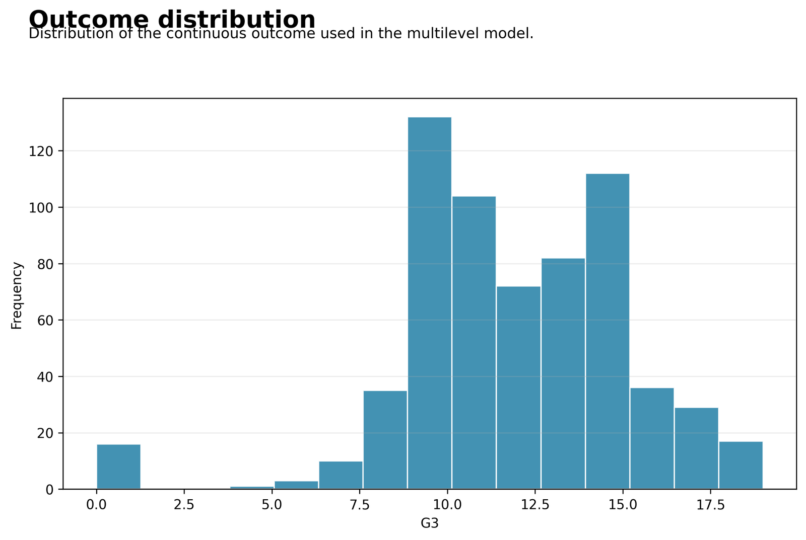
Most final grades fall in the middle and upper-middle part of the scale, while a visible low-end group includes zero grades. The discrete outcome produces bars at integer values rather than a smooth continuous shape.
The dataset contains 649 students, the overall mean is 11.906009, the standard deviation is 3.230656, and the observed range is 0 to 19.
The Gaussian Multilevel Regression model can still estimate an average linear relationship, but the bounded integer response and low-end tail should be remembered when interpreting normal-residual diagnostics.
The outcome chart establishes the response scale before coefficients or variance components are interpreted. It also explains why the most extreme negative residuals come from students with very low observed grades.
Python Chart 2: Mean Final Grade by School
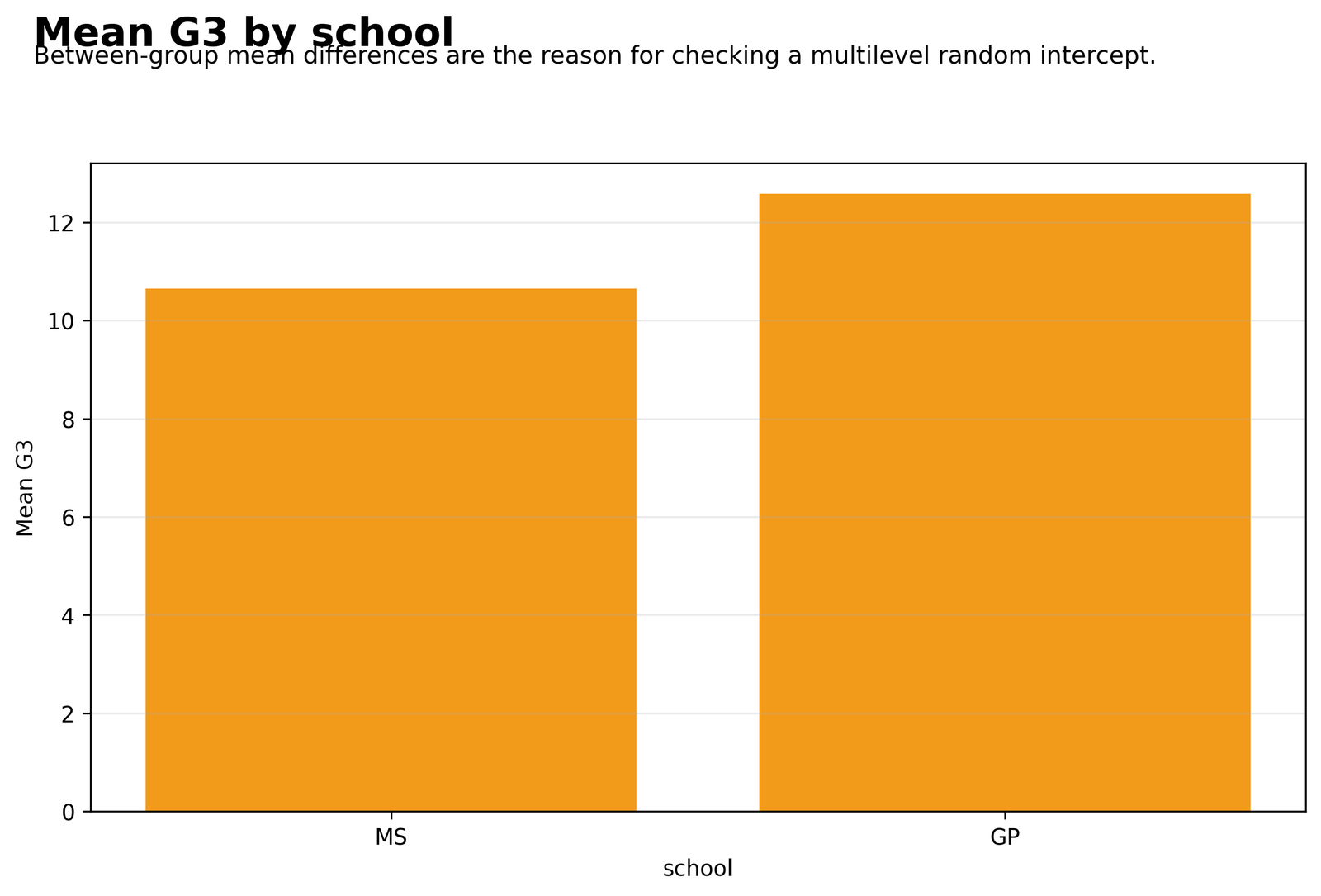
GP has the taller mean bar, and the descriptive gap is visibly larger than the adjusted random-intercept difference in either mixed model.
GP mean G3 is 12.576832 for 423 students. MS mean G3 is 10.650442 for 226 students. The raw difference is about 1.926390 points.
The bars summarize unadjusted composition. They do not hold G1, G2, failures, attendance, or other predictors constant, so they are not the conditional school effect from Multilevel Regression.
This contrast makes the empty-model ICC meaningful and shows why the adjusted ICC should be interpreted as the variance left after student characteristics enter.
Python Chart 3: Final-Grade Boxplots by School
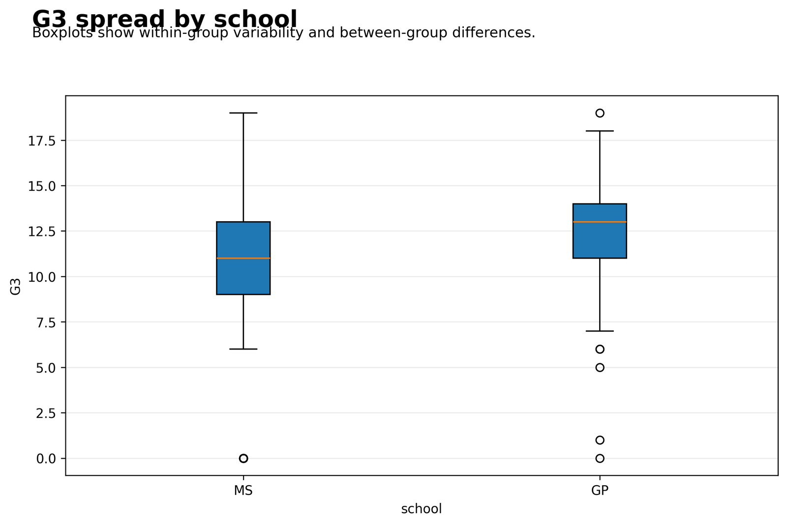
The two schools overlap across much of the grade scale. MS has a lower central location and wider spread, while GP shows several low observations, including zeros.
GP has SD 2.625636 and MS has SD 3.833991. Both schools span observed grades from 0 to 19.
The boxplots show that a two-bar mean comparison hides substantial within-school variation. The one-variance Multilevel Regression model also assumes a common residual variance despite the different raw spreads.
Unequal raw spread and low-end cases can affect residual assumptions even when the fitted school-intercept variance is tiny.
Python Chart 4: Python Fixed Effects and Confidence Intervals
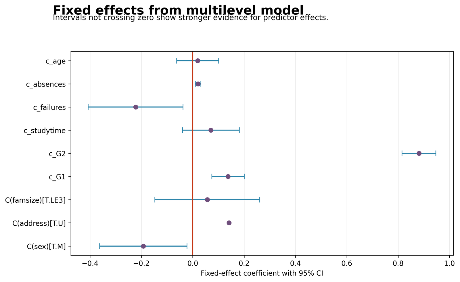
The G2 estimate is the dominant positive fixed slope. G1 is positive and failures is negative. The address point lacks an interval, visibly exposing the covariance problem.
Python estimates G2 at 0.881011, G1 at 0.137545, failures at -0.222574, male sex at -0.192699, and absences at 0.020646. The urban-address standard error is unavailable.
The graph represents the Python covariance calculation only. Because sex and absences do not replicate at .05 in R, their plotted intervals should not be treated as stable Multilevel Regression evidence.
The missing address interval is not a cosmetic omission. It is a warning that the Hessian or covariance matrix is singular or nearly singular.
Python Chart 5: Observed Versus Fitted Values
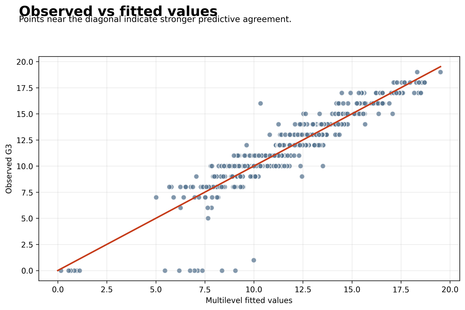
Most points follow the diagonal through the central grade range. Horizontal bands appear because observed G3 is integer-valued, and several zero-grade observations lie far below their fitted values.
Python fitted values range from 0.163407 to 19.512157. In-sample RMSE is 1.242212 and MAE is 0.778943.
Prior grades give Multilevel Regression strong in-sample predictive alignment, but the plot also shows systematic difficulty with unusual low outcomes. A high overall fit does not eliminate large individual errors.
The central cloud explains the high fixed-only R², while the low-end deviations explain the long negative residual tail.
Python Chart 6: Residuals Versus Fitted Values
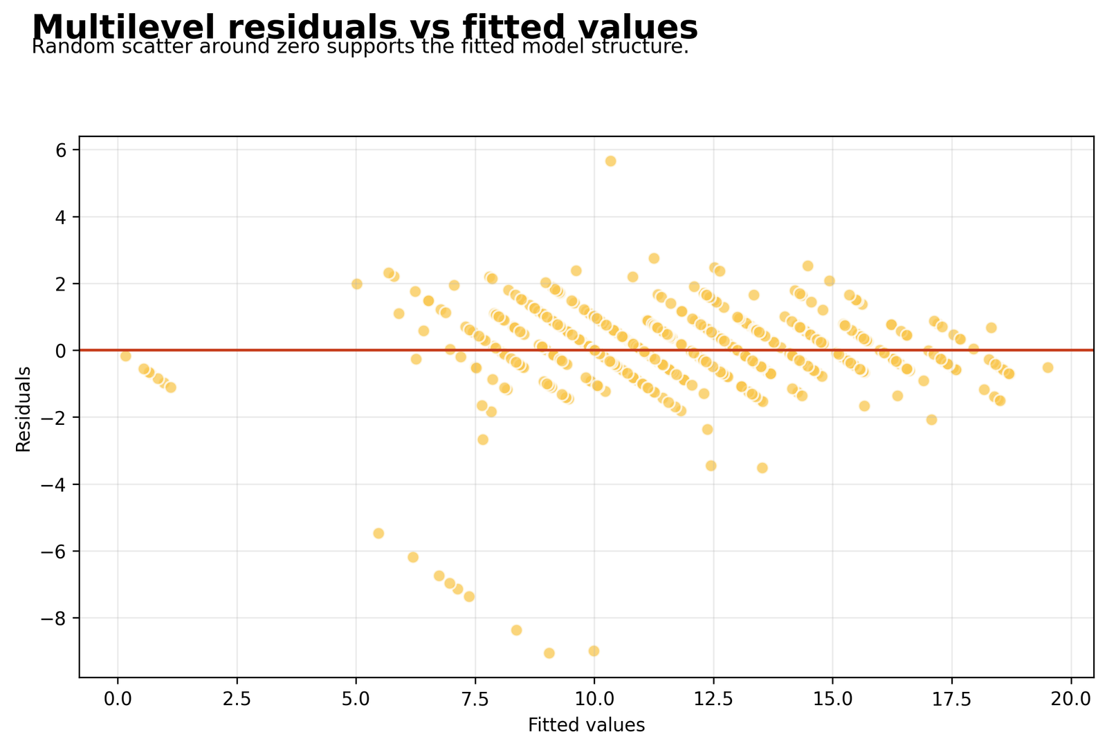
Diagonal stripes descend with slope -1 because each integer outcome forms a line as fitted values vary. The main cloud is centered near zero, but the negative tail is longer than the positive tail.
Python raw residuals range from -9.049531 to 5.664255 and have median -0.023335. The fitted values average 11.906009.
The Multilevel Regression residual pattern is not cleanly normal. The low-grade overpredictions create strong negative outliers, and the bounded response contributes to the striped geometry.
The residual plot is more informative than a single RMSE because it reveals where the model performs poorly and where Gaussian assumptions are strained.
For deeper visual interpretation, review
Histogram Interpretation,
Studentized Residuals, and
Outlier Detection.
These guides help separate ordinary prediction error from observations that require case-level investigation.
R Charts and Explanations
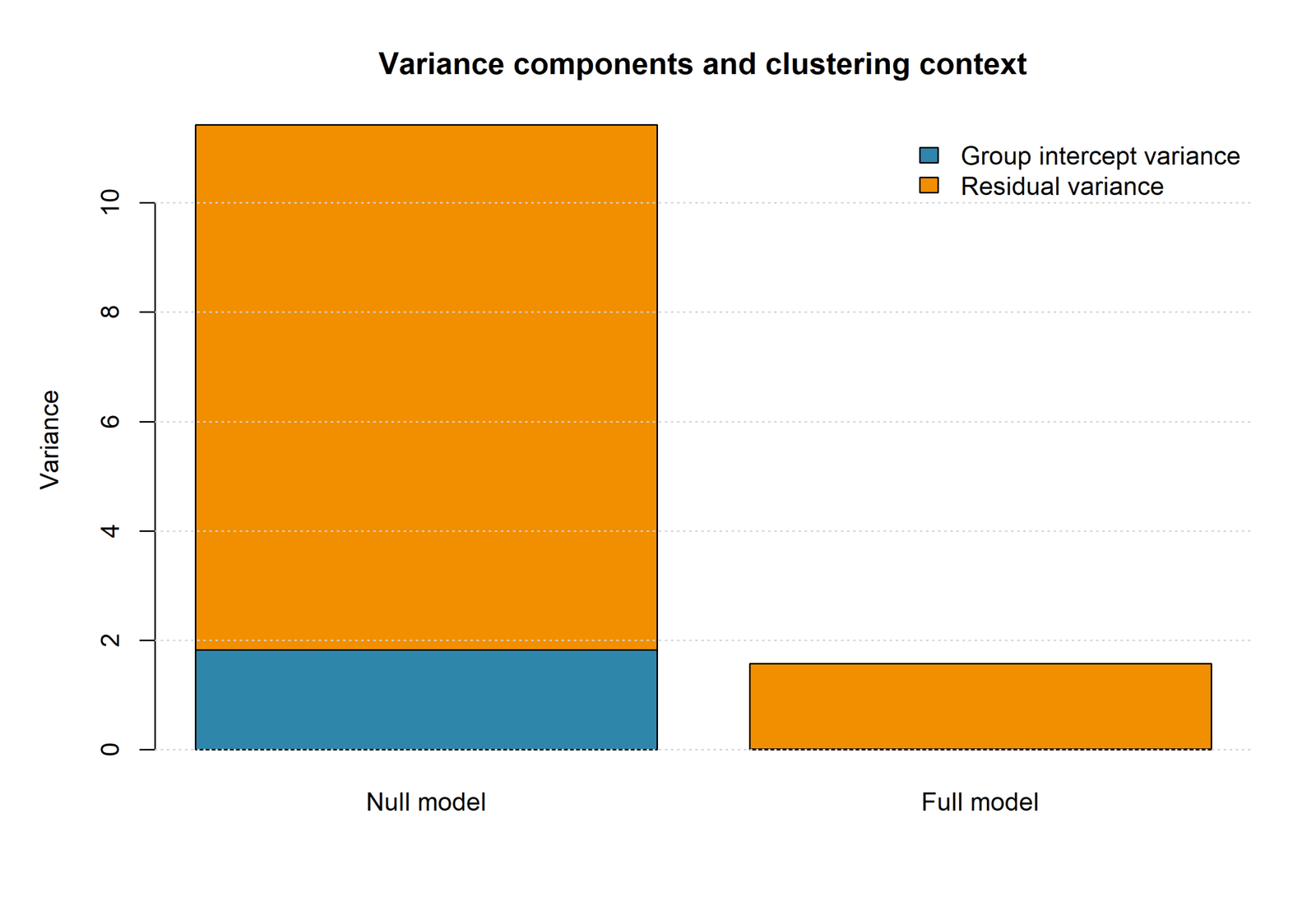
The R figures are paired so that each visual has its own aligned explanation. Together they emphasize the empty-to-full ICC reduction, the tiny conditional school effects, and the residual limits of the worked Multilevel Regression model.
R Chart 1: Empty and Full Variance Components
The empty model contains a visible between-school component, but the full model’s between-school segment becomes nearly invisible after the fixed predictors enter. R estimates empty-model school variance 1.822876 and residual variance 9.608405, giving ICC 0.159464. The full Multilevel Regression model estimates school variance 0.007738 and residual variance 1.565638, giving ICC 0.004918.
R Chart 2: Conditional School Random Intercepts
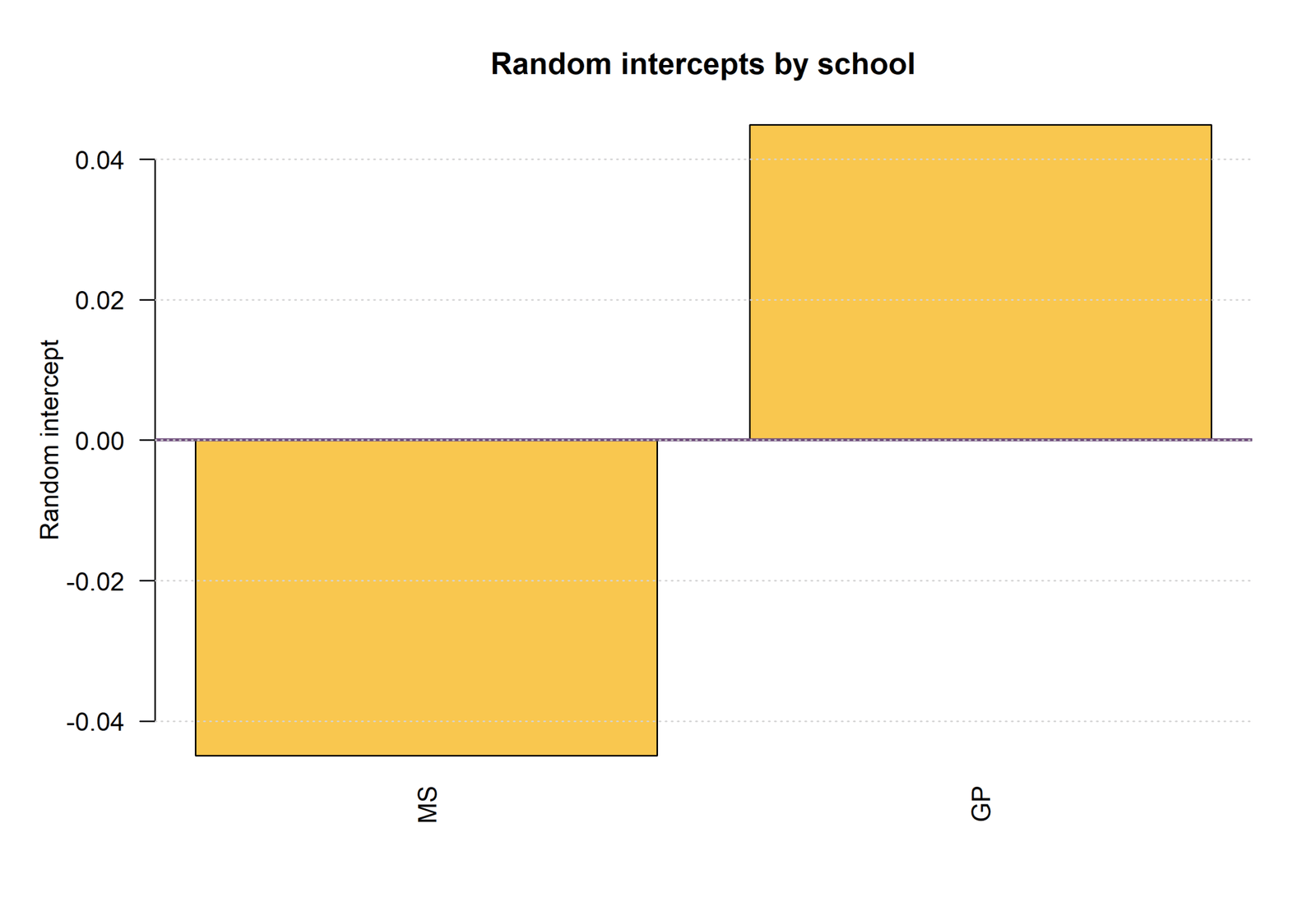
The bars point in opposite directions but are extremely small. GP is approximately +0.044945 and MS is -0.044945 after adjustment. The narrow vertical scale magnifies the appearance of separation. Relative to residual SD 1.251255 and the 0-to-19 outcome range, these Multilevel Regression school deviations are minor.
R Chart 3: Pearson Residual Distribution
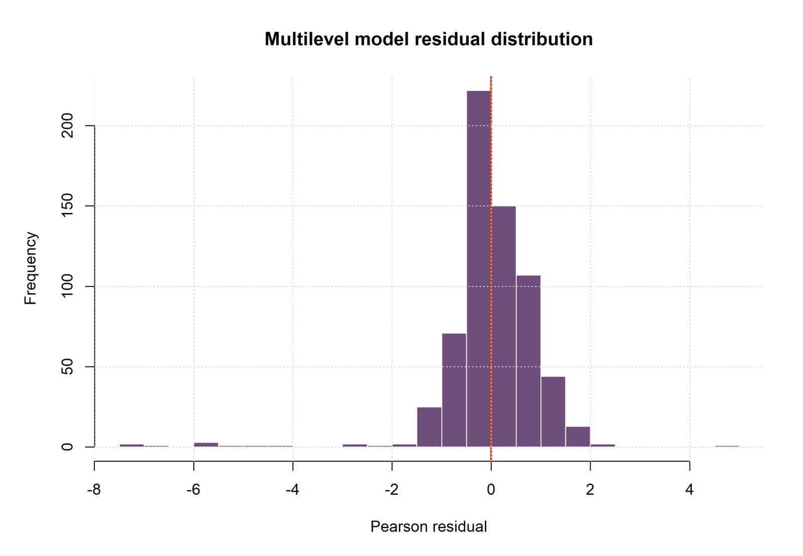
Most Pearson residuals cluster around zero, but the lower tail extends farther than the upper tail. The saved range is approximately -7.256 to 4.501. This asymmetry agrees with the raw-residual plots and shows that the Gaussian error approximation is imperfect for low final grades in the Multilevel Regression model.
R Chart 4: Final-Grade Distribution
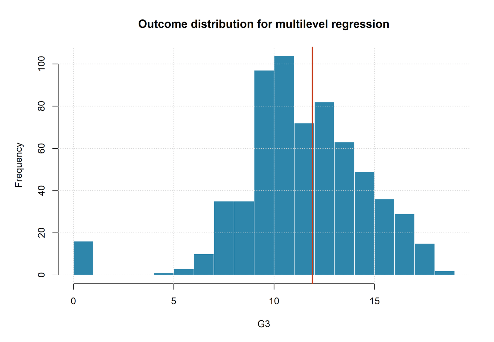
The R histogram reproduces the central grade concentration and the visible zero-grade group. The overall mean is 11.906009 and the observed range is 0 to 19. The agreement with the Python histogram confirms that both valid Multilevel Regression runs use the same 649 observations.
The R residual and fitted-value graphics should be read alongside
Residual Analysis
and the broader
Regression Diagnostics
workflow rather than treated as isolated pictures.
Multilevel Regression Coefficient and Parameter Interpretation
Interpreting Fixed Effects on the Correct Scale
Every coefficient in Multilevel Regression is conditional on the other entered predictors and the school random intercept. Python and R use raw outcome units. Python centers six numeric predictors, which changes the intercept but not the slope unit. SPSS standardizes ten numeric predictors, so its coefficient units differ.
Prior Grades: G1 and G2
Python estimates a G1 slope of 0.137545 and R estimates 0.134985. Holding the remaining variables and school intercept constant, a one-point higher first-period grade is associated with roughly 0.135 to 0.138 additional final-grade points. Both confidence intervals exclude zero.
The G2 slope dominates the Multilevel Regression equation. Python estimates 0.881011 and R estimates 0.880381. A one-point higher second-period grade is associated with about 0.88 additional final-grade points, conditional on the other variables. The narrow intervals show that this relationship is estimated much more precisely than most other fixed effects.
Failures
Python estimates -0.222574 and R estimates -0.222767 for failures. An additional prior failure is associated with about 0.223 lower final-grade points after adjustment. Both valid mixed outputs support the negative coefficient, and the broader SPSS OLS comparison also produces a negative standardized result.
Absences
The absences point estimate is positive in all three saved equations, but the inferential conclusion is not stable. Python gives 0.020646 with p < .001, R gives 0.019206 with p = .0825, and SPSS gives 0.088 per one standard deviation with p = .086. The Multilevel Regression evidence therefore does not support a robust absence effect.
A positive adjusted coefficient must not be converted into a causal claim that missing school improves grades. It can arise from conditioning on prior grades, nonlinearity, selection, measurement, omitted variables, or the distribution of high-absence cases. The disagreement in standard errors is an additional reason for caution.
Sex, Address, and Family Size
Python and R estimate a male coefficient near -0.20, but Python gives p = .0264 and R gives p = .0528. SPSS gives -0.168 with p = .118 in its broader standardized OLS model. The direction is consistent, but the threshold conclusion is not. A stable sex difference is not established.
The urban-address point estimates are 0.140931 in Python and 0.119674 in R. Python provides no standard error, so its result cannot be tested. R’s interval crosses zero. Family size estimates are small and uncertain in both valid Multilevel Regression runs.
Intercept and Random Intercepts
Python’s centered intercept of 11.867178 is the expected G3 for a female, rural, GT3 student at the sample means of the six centered numeric predictors, before the school deviation is added. R’s raw intercept is not directly comparable because its numeric predictors equal zero at the intercept reference point.
The school random effects are conditional offsets, not observed means and not causal impacts. R estimates +0.044945 for GP and -0.044945 for MS. Python estimates about +0.009654 and -0.009654. These values are tiny compared with the raw school mean difference because the fixed predictors absorb most of the observed composition gap.
Coefficient interpretation also depends on
Adjusted R-Squared
for fixed-only comparisons and
Null and Alternative Hypothesis
principles for deciding what each term-level test actually evaluates.
Predictions, Effects and Model Meaning
Conditional and Population-Level Predictions
A conditional prediction from Multilevel Regression combines the fixed part with the estimated school random intercept. A population-level or marginal prediction from the same linear predictor sets the random intercept to zero. For GP and MS, the difference is small because the fitted random effects are tiny.
Prediction for a student in a new school is different. The new school’s random effect is unknown, so the default prediction uses the fixed part unless information is available to estimate a new cluster deviation. Prediction uncertainty should then include both residual variation and the uncertainty associated with a new school’s random effect.
| Measure | Python ML | R REML | Interpretation |
|---|---|---|---|
| Fitted mean | 11.906009 | 11.906009 | Both reproduce the outcome mean |
| Fitted median | 11.691630 | 11.702114 | Nearly identical central prediction |
| Fitted minimum | 0.163407 | 0.163267 | Slightly above zero |
| Fitted maximum | 19.512157 | 19.533805 | Slightly above observed maximum 19 |
| RMSE | 1.242212 | 1.241070 | Nearly identical in-sample squared error |
| MAE | 0.778943 | 0.779027 | Nearly identical typical absolute error |
| Most negative residual | -9.049531 | -9.079313 | Large overprediction for low observed G3 |
| Most positive residual | 5.664255 | 5.631607 | Largest underprediction |
The Python and R Multilevel Regression predictions are almost identical despite the different estimators and centering conventions. That agreement reflects the near-zero adjusted school variance and the dominance of the fixed prior-grade slopes.
Worked Prediction Logic
For Python, the fixed intercept applies at the sample means of the centered numeric variables and the reference factor categories. A student’s centered G2 contribution is 0.881011 multiplied by the difference between that student’s G2 and the sample mean 11.5701. Similar calculations apply to the other centered numeric predictors.
The school contribution is only about +0.0097 for GP or -0.0097 for MS in Python. Therefore, two otherwise identical students assigned to the two saved school labels would receive conditional predictions differing by only about 0.0193 points. In R, the corresponding conditional difference is about 0.0899 points.
Prediction Limits
The observed-versus-fitted chart shows good central alignment but substantial error for some zero-grade cases. A Multilevel Regression prediction should not be interpreted as a guaranteed grade, a causal forecast, or a valid estimate for schools outside the data. The saved RMSE and MAE are in-sample quantities and are likely optimistic for new clusters.
Multilevel Regression Assumptions and Diagnostics
Grouping and Independence
Multilevel Regression assumes that school is the relevant grouping unit and that clusters are independent. The model does not represent classroom, teacher, neighborhood, or repeated-student dependence. If meaningful lower or higher clustering is omitted, the covariance structure may be incomplete.
Number of Level-2 Units
The most serious diagnostic limitation is not the 649-row sample size; it is the existence of only two schools. Random-effect variances, normality of school effects, cluster-level influence, and between-school generalization cannot be assessed reliably from two deviations. The adjusted ICC should therefore be presented as descriptive for GP and MS.
Linearity and Additivity
The fixed part assumes linear, additive relationships for G1, G2, study time, failures, absences, and age. The saved Multilevel Regression model contains no polynomial term, threshold, interaction, or school-specific slope. Residual plots should be checked for curvature, and plausible nonlinear grade or attendance effects should be evaluated in sensitivity analyses.
Random-Effect Distribution and Boundary Behavior
A conventional random-intercept model assumes school effects arise from a normal distribution with variance τ00. With only two schools, that distributional assumption cannot be diagnosed. The tiny Python variance and missing address standard error indicate boundary-adjacent estimation and an unstable covariance matrix.
A variance estimate of zero is permitted because variances cannot be negative. However, the usual likelihood-ratio reference distribution becomes nonstandard at the boundary. A naive chi-square test comparing the Python empty model with a no-random-effect model would not be justified.
Residual Normality and Constant Variance
The outcome is bounded and integer-valued, and both software residual summaries show a longer negative tail. Python raw residuals reach -9.049531, while R raw residuals reach -9.079313. These cases conflict with a simple symmetric normal-error description.
GP and MS also have different raw outcome standard deviations. The saved Multilevel Regression model uses one residual variance for both schools. A heterogeneous residual model, robust sensitivity analysis, or alternative outcome family may be considered, although only two schools still limit cluster-level inference.
Multicollinearity and Predictor Dependence
G1 and G2 are strongly related prior-grade measures. Their joint inclusion is substantively defensible, but it changes the meaning and uncertainty of each coefficient. Centering does not reduce ordinary collinearity created by correlated predictors. Variance inflation, condition indices, and coefficient stability should be reviewed in the fixed design.
Influential Observations and Clusters
Large negative residuals identify students whose final grades are far below the model’s fitted values. They should be reviewed for data quality, unusual circumstances, and influence. A residual outlier is not automatically influential. Case-deletion diagnostics and fixed-effect changes are needed.
Cluster influence cannot be meaningfully distributed across many schools because there are only two. Removing either GP or MS eliminates the level-2 comparison. That fact reinforces the descriptive boundary of this Multilevel Regression application.
Evidence that supports the model
- Complete selected variables for all 649 students
- Consistent G1, G2, and failures slopes across Python and R
- Nearly identical fitted-error summaries
- Clear distinction between empty and adjusted variance
Evidence that limits the model
- Only two schools
- Python singular covariance and missing address SE
- Long negative residual tail
- Common residual variance despite different raw school spread
- No valid SPSS mixed output
A complete diagnostic extension can combine
Regression Assumptions,
Q-Q Plot Normality Check,
Breusch-Pagan Test,
Variance Inflation Factor,
Tolerance Statistic,
Cook’s Distance,
Influence Diagnostics, and
Durbin-Watson Test.
Some of these procedures are fixed-model diagnostics, so they supplement rather than replace cluster-level checks.
Multilevel Regression in Python, R, SPSS and Excel
Software Roles in the Worked Analysis
Python Multilevel Regression
- Grand-mean centers six numeric predictors
- Fits OLS, empty, and full
MixedLMmodels - Uses maximum likelihood
- Exports coefficients, variance components, predictions, residuals, and charts
- Requires a covariance audit because one fixed-effect SE is missing
R Multilevel Regression
- Uses raw numeric predictors
- Fits
nlme::lmerandom-intercept models - Uses REML for the saved final fit
- Provides finite fixed-effect uncertainty, ICC, predictions, and random effects
- Supplies the most internally complete mixed output
SPSS Audit
- Creates z scores and binary indicators
- Successfully fits a broader standardized OLS model
- Fails at both
MIXEDcommands becauseFITis invalid in/PRINT - Creates no mixed predictions or residuals
- Must be corrected and rerun before SPSS multilevel claims are made
Excel Companion
- Demonstrates grand-mean centering
- Shows the ICC formula from variance components
- Provides fixed-effect interpretation templates
- Supports arithmetic tracing and reporting
- Does not estimate a random-effects covariance matrix by ordinary worksheet formulas
Cross-Software Reconciliation
The one planned cross-check for Multilevel Regression establishes that Python and R use the same 649 records and produce nearly identical fixed slopes, fitted values, RMSE, and MAE. Differences in intercepts follow from centering. Differences in variance estimates and standard errors follow from ML versus REML, optimizer and covariance implementation, and boundary behavior.
SPSS is not a third mixed-model replication. Its saved output is valuable because it documents exactly where the mixed workflow failed. The valid OLS table can be used as a fixed-only sensitivity comparison, provided its broader predictor set and standardized numeric scales are stated.
Which Output Should Lead the Report?
R is the strongest primary source for term-level Multilevel Regression uncertainty because every fixed coefficient has a finite standard error and interval. Python remains useful for the centered intercept, predictions, charts, and the demonstration of boundary instability. The software should be synthesized rather than forced into artificial numerical agreement.
For alternative covariance and design strategies, compare the present random-intercept analysis with
Fixed Effects Regression and
Generalized Least Squares Regression.
The choice depends on the estimand, cluster structure, and assumptions about unobserved group differences.
Code: Expand Only the Software You Need
The code blocks below preserve the important distinctions in the saved Multilevel Regression workflow. They are examples of the core specification rather than substitutes for the full downloadable reports and scripts.
Python: centered maximum-likelihood random-intercept model
numeric = ["G1", "G2", "studytime", "failures", "absences", "age"]

for column in numeric:
    data[f"c_{column}"] = data[column] - data[column].mean()

formula = (
    "G3 ~ c_G1 + c_G2 + c_studytime + c_failures + "
    "c_absences + c_age + C(sex) + C(address) + C(famsize)"
)

model = smf.mixedlm(
    formula,
    data=data,
    groups=data["school"],
    re_formula="1"
)
fit = model.fit(reml=False, method="lbfgs", maxiter=1000, disp=False)

tau00 = float(fit.cov_re.iloc[0, 0])
sigma2 = float(fit.scale)
icc = tau00 / (tau00 + sigma2)
The Python Multilevel Regression code centers six numeric predictors, fits one random school intercept by ML, and derives the ICC from the fitted variance components. After fitting, every standard error and covariance warning must be checked before significance labels are assigned.
R: raw-unit REML random-intercept model
library(nlme)

fit_r <- lme(
  fixed = G3 ~ G1 + G2 + studytime + failures + absences +
    age + sex + address + famsize,
  random = ~ 1 | school,
  data = analysis_data,
  method = "REML",
  na.action = na.omit
)

vc <- VarCorr(fit_r)
tau00 <- as.numeric(vc[1, "Variance"])
sigma2 <- as.numeric(vc[2, "Variance"])
icc <- tau00 / (tau00 + sigma2)

fixed_table <- summary(fit_r)$tTable
conditional_predictions <- fitted(fit_r, level = 1)
raw_residuals <- residuals(fit_r, type = "response")
The R Multilevel Regression code retains original numeric units and uses REML. Confidence intervals should be calculated from the reported coefficient estimates and degrees of freedom rather than copied from an unrelated software table.
SPSS: corrected MIXED print specification
* The saved command failed because FIT was included in /PRINT.
MIXED G3 WITH ZG1 ZG2 Zstudytime Zfailures Zabsences Zage
  ZMedu ZFedu Ztraveltime Zhealth sex_M address_U higher_yes
  internet_yes schoolsup_yes famsup_yes activities_yes
  /FIXED=INTERCEPT ZG1 ZG2 Zstudytime Zfailures Zabsences Zage
  ZMedu ZFedu Ztraveltime Zhealth sex_M address_U higher_yes
  internet_yes schoolsup_yes famsup_yes activities_yes | SSTYPE(3)
  /METHOD=ML
  /PRINT=SOLUTION TESTCOV
  /RANDOM=INTERCEPT | SUBJECT(school) COVTYPE(VC)
  /SAVE=FIXPRED PRED RESID.
This correction removes the invalid FIT keyword. A valid SPSS Multilevel Regression report still requires rerunning the command and verifying that the fixed solution, covariance parameters, predictions, residuals, SPV, and PDF are actually created.
Excel: centering and ICC arithmetic
Centered predictor:
=RawValue - AVERAGE(AllRawValues)

ICC from variance components:
=BetweenSchoolVariance /
 (BetweenSchoolVariance + WithinSchoolVariance)

Conditional prediction:
=FixedPart + SchoolRandomIntercept
Excel can trace the arithmetic used after a Multilevel Regression model has supplied coefficients and variance components. It should not be presented as independently estimating the random-effects likelihood or covariance matrix unless a specialized implementation has been built and validated.
Advanced Multilevel Regression Topics
The following panels extend the worked Multilevel Regression analysis beyond the basic coefficient table. They focus on design, estimation, centering, variance interpretation, prediction, diagnostics, and software reconciliation.
1. Defining Level 1 and Level 2
In this worked Multilevel Regression analysis, a student is the level-1 observational unit and school is the level-2 cluster. Level 1 contains the outcome and all measured predictors used in the valid Python and R mixed equations. Level 2 contains only the grouping label because no school-level covariate is available.
The distinction is more than terminology. Student-level slopes use 649 rows, whereas the school-intercept variance is informed by two schools. A large level-1 sample can estimate stable individual slopes while leaving the random component poorly identified. Multilevel Regression reporting should therefore state both counts rather than presenting 649 as the effective sample size for every parameter.
2. Random Intercepts and Shared Covariance
A random intercept gives all students in school j the same fitted deviation u0j. In Multilevel Regression, two students from the same school share that deviation, creating model-implied covariance equal to the between-school variance τ00. Students from different schools do not share it.
The saved Python and R estimates show that this shared adjusted component is tiny. The random intercept still performs a conceptual role by separating cluster dependence from individual residual error. It does not imply that every student in GP receives the same fitted grade; their fixed predictor values and residuals remain different.
3. Empty-Model ICC Versus Conditional ICC
The empty Multilevel Regression model asks how final-grade variance is divided before predictors enter. R estimates ICC 0.159464, so about 15.95% of unconditional modeled variance is associated with the school intercept. The full model asks the same question after adjustment and gives ICC 0.004918.
The reduction is a composition result. Prior grades and other student characteristics account for most of the raw school separation. It is incorrect to report only the adjusted ICC and conclude that the original data were never clustered. The two ICCs answer different questions and should be presented together.
4. Why Two Clusters Are a Serious Limitation
The random part of Multilevel Regression depends primarily on the number of clusters, not just the number of observations. Two schools provide only two empirical intercept deviations. They cannot reveal the shape, skew, tails, or normality of a wider school-effect distribution.
Standard errors for fixed effects may also be fragile when the random variance is near zero and the cluster count is minimal. The correct response is not to hide the limitation or to treat 649 as 649 independent schools. The result should be described as a two-school conditional decomposition, with broader school-population claims deferred until many more level-2 units are observed.
5. Grand-Mean Centering
Python grand-mean centers six numeric predictors before fitting Multilevel Regression. Centering subtracts the overall sample mean but does not divide by the standard deviation. A one-unit change in centered G2 remains a one-grade-point change.
The main benefit is intercept interpretation. Python’s intercept refers to a female, rural, GT3 student at average values of the six numeric predictors, before the school effect is added. Centering does not remove confounding, does not create within-school effects automatically, and does not solve the two-cluster problem.
6. Cluster-Mean Centering and Contextual Effects
Grand-mean centering is not the same as cluster-mean centering. A cluster-mean-centered predictor subtracts the school-specific mean and isolates within-school deviation. A separate school mean can then represent between-school composition. That decomposition is often central to Multilevel Regression.
The saved analysis does not perform this decomposition. Its G1 and G2 coefficients combine within-school and between-school information under the random-intercept assumptions. With only two schools, estimating contextual school-mean effects would also be extremely unstable, but the distinction remains important for interpretation.
7. Fixed Effects Versus Random Effects
Fixed effects in Multilevel Regression are population-average coefficients shared across the modeled schools. Random effects are fitted cluster deviations around the fixed intercept. The two parts answer different questions and use different sources of information.
A fixed school dummy would estimate a separate contrast for GP versus MS without assuming that the two schools are sampled from a normal distribution. A random school intercept instead estimates a variance component and shrinks the school deviations toward zero. With only two named schools, a fixed-school sensitivity model can be informative, but it does not produce a general school variance or ICC.
8. Random Slopes
A random-slope Multilevel Regression model would allow a predictor such as G2 to have different slopes across schools. Its equation would include an additional school-specific term u1jG2. The saved models contain no such term.
Only two schools make random-slope variance essentially unidentifiable as a population parameter. A descriptive interaction between school and G2 could be examined, but it would represent the difference between GP and MS rather than a stable distribution of slopes across schools.
9. Cross-Level Interactions
A cross-level interaction asks whether a level-1 slope changes as a function of a level-2 characteristic. For example, a school-resource measure might modify the relationship between study time and final grade. This is a common extension of Multilevel Regression.
No measured school-level predictor is available in the worked file, so no cross-level interaction can be estimated. Using the school label itself as an interaction creates a two-group slope comparison, not a general contextual moderation effect. Clear variable-level identification prevents overstatement.
10. ML Versus REML
Python uses maximum likelihood and R uses restricted maximum likelihood for the saved Multilevel Regression fits. ML estimates fixed and random parameters within one likelihood and is commonly used for comparing models with different fixed-effect structures. REML adjusts variance estimation for the fixed effects and is often preferred for a final model with a fixed specification.
The saved AIC and log-likelihood values should not be directly ranked across Python and R because the estimation criteria differ. Cross-software agreement should focus on the slopes, predictions, residuals, and variance conclusion rather than forcing likelihood values into one league table.
11. Boundary and Singular Fits
Variance parameters cannot be negative, so zero is a boundary of the parameter space. When a Multilevel Regression estimate approaches zero, the Hessian can become nearly singular and standard asymptotic approximations may fail.
Python’s tiny school variance, missing address standard error, and software-sensitive standard errors are practical signs of this problem. A singular fit is not automatically proof that the model is useless. It is a warning that the random structure is weakly supported and that term-level Wald tests require sensitivity checks or alternative uncertainty methods.
12. Likelihood-Ratio Testing at the Boundary
A conventional likelihood-ratio test assumes that the null parameter lies in the interior of the parameter space. Testing whether a random-effect variance equals zero violates that assumption because zero is the boundary. The reference distribution is therefore not the usual simple chi-square distribution.
For the Python Multilevel Regression empty model, the school variance collapses to zero. A naive regular chi-square comparison should not be used to declare the random intercept significant or nonsignificant. Parametric bootstrap methods or appropriate mixture references are preferable when the design contains enough clusters to justify the exercise.
13. Degrees of Freedom and Small-Sample Inference
Different Multilevel Regression software uses different approximations for denominator degrees of freedom and fixed-effect uncertainty. R’s nlme output uses a t-based framework, while Python’s saved MixedLM table uses large-sample z approximations.
With only two clusters, neither framework can create information that the design lacks. Methods such as Satterthwaite or Kenward-Roger adjustments are valuable in many multilevel studies, but they still require a reasonable cluster sample. The software label should never substitute for a design-based assessment of inferential support.
14. Interpreting the School Random Effects
R estimates conditional school deviations of +0.044945 for GP and -0.044945 for MS. Python gives approximately +0.009654 and -0.009654. In Multilevel Regression, these empirical predictions are shrunken estimates, not raw school means.
The values apply after the fixed predictors enter. They are small because the prior grades and other characteristics explain most of the original mean difference. They should not be ranked as school quality scores, used for causal accountability, or generalized beyond the two observed institutions.
15. Conditional and Marginal Predictions
A conditional Multilevel Regression prediction includes the estimated random intercept for a known school. A marginal or population-level prediction sets that school deviation to zero. The distinction matters most when the random variance is large.
In this analysis, conditional and marginal predictions are very close because the adjusted school effects are tiny. For a new school, the random effect is unknown. The fixed part gives the default prediction, and uncertainty should include possible between-school variation rather than borrowing GP or MS’s fitted deviation.
16. Prediction for New Clusters
Predicting a new student in GP or MS uses a known fitted school effect. Predicting a student in an unseen school is a new-cluster problem. A robust Multilevel Regression evaluation should therefore leave out entire clusters, not randomly split students while retaining both schools in training and testing.
Whole-cluster validation is impossible with only two schools because leaving one out leaves no distribution of training clusters. The reported RMSE and MAE are in-sample and should not be advertised as evidence of generalization to other schools.
17. Heterogeneous Residual Variance
The saved Multilevel Regression model assumes one within-school residual variance. Yet GP’s raw final-grade SD is 2.625636 and MS’s is 3.833991. Some of that difference may be explained by predictors, but the assumption deserves a residual-level check.
R can model different residual spreads by school through an appropriate variance function. Such a sensitivity analysis may improve fit, but two groups still provide limited evidence for a general heteroscedastic pattern. The goal is to test whether the common-variance assumption distorts fixed-effect uncertainty, not merely to add complexity.
18. Bounded and Discrete Outcomes
G3 is observed as an integer from 0 to 19. The Gaussian Multilevel Regression model treats it as approximately continuous and can produce fitted values slightly outside the observed range. Python and R fitted maxima exceed 19 by about half a point.
The central fit is strong, but the zero-grade cases create a long negative residual tail. Sensitivity options include robust standard errors, ordinal or bounded-outcome models, or explicitly modeling the low-grade process. The appropriate alternative depends on the substantive meaning of the scale and the prediction target.
19. Nonlinearity and Interactions
The saved Multilevel Regression equation is linear and additive. It assumes that each extra G2 point has the same expected association with G3 across the observed range and that failures or absences do not change that slope.
Residual curvature, theory, or out-of-range predictions can motivate polynomial terms, splines, or interactions. Any extension should be prespecified or validated and should not be justified solely by a small in-sample improvement. The two-school structure also prevents reliable random-slope complexity.
20. Multicollinearity and Prior Grades
G1 and G2 are related measures of previous performance. In Multilevel Regression, each coefficient represents its association with final grade after holding the other prior grade constant. That conditional meaning is narrower than a simple correlation.
Strong predictor correlation can inflate standard errors and make coefficients sensitive to specification. Centering does not remove this form of collinearity. Variance inflation factors, condition indices, and models that include each prior grade separately can help explain the stability of the final conclusions.
21. Missing Data
The selected Python and R variables are complete, so the saved Multilevel Regression analysis uses all 649 rows. This avoids differences caused by software-specific listwise deletion in the current model.
In a broader study, missingness can occur at both student and school levels. Complete-case analysis may alter cluster composition and bias effects if missingness is informative. Multilevel multiple imputation should preserve the hierarchy and include cluster indicators or random structures appropriate to the imputation model.
22. Influential Students and Influential Schools
Large residuals identify poorly predicted students, but influence depends on how much deleting a case changes the fitted Multilevel Regression coefficients or variance components. The zero-grade cases deserve review because their negative residuals approach -9.
Cluster influence is even more consequential. With only GP and MS, deleting either school destroys the intended random-effect analysis. This means the between-school conclusion is structurally dependent on both clusters and cannot be tested through ordinary leave-one-cluster-out diagnostics.
23. Marginal and Conditional R-Squared
Marginal R² for Multilevel Regression summarizes variance explained by the fixed effects, whereas conditional R² includes both fixed and random effects. When the adjusted school variance is near zero, the two quantities should be almost identical.
The saved package reports an OLS comparison R² around 0.852 and an SPSS fixed-only R² of 0.854 under a broader predictor set. Those values are not automatically the formal marginal R² of the mixed models. A report should name the exact calculation rather than relabeling ordinary R².
24. Reconciling Python, R, and SPSS
A sound Multilevel Regression audit compares like with like. Python and R use the same substantive nine predictors but differ in centering and estimator. SPSS uses a broader standardized fixed equation and fails before producing mixed output.
The correct synthesis is not to average coefficients or choose the smallest p-value. It is to identify the replicated slopes, explain scale differences, report estimator-specific variance components, and state that SPSS contributes only the valid OLS comparison and the execution warning.
25. APA Reporting with a Two-Cluster Caveat
An APA-style Multilevel Regression paragraph should name the outcome, grouping variable, cluster count, estimator, fixed predictors, variance components, ICC, key coefficients, and diagnostic limitations. It should distinguish the empty-model ICC from the adjusted ICC.
The two-school limitation belongs in the primary results, not only in a footnote. Terms whose software conclusions differ should be described as uncertain. The missing Python address standard error and failed SPSS mixed command should be reported transparently rather than omitted.
26. Decision Checklist for Future Analyses
Before fitting Multilevel Regression, confirm the hierarchy, count level-2 units, define fixed and random effects, choose centering, inspect outcome support, and decide whether ML or REML matches the comparison goal. After fitting, review convergence, singularity, variance components, residuals, influential cases, and prediction target.
For this dataset, the checklist leads to a narrow decision: retain the model as a descriptive two-school adjustment, report the stable G1, G2, and failures effects, treat the adjusted ICC cautiously, avoid SPSS mixed claims until rerun, and do not generalize the school variance beyond GP and MS.
Further extensions include
Bayesian Regression
for full posterior uncertainty,
Statistical Power
for planning cluster counts, and
Type I and Type II Error
for understanding the consequences of unstable small-cluster inference.
APA-Style Reporting
Primary Multilevel Regression Report
A random-intercept Multilevel Regression model was fitted to final grades for 649 students nested in two schools. In the R REML analysis, the empty model estimated between-school variance of 1.822876 and within-school variance of 9.608405, yielding ICC = .159464. After G1, G2, study time, failures, absences, age, sex, address, and family size were entered, between-school variance decreased to 0.007738 and residual variance to 1.565638, yielding conditional ICC = .004918.
Higher G1 was associated with higher final grade, B = 0.134985, SE = 0.036691, p < .001, 95% CI [0.062935, 0.207035]. Higher G2 was also positively associated with final grade, B = 0.880381, SE = 0.034162, p < .001, 95% CI [0.813298, 0.947464]. Prior failures showed a negative association, B = -0.222767, SE = 0.094977, p = .0193, 95% CI [-0.409272, -0.036262]. Other fixed effects were not clearly supported at .05.
Software Sensitivity Statement
The centered Python maximum-likelihood Multilevel Regression model produced similar point estimates and an adjusted ICC of .000568, but its covariance calculation was partly singular and no standard error was available for address. Python identified sex and absences as significant, whereas R did not; those effects were therefore treated as software-sensitive rather than replicated.
SPSS Audit Statement
The saved SPSS output did not contain a valid Multilevel Regression fit because the MIXED commands stopped at an invalid FIT option in the /PRINT subcommand. The successful SPSS result was a broader standardized OLS comparison, R² = .854, adjusted R² = .850, F(17, 631) = 217.194, p < .001. No SPSS mixed-model variance component or ICC was reported.
Publication Checklist
Before Publication
- State that students are nested in two schools.
- Name
G3as the level-1 outcome and school as the level-2 grouping variable. - Separate the empty-model ICC from the adjusted ICC.
- Identify Python as centered ML and R as raw-unit REML.
- Do not compare SPSS standardized coefficients directly with raw-unit slopes.
- Report the missing Python address standard error.
- Describe sex and absences as software-sensitive.
- State that SPSS MIXED failed and was not interpreted.
Before Reusing the Model
- Collect many more schools.
- Predefine fixed and random effects.
- Check centering and reference categories.
- Inspect residual tails and zero-grade cases.
- Evaluate nonlinear terms and interactions when justified.
- Check singularity and covariance stability.
- Validate by whole-cluster prediction.
- Use a consistent estimator for formal model comparison.
A complete Multilevel Regression report should let a reader reconstruct the hierarchy, scale, estimator, variance decomposition, coefficient interpretation, diagnostic limits, and software boundaries without guessing.
Downloads and Chart Resources
Same-Topic Reports and Worked Workbook
These resources support the worked Multilevel Regression article. The Python and R PDFs contain the valid mixed analyses. The SPSS PDF is retained because it documents the valid OLS comparison and the exact failure of the mixed commands. The workbook traces calculations but is not an independent random-effects estimator.
Frequently Asked Questions
These questions summarize the interpretation, software, and diagnostic decisions that matter most in the worked Multilevel Regression analysis.
What makes this analysis multilevel?
Students are level-1 observations nested within the level-2 school variable. The Multilevel Regression model gives students from the same school a shared random intercept, so their conditional outcomes are not treated as completely independent.
How many schools are included?
There are two schools: GP with 423 students and MS with 226. The 649 rows provide information about student-level slopes, but only two cluster deviations inform the Multilevel Regression school variance.
What is the empty-model ICC?
The R empty-model ICC is 0.159464, based on between-school variance 1.822876 and residual variance 9.608405. It describes unconditional school clustering before the fixed predictors enter the Multilevel Regression equation.
What is the adjusted ICC?
R estimates adjusted ICC 0.004918, and Python estimates 0.000568. Both Multilevel Regression fits indicate that almost all remaining modeled variance is within schools after student predictors are included.
Why do the raw school means differ more than the random intercepts?
Raw means do not adjust for prior grades, failures, attendance, or other composition. The Multilevel Regression random intercept is the residual school baseline after those predictors are held constant, so it is much smaller.
What is grand-mean centering?
Grand-mean centering subtracts the full-sample mean from each numeric predictor. Python uses it for six variables. In the same additive Multilevel Regression model, centering changes the intercept but preserves the original slope units.
Does centering make a coefficient a within-school effect?
No. Grand-mean centering alone does not separate within-school and between-school information. That requires cluster-mean centering plus the cluster mean or another explicit decomposition in the Multilevel Regression model.
Which fixed effects are most reliable?
The replicated Multilevel Regression evidence supports positive G1 and G2 slopes and a negative failures slope. These directions and inferential conclusions agree across the valid Python and R mixed outputs.
Why are sex and absences treated cautiously?
Python labels both terms significant, while R does not. Their point estimates are similar but their standard errors differ. Because Python also has a singular covariance problem, the Multilevel Regression evidence for sex and absences is software-sensitive.
Can the Python address coefficient be interpreted?
The point estimate can be stated descriptively, but the missing standard error means no valid Python p-value or confidence interval is available. The Multilevel Regression address effect should therefore rely on the finite R estimate and its uncertainty.
Did SPSS fit a multilevel model?
No. Both saved SPSS MIXED commands stop because FIT is invalid in the /PRINT subcommand. The SPSS file provides a valid standardized OLS comparison but no valid Multilevel Regression variance component or ICC.
Can the SPSS G2 coefficient be compared directly with R?
No. SPSS enters standardized G2, while R uses raw grade points. The coefficients represent different predictor units. A proper Multilevel Regression comparison must first put estimates on the same scale.
Are the Python and R AIC values directly comparable?
Not as saved. Python uses ML and R uses REML, and their parameterization and centering differ. The Multilevel Regression audit should compare like-for-like fits under the same likelihood before ranking AIC values.
Are the residuals normally distributed?
They are centered near zero but have a longer negative tail, with raw residuals around -9 for some students. The Gaussian Multilevel Regression approximation is useful but imperfect, especially for zero-grade cases.
Can this model predict a new school?
It can produce a fixed-part prediction for a student in a new school, but the new random intercept is unknown. Reliable new-school validation of Multilevel Regression requires many clusters and whole-cluster testing.
What would improve this analysis most?
The most important improvement is collecting many more schools. That would support stable variance estimation, random-slope evaluation, cluster influence checks, whole-school validation, and a more defensible population interpretation of Multilevel Regression.
Multilevel Regression Conclusion
Final Interpretation
The worked Multilevel Regression analysis separates a visible raw school difference from the much smaller conditional school variance that remains after adjustment. GP and MS differ by about 1.926 points in unadjusted mean final grade, and the R empty model estimates ICC 0.159464. After prior grades and other student predictors enter, the R ICC falls to 0.004918 and the Python ICC to 0.000568.
The strongest fixed-effect evidence is consistent across the valid mixed runs. Higher G1 and G2 are associated with higher final grades, while prior failures are associated with lower final grades. Sex and absences have similar point estimates across software but different uncertainty, so they should not be presented as replicated findings. The missing Python address standard error confirms that the Python covariance matrix is not fully regular.
The SPSS output adds an important audit result rather than a third Multilevel Regression replication. Its standardized OLS model runs, but both mixed commands stop before estimation because of an invalid print option. No SPSS mixed coefficient, random effect, variance component, prediction, residual, or ICC should be reported from that file.
The final conclusion is deliberately narrow. In these 649 student records, measured student characteristics explain almost all adjusted intercept separation between GP and MS, and the conditional predictions are driven overwhelmingly by the fixed prior-grade slopes. Because only two schools are observed, the random-effect estimates remain descriptive. A general statement about school-to-school variation requires many more level-2 units, stable covariance estimation, and whole-cluster validation.
For the next stage of analysis, use the linked guides on
Random Effects Regression
and
Influence Diagnostics
to compare alternative group-effect assumptions and identify observations that may disproportionately affect the fitted model.

