
Regression Assumptions: Tests, Diagnostics, Python, R, SPSS and Excel Guide
Regression Assumptions determine whether a fitted linear model gives a defensible description of the conditional mean and trustworthy uncertainty estimates. This worked audit evaluates functional form, residual distribution, variance stability, independence, multicollinearity, leverage, and influence for a 649-case model of G3.
Regression Assumptions Model Overview
Regression Assumptions are the conditions under which an ordinary least squares model can be interpreted as an adequate linear description of the outcome and its conventional standard errors, confidence intervals, t tests, and F tests can be trusted. They are not one universal pass-or-fail checklist. Each assumption asks a different question, uses different evidence, and may require a different remedy. Regression Assumptions evidence should always be linked to the exact fitted specification.
What Regression Assumptions Are
The fitted equation predicts G3 from G1, G2, studytime, failures, absences, and age. The model can have a high R² while still violating functional-form, variance, or residual-distribution conditions. Regression Assumptions therefore evaluate the structure left behind after the mean equation is fitted rather than judging the model only from R² or the overall F statistic.
The most important conditions are an adequately specified conditional mean, independent errors, stable residual variance, acceptable residual behavior for the intended inference, manageable multicollinearity, and absence of cases that determine results disproportionately.
Why Regression Assumptions Must Be Checked Separately
A normal residual histogram does not prove constant variance. A Durbin-Watson value near 2 does not prove linearity. A VIF below 5 does not prove that no observation is influential. Each diagnostic targets a distinct feature of the model.
The current audit is deliberately mixed. Independence and collinearity are reasonably supported. Functional form, homoscedasticity, and residual normality are challenged. Influence diagnostics identify a limited but important group of cases. The correct conclusion is therefore not “all assumptions pass” or “the model is invalid,” but a condition-by-condition interpretation.
The Worked Regression Model
The model uses 649 complete observations and six predictors. R² is 0.8506322461601578, adjusted R² is 0.8492362858438975, RMSE is 1.2544090063688753, and the overall model is significant, F = 609.3527418021525, p < .001.
Linearity and Functional Form
Linearity means that the specified additive terms adequately represent the conditional mean. It does not mean that every raw scatterplot must be a perfect straight line. The question is whether systematic curvature or omitted combinations remain after all predictors are considered.
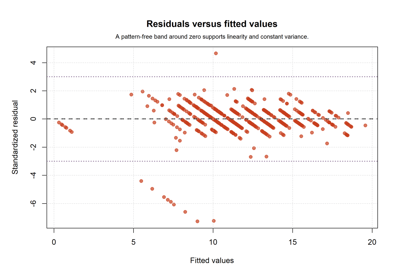
The Ramsey RESET Test gives F = 10.77405708716365, p = 0.0010852315202711362. This challenges the current functional form and suggests that nonlinear terms, interactions, transformations, or omitted structure may remain.
Homoscedasticity
Homoscedasticity means that conditional residual variance is approximately constant across fitted values and predictor profiles. It is not required for OLS coefficient estimates to be computed, but it is important for conventional model-based standard errors.
The Breusch-Pagan Test gives LM = 33.0541920131443, p = 1.0237048600284003 × 10⁻⁵. The White Test gives LM = 75.54743490382064, p = 1.7528560789176337 × 10⁻⁶. Both reject constant variance.
Residual Normality
Residual normality is mainly an inferential condition for exact small-sample tests and intervals. It is not required for the OLS line to minimize squared error. In large samples, coefficient estimates may remain useful despite non-normal residuals, but extreme tails can affect uncertainty and influence.
The Shapiro-Wilk Test gives W = 0.754697364131062, p = 6.244475451873078 × 10⁻³⁰. The Jarque-Bera Test gives JB = 10152.729452009393, p approximately 0. The histogram and Q-Q plot show that this result is driven largely by strong tail departures and unusual low-outcome cases.
Independence of Errors
Independence means that one observation’s error is not systematically connected to another’s. This is primarily a study-design issue. The residual sequence and Durbin-Watson statistic can detect some order-related structure when row order has a meaningful sequence.
Durbin-Watson is 1.8609563415688704, reasonably close to 2. The evidence does not indicate strong first-order autocorrelation, although this does not prove independence under every possible clustering mechanism.
Multicollinearity
Multicollinearity concerns overlap among predictors. High overlap can inflate coefficient standard errors and make individual slopes unstable even when overall prediction remains strong.
The maximum VIF is 4.154856661640564 for G1, followed by 4.091388386290769 for G2. Both are below the selected guideline of 5. The scaled-predictor condition number is 4.250229914028819, also modest. The audit therefore treats collinearity as acceptable, while recognizing that G1 and G2 share substantial information.
Outliers, Leverage and Influence
An outlier has an unusual outcome error. A high-leverage case has an unusual predictor profile. An influential case changes fitted results materially when deleted. These concepts overlap but are not interchangeable.
The audit uses |externally studentized residual| > 3, leverage > 0.02157164869029276, Cook’s distance > 0.0061633281972265025, and |DFFITS| > 0.2077096468163805. Ten cases exceed the residual rule, 45 exceed the leverage rule, 26 exceed the Cook’s distance rule, 26 exceed the DFFITS rule, and 58 trigger at least one flag.
What Violations Mean
A violation does not automatically require abandoning the model. Functional-form evidence may motivate nonlinear terms or interactions. Heteroskedasticity may motivate robust standard errors, transformation, weighted least squares, or a modeled variance. Non-normal tails may motivate robust inference or sensitivity analysis. Influential observations require case review and refitting comparisons.
Advantages of a Full Assumption Audit
- Separates prediction quality from inferential validity.
- Identifies the specific model feature needing attention.
- Prevents a single normality test from dominating the conclusion.
- Links graphical evidence with formal statistics.
- Shows whether results depend on a small number of observations.
- Supports transparent remedial decisions.
Limitations
- Formal tests can detect trivial departures in large samples.
- Thresholds such as VIF 5 or Cook’s 4/n are guidelines, not laws.
- Plots require judgment.
- Passing one diagnostic does not prove an assumption universally.
- Remedies can change the estimand or interpretation.
- Data quality and study design cannot be repaired by diagnostics alone.
Quick Answer
Conditions challenged
- Functional form
- Constant variance
- Residual normality
- Influence sensitivity
Conditions reasonably supported
- No strong first-order residual autocorrelation
- VIF values below 5
- Scaled condition number well below 30
- Strong overall model fit
Table of Contents
- Quick Answer
- Why This Analysis Needs Regression Assumptions
- How Regression Assumptions Are Evaluated
- Variables and Model Specification
- Formal Regression Assumptions Results
- Ten Python Chart Stories
- Four R Charts and Explanations
- Condition-by-Condition Interpretation
- Influential Cases and Sensitivity Analysis
- Consequences and Remedies
- Regression Assumptions in Python, R, SPSS and Excel
- Code
- Advanced Regression Assumptions Topics
- APA-Style Reporting
- Publication Checklist
- Downloads
- Related Salar Cafe Guides
- Frequently Asked Questions
- Regression Assumptions Conclusion
Why This Analysis Needs Regression Assumptions
Regression Assumptions are necessary because a regression can explain a large proportion of sample variation and still provide misleading conventional inference. In this analysis, R² is 0.850632, but the RESET, Breusch-Pagan, White, Shapiro-Wilk and Jarque-Bera results identify important model-condition concerns.
Every Regression Assumptions finding has a different consequence. Functional-form evidence concerns the conditional mean. Heteroskedasticity concerns ordinary standard errors and confidence intervals. Non-normal tails concern exact reference distributions and unusual cases. VIF concerns coefficient precision. Cook’s distance concerns sensitivity to case deletion.
The purpose is not to force all diagnostics into a nonsignificant result. The purpose is to determine whether the reported estimand remains useful, which uncertainty method is defensible, and whether substantive conclusions survive reasonable alternatives.
Regression Assumptions also protect against mechanical remedies. Removing G1 or G2 merely to reduce VIF may omit important prior-grade information. Deleting all 58 flagged cases would redefine the sample. Adding polynomial terms until RESET becomes nonsignificant could overfit.
The joint screen supports targeted case review instead of treating every flagged record as equally problematic.
How the Regression Assumptions Audit Works
Use one fixed sample and specification across all diagnostics. Every Regression Assumptions statistic answers a distinct diagnostic question.
Calculate residuals, fitted values, leverage, studentized residuals, Cook’s distance, DFFITS, VIF, and formal tests.
Combine plots, tests, theory, and sensitivity analysis before choosing a remedy.
Residuals
Raw residuals show outcome-unit error. Standardized and studentized residuals adjust for estimated scale and leverage, making unusual cases easier to compare.
Leverage
Leverage depends only on predictor geometry. The average leverage is (p + 1)/n = 7/649 ≈ 0.010786. The working threshold 2(p + 1)/n is 0.02157165.
Variance Inflation Factor
VIF measures how much coefficient variance is inflated by predictor overlap. It is not a measure of model fit or causal confounding.
Cook’s Distance
Cook’s distance combines residual size and leverage to summarize how much the fitted coefficient vector changes when a case is deleted. The guideline 4/n equals 0.00616333 in this sample.
DFFITS
DFFITS focuses on how much a case changes its own fitted value. The guideline 2√((p + 1)/n) equals 0.20770965.
Formal Tests and Graphs
RESET addresses omitted nonlinear structure; Breusch-Pagan and White address variance; Shapiro-Wilk and Jarque-Bera address residual distribution; Durbin-Watson addresses first-order sequence dependence. Plots show the direction, location, and practical nature of departures that a p-value alone cannot reveal.
Variables and Model Specification
| Variable | Role | Meaning | Diagnostic relevance |
|---|---|---|---|
| G3 | Outcome | Final grade | Bounded 0–19 outcome; floor cases drive several large negative residuals |
| G1 | Predictor | First-period grade | High overlap with G2; VIF = 4.154857 |
| G2 | Predictor | Second-period grade | High overlap with G1; VIF = 4.091388 |
| studytime | Predictor | Weekly study-time category | VIF = 1.088056 |
| failures | Predictor | Previous class failures | VIF = 1.306096 |
| absences | Predictor | Absence count | VIF = 1.048621 |
| age | Predictor | Age in years | VIF = 1.154871 |
The audit uses the same 649 complete cases for every model statistic and diagnostic. This consistency is essential because changing the sample changes residuals, thresholds, VIF values, and influence counts. Regression Assumptions results change if the variables, coding or analysis sample changes.
Complete Regression Assumptions Results
Strong sample fit The Regression Assumptions table combines formal tests, geometry and influence evidence.
Six-predictor adjustment
G3 units
Of 649 cases
Above 4/n
Above 2(p+1)/n
| Condition | Diagnostic | Statistic | p | Decision |
|---|---|---|---|---|
| Functional form | Ramsey RESET F | 10.774057 | 0.001085 | Potential violation |
| Residual normality | Shapiro-Wilk | 0.754697 | 6.2445 × 10⁻³⁰ | Potential violation |
| Residual normality | Jarque-Bera | 10152.729452 | ≈ 0 | Potential violation |
| Homoscedasticity | Breusch-Pagan LM | 33.054192 | 0.000010 | Potential violation |
| Homoscedasticity | White LM | 75.547435 | 0.00000175 | Potential violation |
| Independence | Durbin-Watson | 1.860956 | — | Reasonably supported |
| Variance pattern | Correlation of fitted with |residual| | −0.209645 | 7.0257 × 10⁻⁸ | Potential violation |
| Multicollinearity | Maximum VIF | 4.154857 | — | Acceptable under VIF < 5 guideline |
| Multicollinearity | Scaled condition number | 4.250230 | — | Supported |
| Influence measure | Threshold | Count above threshold | Maximum |
|---|---|---|---|
| |Externally studentized residual| | 3.000000 | 10 | 7.590715 |
| Leverage | 0.02157165 | 45 | 0.103309 |
| Cook’s distance | 0.00616333 | 26 | 0.176952 |
| |DFFITS| | 0.20770965 | 26 | Reported in case register |
| Any screening rule | At least one flag | 58 | — |
Open the Verified Files
These files contain the full diagnostic tables, case-level influence output, charts, and software results.
Ten Python Chart Stories
Each diagnostic figure is interpreted through its visible pattern, exact evidence, statistical meaning, and the appropriate next step. Each Regression Assumptions chart is interpreted with the corresponding numerical diagnostic.
Python Chart 1: Outcome Distribution Before Residual Modeling
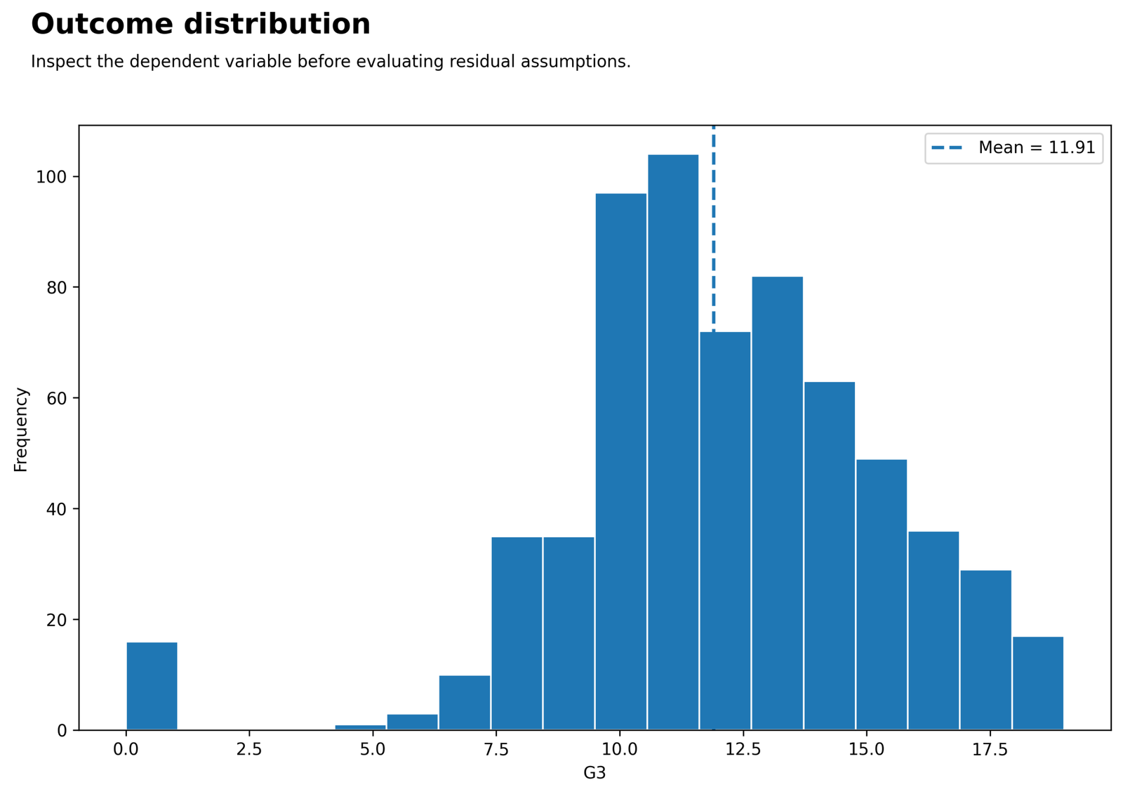
The outcome is bounded and concentrated in the middle, with a small group at zero.
G3 ranges from 0 to 19, with 649 observations.
The outcome distribution is not itself a regression assumption, but it explains why floor observations later generate extreme negative residuals.
Always distinguish the distribution of Y from the distribution of residuals after conditioning on predictors.
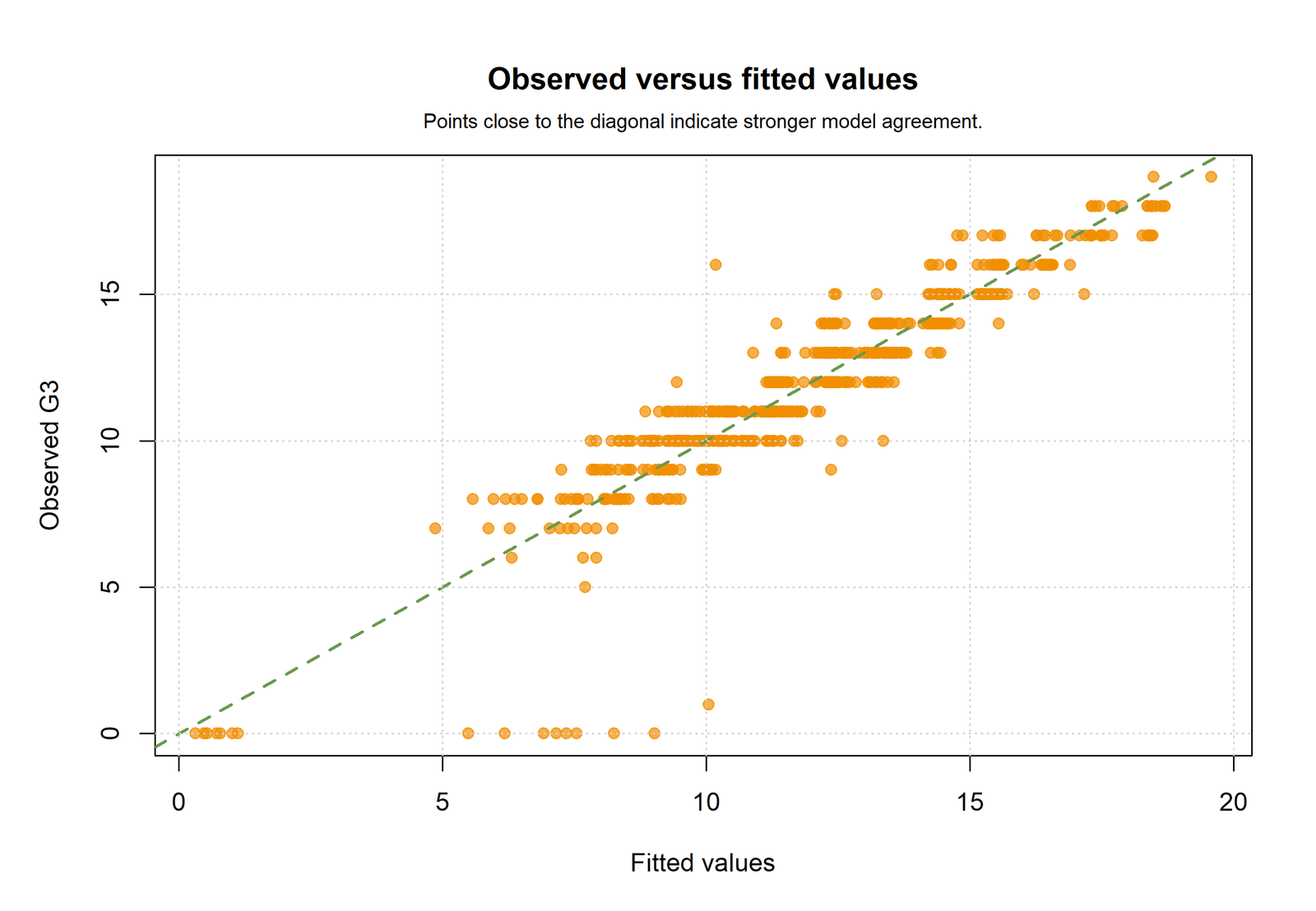
Python Chart 2: Observed Versus Fitted Values
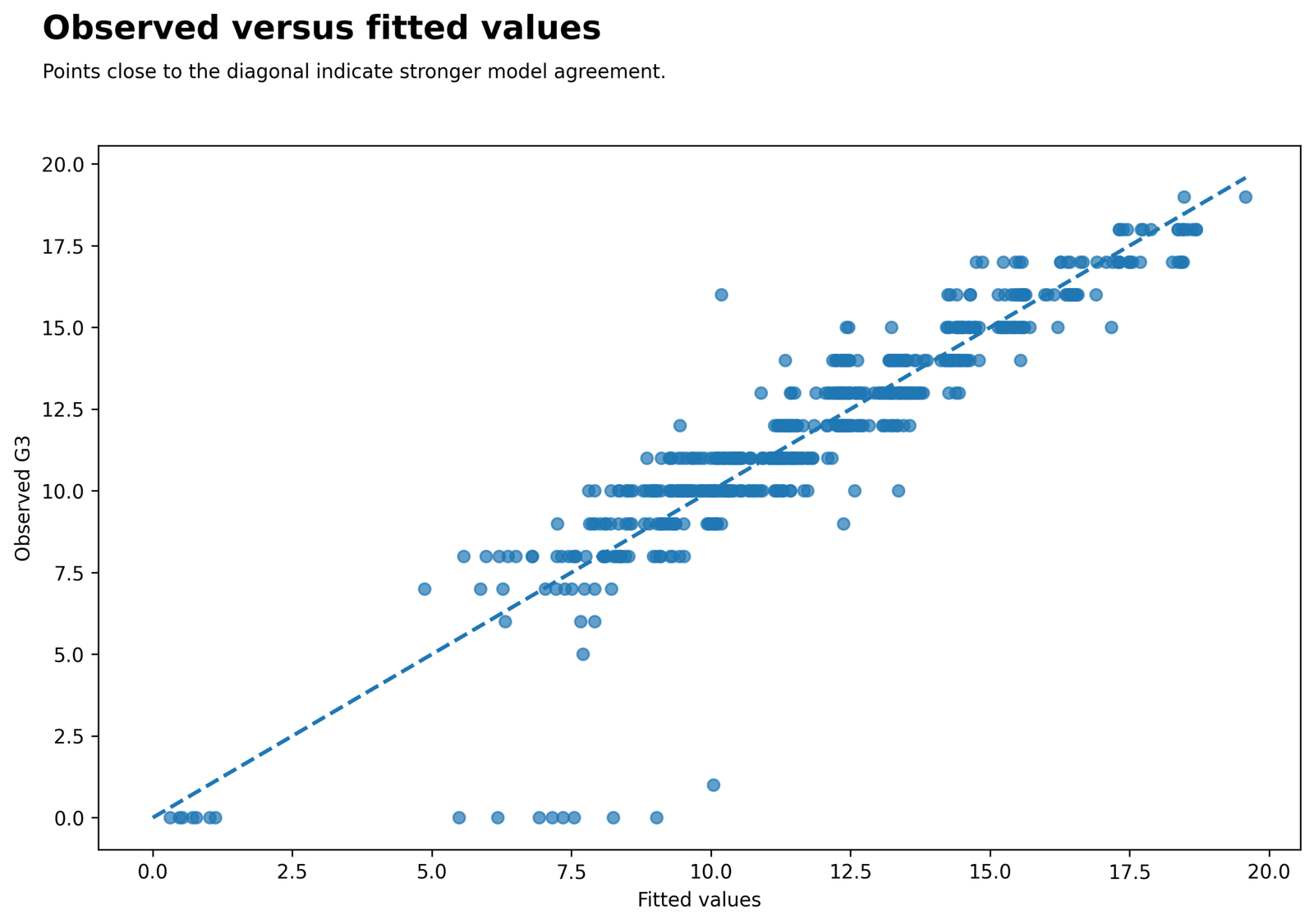
Most cases follow the diagonal, while several zero or very low outcomes sit far below their predictions.
R² = 0.850632, adjusted R² = 0.849236, RMSE = 1.254409.
The model captures the dominant outcome pattern, but strong fit coexists with a small set of severe errors.
Observed-versus-fitted agreement cannot prove linearity or homoscedasticity; it provides context for later diagnostics.
Python Chart 3: Residuals Versus Fitted Values
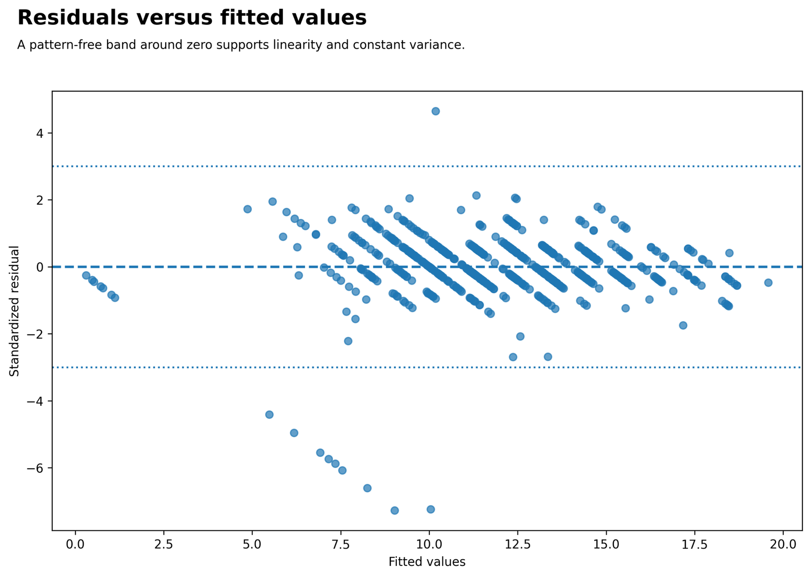
The residual cloud is centered near zero but shows changing structure and extreme negative cases.
RESET p = 0.001085; Breusch-Pagan p = 0.000010.
The plot and formal tests jointly suggest that the current additive linear specification and constant-variance assumption are incomplete.
A remedy may require nonlinear terms, interactions, robust covariance, or a different variance model rather than simply deleting residual outliers.
Python Chart 4: Scale-Location Plot
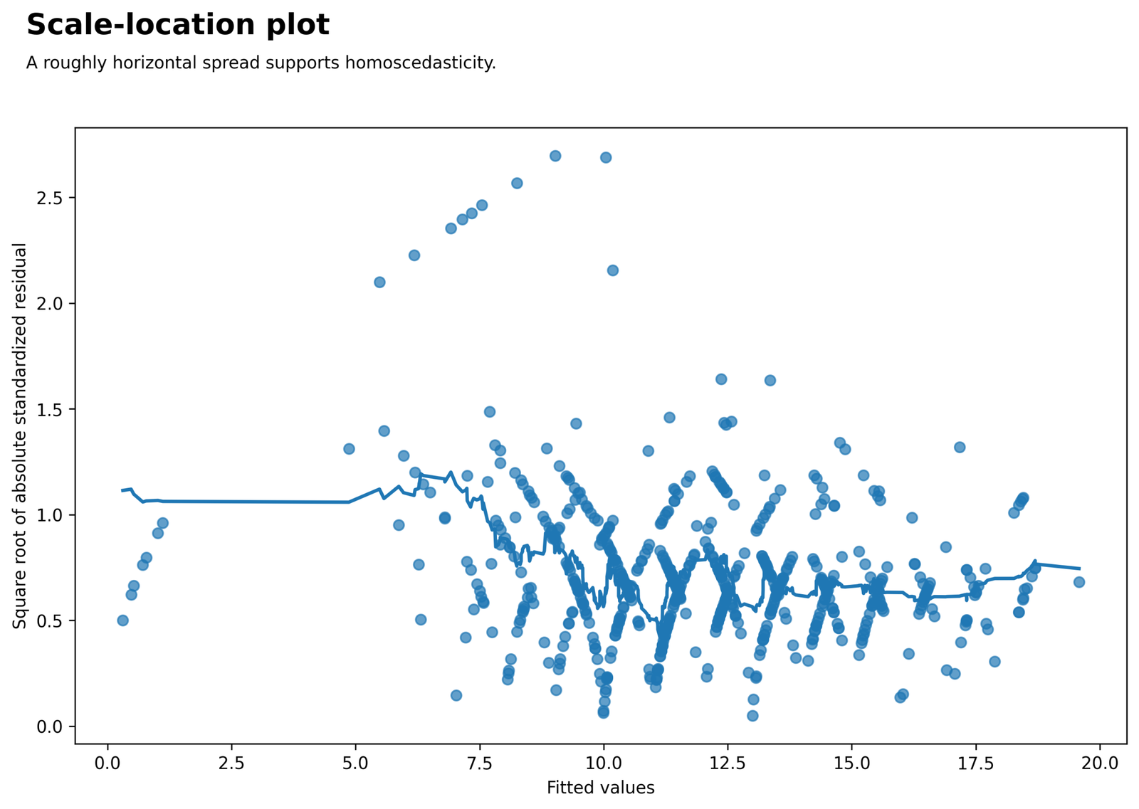
The smoothed square-root absolute residual pattern changes across fitted values instead of remaining flat.
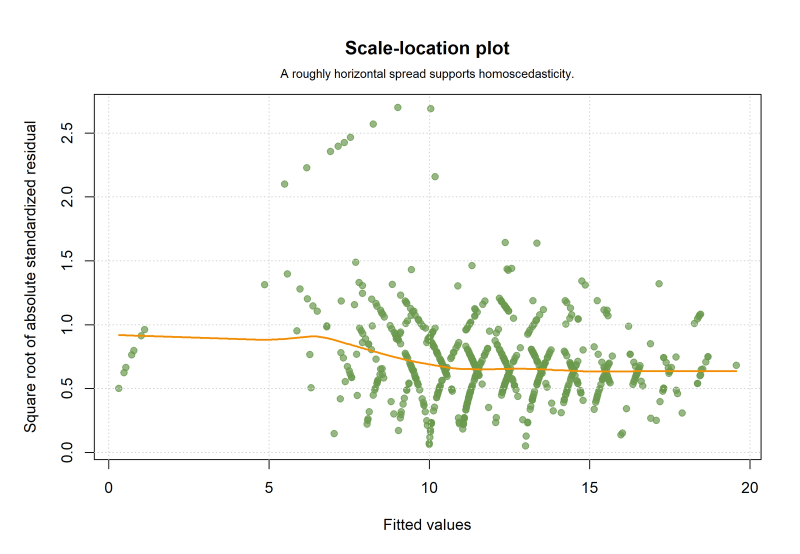
Correlation between fitted values and |residuals| = −0.209645, p < .001; White p = 0.00000175.
Residual spread is not constant. The negative correlation indicates larger absolute errors toward lower fitted values in this dataset.
The direction of heteroskedasticity guides whether transformation, robust standard errors, or weighted modeling is sensible.
Python Chart 5: Residual Histogram
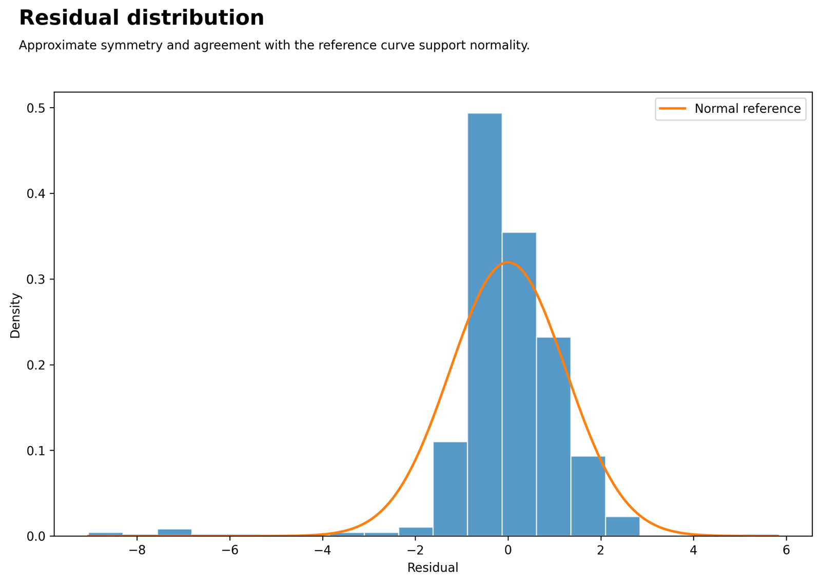
Most errors cluster near zero, but a long negative tail produces substantial asymmetry and kurtosis.
Shapiro-Wilk W = 0.754697; Jarque-Bera = 10152.729452.
The central mass is compact, but several extreme overpredictions make the residual distribution strongly non-normal.
The histogram shows what the normality tests detect and prevents a tiny p-value from being interpreted without shape information.
Python Chart 6: Residual Q-Q Plot
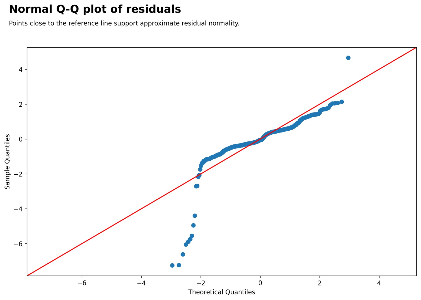
Central points are closer to the line, while tail observations diverge sharply, especially in the lower tail.
Maximum |externally studentized residual| = 7.590715; 10 cases exceed 3.
Normality failure is driven primarily by extreme tails rather than a uniform mismatch across all quantiles.
Robust inference and case sensitivity are more relevant than forcing perfect normality through arbitrary deletion.
Python Chart 7: Residual Sequence
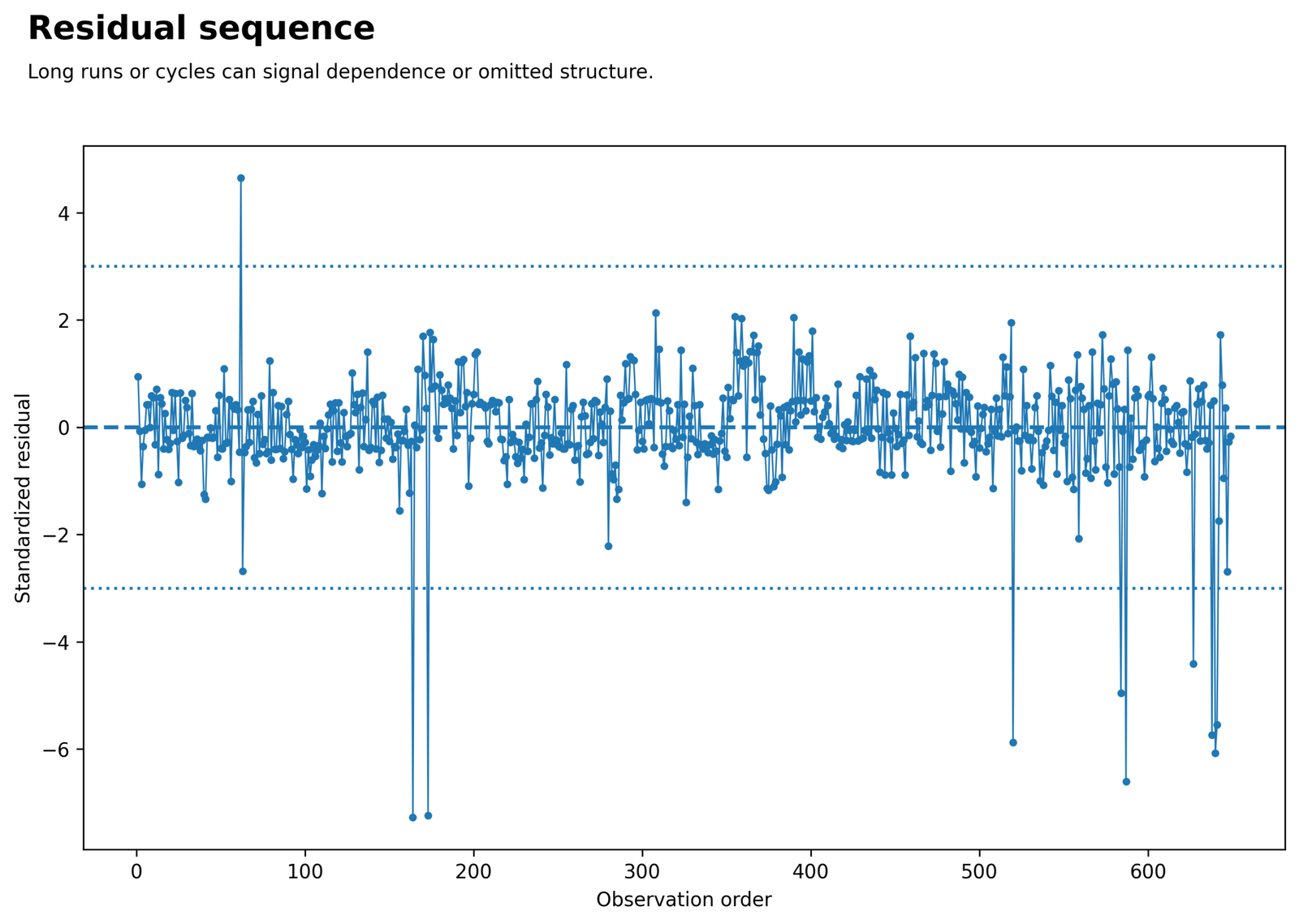
Residuals fluctuate around zero with isolated spikes and no dominant long drift.
Durbin-Watson = 1.860956.
There is no strong evidence of first-order autocorrelation in the supplied order, but independence still depends on the sampling design.
A Durbin-Watson result cannot detect every form of clustering and is meaningful only when row order represents a real sequence.
Python Chart 8: VIF Profile
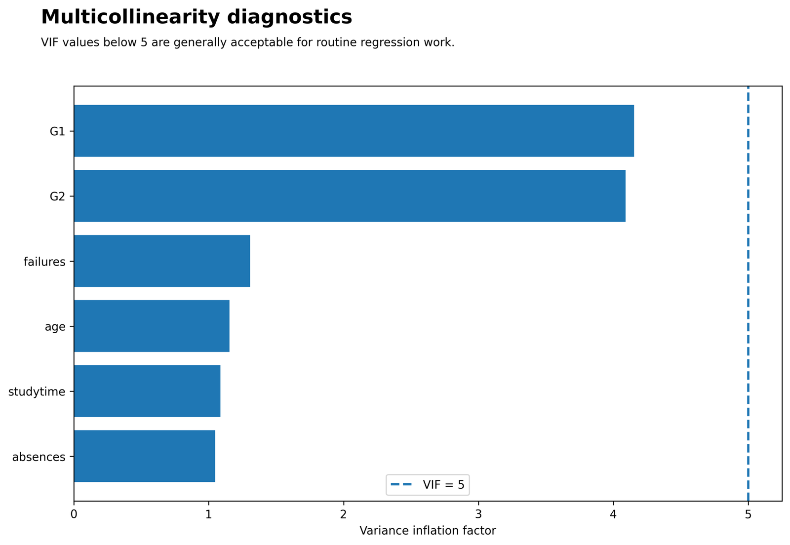
G1 and G2 have the largest VIF values, while the other predictors remain close to 1.
G1 VIF = 4.154857; G2 = 4.091388; all others are below 1.31.
Prior grades share substantial information, but the selected VIF < 5 guideline is not exceeded.
Moderate overlap can still affect individual coefficient precision even when it does not constitute a severe collinearity failure.
Python Chart 9: Cook’s Distance Across Cases
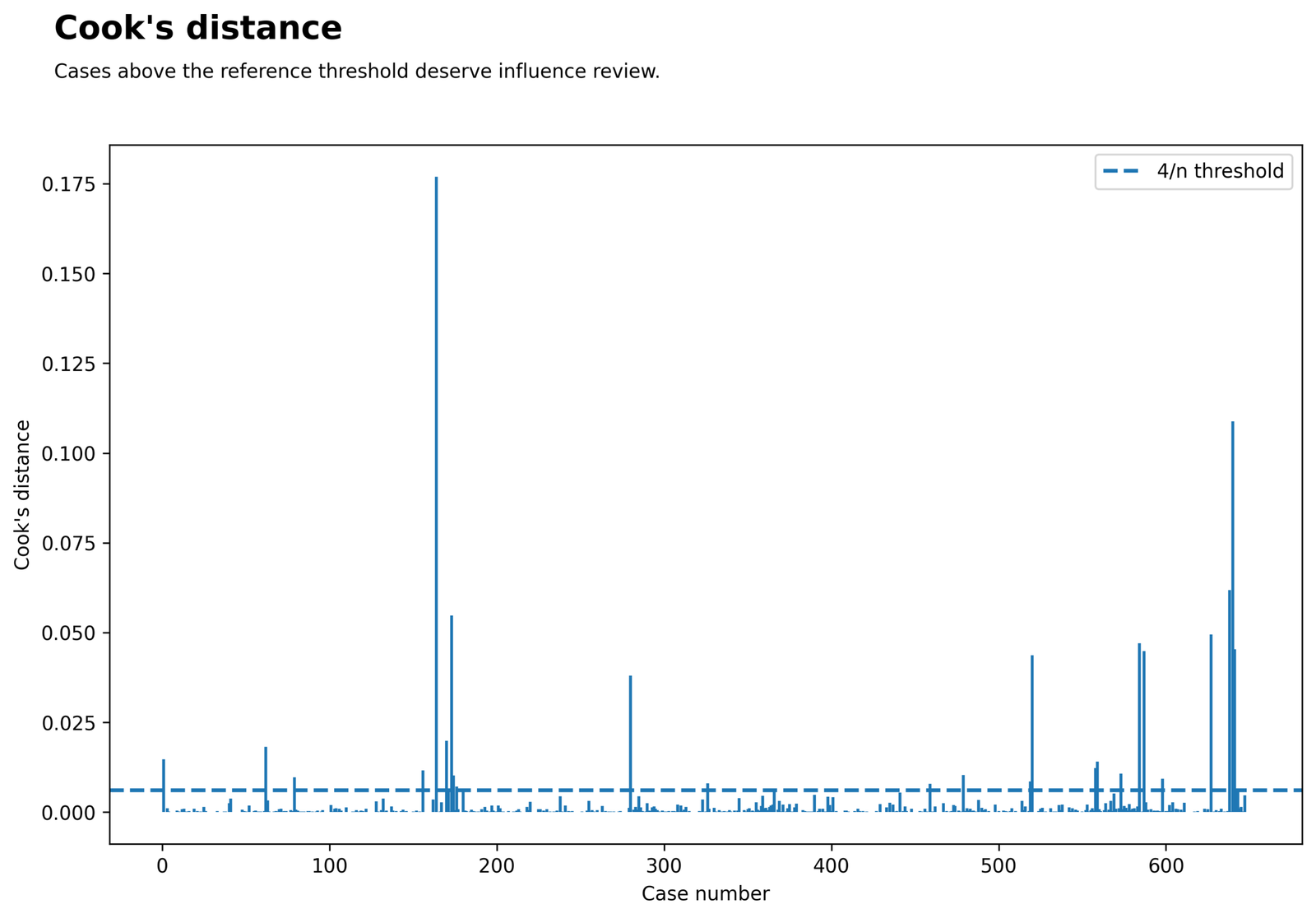
Most cases have negligible Cook’s distance, while a small set rises above the 4/n guideline.
Threshold = 0.00616333; 26 cases exceed it; maximum = 0.176952.
A limited group has enough residual-leverage combination to affect the fitted equation materially.
Refit the model without the most influential cases as a sensitivity analysis, then explain why estimates do or do not change.
Python Chart 10: Leverage and Studentized Residuals
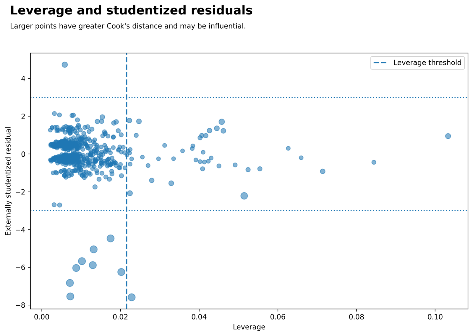
The joint plot separates unusual predictor profiles from unusual outcome errors and highlights cases high on both dimensions.
Leverage threshold = 0.02157165; 45 cases exceed it; 58 cases trigger at least one rule.
High leverage alone is not an error. Cases become most concerning when high leverage combines with a large studentized residual or large Cook’s distance.
The joint screen supports targeted case review instead of treating every flagged record as equally problematic.
R Charts and Explanations
The R figures verify the same outcome, fit, functional-form, and variance conclusions found in Python. The R figures reproduce the same Regression Assumptions conclusions using the supplied model.
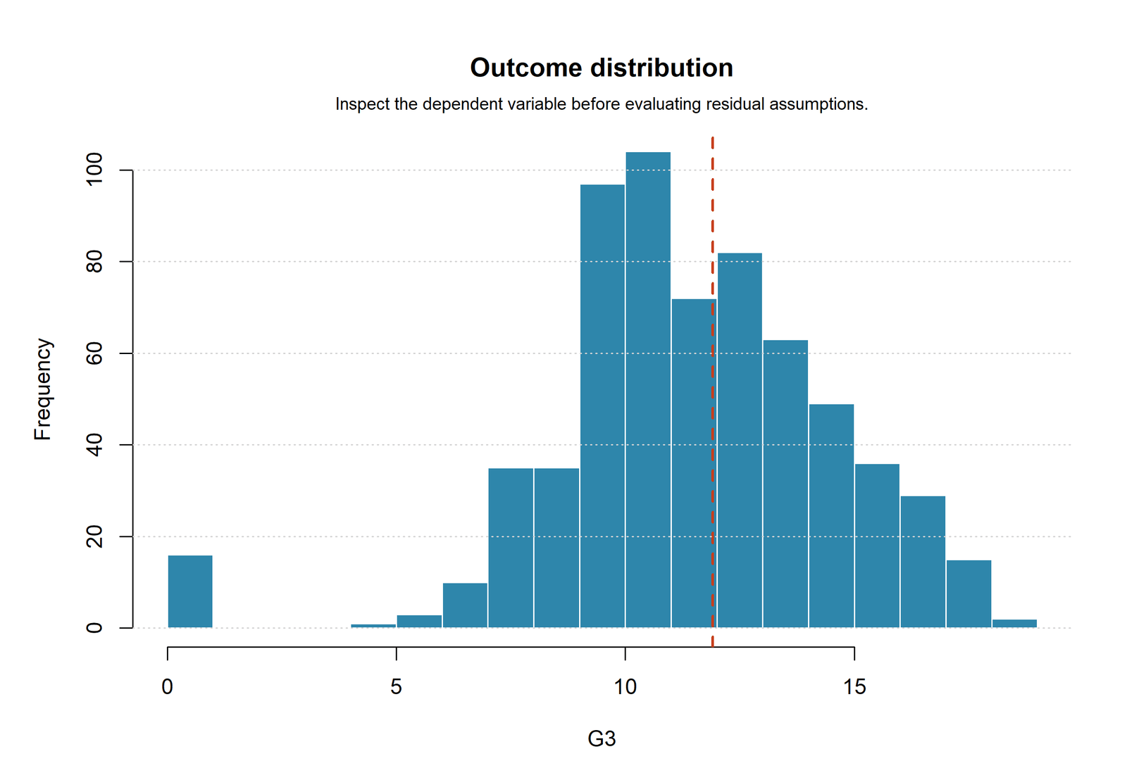
R Outcome Distribution
The bounded grade scale and zero outcomes provide context for the strong lower residual tail. This is descriptive evidence rather than an assumption test.
R Observed Versus Fitted Values
Most cases align well with predictions, confirming strong overall fit, while a small group of low outcomes remains far from the agreement line.
R Residuals Versus Fitted Values
The residual pattern, RESET result, and Breusch-Pagan result jointly indicate that the current mean and variance specifications need qualification.
R Scale-Location Plot
The smooth pattern is not horizontal, consistent with the significant White test and fitted-versus-absolute-residual correlation.
Condition-by-Condition Interpretation
Functional Form
The RESET result challenges the stated additive linear form. This does not mean the complete model is useless. It means fitted values contain systematic information not captured by the original predictor function. Candidate remedies may include a theory-supported G2 polynomial, interactions, transformations or a more flexible model. Regression Assumptions warnings should be translated into specific analytical consequences.
A Polynomial Regression term should not be added solely because RESET is significant. The altered model must be interpretable, validated and compared with the original.
Constant Variance
Breusch-Pagan, White and the scale-location pattern agree that residual variance changes with fitted values. Conventional OLS coefficients remain the same under robust covariance, but standard errors, confidence intervals and p-values may change.
HC3 robust standard errors are often a useful sensitivity analysis when leverage and unequal variance are both concerns. A transformation may also be considered when it matches the scientific scale and improves the conditional mean.
Residual Normality
Shapiro-Wilk and Jarque-Bera reject normality strongly. The plots show that the concern is concentrated in the tails, especially zero outcomes with predicted grades near the middle of the scale. Bootstrapping, robust uncertainty and influence sensitivity can supplement normal-theory results.
Independence
Durbin-Watson near 2 is supportive for first-order dependence in the supplied row order. It cannot detect every form of correlation. If students are nested within schools or classes, cluster-aware standard errors or multilevel models may still be necessary.
Multicollinearity
G1 and G2 are closely related but remain below the chosen VIF threshold. Their individual coefficients may be less stable than the overall prediction. Removing either variable solely to reduce VIF could omit important prior-grade information and change the estimand.
Outliers and Influence
Ten observations have externally studentized residuals beyond ±3, 45 have high leverage, 26 exceed the Cook’s distance rule, and 26 exceed the DFFITS rule. The union contains 58 observations.
These counts do not imply that 58 observations are erroneous. Each flag identifies a reason for closer examination. Sensitivity analysis should compare coefficients, uncertainty and predictions with influential cases retained, checked and, only where justified, excluded.
Influential Cases and Sensitivity Analysis
Highest Cook’s Distance Cases
| Case | Observed G3 | G1 | G2 | Fitted G3 | Raw residual | Externally studentized residual | Leverage | Cook’s D | DFFITS |
|---|---|---|---|---|---|---|---|---|---|
| 164 | 0 | 11 | 9 | 9.022936 | −9.022936 | −7.590715 | 0.022859 | 0.176952 | −1.160994 |
| 640 | 0 | 5 | 8 | 7.543323 | −7.543323 | −6.252879 | 0.020231 | 0.108871 | −0.898512 |
| 638 | 0 | 7 | 7 | 7.153776 | −7.153776 | −5.888928 | 0.012981 | 0.061908 | −0.675347 |
| 173 | 1 | 10 | 10 | 10.044619 | −9.044619 | −7.545231 | 0.007263 | 0.054732 | −0.645369 |
| 627 | 0 | 7 | 5 | 5.481558 | −5.481558 | −4.473388 | 0.017505 | 0.049468 | −0.597102 |
| 584 | 0 | 8 | 6 | 6.179390 | −6.179390 | −5.052835 | 0.013203 | 0.047002 | −0.584455 |
| 641 | 0 | 7 | 7 | 6.920620 | −6.920620 | −5.678819 | 0.010225 | 0.045386 | −0.577207 |
| 587 | 0 | 8 | 8 | 8.250282 | −8.250282 | −6.831440 | 0.007161 | 0.044893 | −0.580174 |
| 520 | 0 | 8 | 7 | 7.343242 | −7.343242 | −6.040059 | 0.008762 | 0.043656 | −0.567873 |
| 280 | 5 | 7 | 8 | 7.704422 | −2.704422 | −2.220417 | 0.051467 | 0.037984 | −0.517219 |
Highest-Leverage Cases
Case 1 has maximum leverage of 0.103309 because G1 = 0 creates an unusual predictor profile, but its externally studentized residual is only 0.944918. Case 611 has leverage 0.084443, and cases 598, 198 and 213 also have leverage above 0.06. High leverage alone does not mean the observed outcome is poorly fitted. Regression Assumptions case flags are screening tools rather than deletion commands.
Recommended Sensitivity Sequence
- Verify source values, coding and outcome status for every extreme case.
- Refit the original model with HC3 robust standard errors.
- Compare coefficients with and without the highest Cook’s distance cases, while reporting both analyses.
- Evaluate a theory-supported alternative mean function.
- Recalculate every Regression Assumptions diagnostic for the revised specification.
- Explain whether conclusions change materially or only numerically.
Regression Assumptions, Consequences and Remedies
| Condition | Current evidence | Main consequence | Reasonable response |
|---|---|---|---|
| Functional form | RESET p = .001085 | Biased conditional mean or systematic residual pattern | Test theory-based nonlinear terms, interactions, splines, or alternative specification |
| Homoscedasticity | BP and White p < .001 | Conventional SEs may be wrong | Robust covariance, transformation, weighted or generalized least squares |
| Residual normality | Shapiro and JB reject; tail departures visible | Exact small-sample intervals/tests affected | Robust or bootstrap inference; inspect influential cases |
| Independence | DW = 1.861 | No strong first-order autocorrelation detected | Still verify clustering from design |
| Multicollinearity | Maximum VIF = 4.155 | Moderate precision inflation for G1/G2 | Retain if theoretically needed; report conditional effects |
| Influence | 58 cases trigger a rule | Potential sensitivity of coefficients and predictions | Case review and sensitivity refits |
Robust Standard Errors
HC3 or another heteroskedasticity-consistent covariance estimator can be reported when the linear coefficient estimand remains useful. Robust standard errors do not repair omitted nonlinear structure; they address uncertainty under unequal variance. Every Regression Assumptions remedy requires a fresh diagnostic audit.
Transformations
Transformations can change variance and functional form together, but they also change interpretation. Select them because they produce a scientifically meaningful scale, not only because a test p-value becomes larger.
Weighted and Generalized Least Squares
When residual variance can be modeled from predictors or fitted values, weighted least squares or GLS may improve efficiency. Incorrect weights can worsen results, so the variance model needs validation.
Robust Regression
Robust Regression reduces the impact of extreme residuals, but it answers a somewhat different fitting question from OLS. Compare conclusions rather than silently replacing the original model.
Model Respecification
RESET evidence supports investigating nonlinear and interaction terms. Respecification should avoid data-driven overfitting and preserve hierarchical principles.
Regression Assumptions in Python, R, SPSS and Excel
Python
Statsmodels and SciPy support residual tests, VIF, influence measures, robust covariance, and diagnostic plots. Regression Assumptions comparisons require identical models and definitions across software.
- RESET, Breusch-Pagan, White, Jarque-Bera
- Durbin-Watson and VIF
- Externally studentized residuals
- Leverage, Cook’s distance, DFFITS
R
R combines lm(), diagnostic plots, car, lmtest, and influence functions for a reproducible audit.
resettest()bptest()vif()influence.measures()
SPSS
SPSS REGRESSION can save residuals, leverage, Cook’s distance, and predicted values. Additional diagnostics can be produced through plots, collinearity statistics, and supported extensions.
Excel
Excel can calculate residuals, standardized residuals, VIF support regressions, thresholds, and influence flags. Specialized software remains preferable for externally studentized residuals and formal tests.
Code: Expand Only the Software You Need
Python Regression Assumptions code
import pandas as pd
import statsmodels.api as sm
from scipy import stats
from statsmodels.stats.diagnostic import (
    linear_reset, het_breuschpagan, het_white
)
from statsmodels.stats.outliers_influence import (
    OLSInfluence, variance_inflation_factor
)
from statsmodels.stats.stattools import durbin_watson, jarque_bera

df = pd.read_csv("dataset.csv")
cols = ["G3","G1","G2","studytime","failures","absences","age"]
work = df[cols].dropna().copy()

y = work["G3"].astype(float)
X = sm.add_constant(work[cols[1:]].astype(float))
model = sm.OLS(y, X).fit()

reset = linear_reset(model, power=2, use_f=True)
bp = het_breuschpagan(model.resid, model.model.exog)
white = het_white(model.resid, model.model.exog)
shapiro = stats.shapiro(model.resid)
jb = jarque_bera(model.resid)
dw = durbin_watson(model.resid)

influence = OLSInfluence(model)
studentized = influence.resid_studentized_external
leverage = influence.hat_matrix_diag
cooks_d = influence.cooks_distance[0]
dffits = influence.dffits[0]

print(model.summary())
print("RESET:", reset.fvalue, reset.pvalue)
print("Breusch-Pagan:", bp)
print("White:", white)
print("Shapiro:", shapiro)
print("Jarque-Bera:", jb)
print("Durbin-Watson:", dw)
R Regression Assumptions code
df <- read.csv("dataset.csv")
work <- na.omit(df[c(
  "G3","G1","G2","studytime","failures","absences","age"
)])

model <- lm(
  G3 ~ G1 + G2 + studytime + failures + absences + age,
  data = work
)

summary(model)
par(mfrow = c(2, 2))
plot(model)

library(lmtest)
library(car)

resettest(model, power = 2, type = "fitted")
bptest(model)
durbinWatsonTest(model)
vif(model)

shapiro.test(residuals(model))
cooks.distance(model)
hatvalues(model)
rstudent(model)
dffits(model)
SPSS Regression Assumptions syntax
REGRESSION
 /DEPENDENT G3
 /METHOD=ENTER G1 G2 studytime failures absences age
 /STATISTICS COEFF OUTS R ANOVA CI(95) COLLIN TOL
 /RESIDUALS HISTOGRAM(ZRESID) NORMPROB(ZRESID)
 /SCATTERPLOT=(*ZPRED,*ZRESID)
 /SAVE PRED(PRED_G3)
       RESID(RESID_G3)
       SRESID(SRESID_G3)
       SDRESID(SDRESID_G3)
       LEVER(LEV_G3)
       COOK(COOK_G3).

OUTPUT EXPORT
 /CONTENTS EXPORT=ALL LAYERS=PRINTSETTING MODELVIEWS=PRINTSETTING
 /PDF DOCUMENTFILE=
'D:\DATA ANALYSIS\H Regression Tests and Models\Regression Assumptions\SPSS_Output\pdf\Regression-Assumptions-SPSS-Output.pdf'.
Excel diagnostic formulas
Raw residual:
=Observed_G3-Predicted_G3

Standardized residual:
=Residual/RMSE

Leverage guideline:
=2*(Predictor_Count+1)/N

Cook's distance guideline:
=4/N

DFFITS guideline:
=2*SQRT((Predictor_Count+1)/N)

Tolerance:
=1-R_Squared_From_Auxiliary_Regression

VIF:
=1/Tolerance

Any influence flag:
=OR(
 ABS(Studentized_Residual)>3,
 Leverage>Leverage_Threshold,
 Cooks_Distance>Cooks_Threshold,
 ABS(DFFITS)>DFFITS_Threshold
)
[]
[]
[]
[]
[]
[]
[]
Advanced Regression Assumptions Topics
Regression Assumptions Overview
Regression Assumptions are separate model conditions. Each condition requires its own evidence, consequence and response. Regression Assumptions interpretation should remain tied to the declared model.
Linearity of the Conditional Mean
Linearity concerns whether the stated predictor function represents expected G3 adequately. A model can contain polynomial and interaction terms while remaining linear in coefficients. Regression Assumptions interpretation should remain tied to the declared model.
Ramsey RESET Test
The Ramsey RESET Test detects omitted functional structure through powers of fitted values. It does not reveal which term should be added. Regression Assumptions interpretation should remain tied to the declared model.
Residuals Versus Fitted Plot
A systematic smooth suggests mean misspecification. A changing vertical spread suggests unequal variance. Individual distant points suggest case review. Regression Assumptions interpretation should remain tied to the declared model.
Additivity
Additivity assumes predictor contributions combine without omitted interactions. Subject-matter theory should determine which interactions are plausible. Regression Assumptions interpretation should remain tied to the declared model.
Interaction Effects
Interactions change the effect of one predictor across another predictor. They should be explained with predicted values rather than coefficient signs alone. Regression Assumptions interpretation should remain tied to the declared model.
Homoscedasticity
Homoscedasticity means conditional residual variance is stable. Violation mainly affects conventional uncertainty, not the numerical ability to calculate OLS coefficients. Regression Assumptions interpretation should remain tied to the declared model.
Breusch-Pagan Test
The Breusch-Pagan Test evaluates whether residual variance is associated with the predictor design. Regression Assumptions interpretation should remain tied to the declared model.
White Test
The White Test provides a broader variance-specification check that can capture nonlinear variance patterns. Regression Assumptions interpretation should remain tied to the declared model.
Robust Standard Errors
HC3 robust covariance is especially relevant when leverage and unequal variance occur together. Coefficients remain unchanged while uncertainty is recalculated. Regression Assumptions interpretation should remain tied to the declared model.
Residual Normality
Normality supports exact small-sample t and F reference distributions. Large samples provide some protection, but severe tails still affect influence and uncertainty. Regression Assumptions interpretation should remain tied to the declared model.
Shapiro-Wilk Test
The Shapiro-Wilk Test is sensitive to departures from normality and should be interpreted with the histogram and Q-Q plot. Regression Assumptions interpretation should remain tied to the declared model.
Jarque-Bera Test
The Jarque-Bera Test combines residual skewness and kurtosis into a distribution-shape diagnostic. Regression Assumptions interpretation should remain tied to the declared model.
Q-Q Plot
A Q-Q plot reveals whether departures occur through the complete distribution or are concentrated in one or both tails. Regression Assumptions interpretation should remain tied to the declared model.
Independence of Errors
Independence follows from design and sampling. Residual-order diagnostics cannot rule out school, class or subject clustering. Regression Assumptions interpretation should remain tied to the declared model.
Durbin-Watson Statistic
The Durbin-Watson Test targets first-order autocorrelation when record order represents a meaningful sequence. Regression Assumptions interpretation should remain tied to the declared model.
Clustered Observations
Clustered observations require cluster-robust, generalized estimating equation or multilevel methods even when Durbin-Watson is near 2. Regression Assumptions interpretation should remain tied to the declared model.
Variance Inflation Factor
Variance Inflation Factor measures how strongly one predictor is explained by the remaining predictors and how much its coefficient variance is inflated. Regression Assumptions interpretation should remain tied to the declared model.
Tolerance
Tolerance Statistic equals 1/VIF and describes the predictor variation remaining after the other predictors are considered. Regression Assumptions interpretation should remain tied to the declared model.
Condition Number
The scaled condition number evaluates numerical dependence in the complete design matrix and complements predictor-specific VIF values. Regression Assumptions interpretation should remain tied to the declared model.
Leverage
Leverage measures how unusual a predictor profile is. A high-leverage case can have either a small or large residual. Regression Assumptions interpretation should remain tied to the declared model.
Externally Studentized Residuals
Studentized Residuals scale errors for residual variance and leverage. External studentization leaves the case out of the variance estimate. Regression Assumptions interpretation should remain tied to the declared model.
Cook’s Distance
Cook’s Distance combines residual magnitude and leverage to screen for cases that may alter the fitted equation. Regression Assumptions interpretation should remain tied to the declared model.
DFFITS
DFFITS measures the standardized change in a case’s fitted value when that observation is removed. Regression Assumptions interpretation should remain tied to the declared model.
Influence Sensitivity Analysis
Compare the original coefficients and conclusions with transparent refits that address the most influential cases. Do not present automatic deletion as a remedy. Regression Assumptions interpretation should remain tied to the declared model.
Reporting Regression Assumptions
State the diagnostic, statistic, threshold or p-value, visible pattern, consequence, and analytical response for each condition. Regression Assumptions interpretation should remain tied to the declared model.
APA-Style Reporting
Functional form was challenged by Ramsey RESET, F = 10.77, p = .001. Heteroskedasticity was indicated by the Breusch-Pagan test, LM = 33.05, p < .001, and the White test, LM = 75.55, p < .001.
Residual normality was rejected, Shapiro-Wilk W = .755, p < .001, and Jarque-Bera = 10152.73, p < .001. Durbin-Watson was 1.86, providing no strong evidence of first-order autocorrelation in the supplied record order.
The largest VIF was 4.15 for G1, followed by 4.09 for G2. Influence screening identified 10 residual outliers, 45 high-leverage observations, 26 cases above the Cook’s distance rule and 26 above the DFFITS rule; 58 observations met at least one rule.
Regression Assumptions findings therefore supported reporting heteroskedasticity-robust uncertainty, a theory-led functional-form comparison and influential-case sensitivity analysis.
Publication Checklist
Include
- Outcome, predictors, sample size and estimator
- Residual-versus-fitted and scale-location plots
- RESET, Breusch-Pagan and White results
- Histogram, Q-Q plot and normality evidence
- Independence rationale and Durbin-Watson where appropriate
- VIF, tolerance and condition number
- Studentized residual, leverage, Cook’s distance and DFFITS rules
- Robust and influence sensitivity analyses
Avoid
- One universal pass-or-fail conclusion
- Calling R² a Regression Assumptions test
- Testing outcome normality instead of residual behavior
- Treating VIF 5 as a universal law
- Calling Durbin-Watson proof of complete independence
- Deleting every flagged observation
- Changing the equation only to improve plots
- Reporting formal tests without practical consequences
Connect Regression Assumptions p-values to P-Value, uncertainty to Confidence Interval and Standard Error, and substantive magnitude to Effect Size.
Downloads
Regression Assumptions R ReportR model diagnostics and four supplied chart explanations
Regression Assumptions SPSS OutputSPSS regression, collinearity, residual and casewise output
Regression Assumptions Worked ExcelCase-level residuals, leverage, Cook’s distance, DFFITS and Boolean flags
Frequently Asked Questions
What are Regression Assumptions?
Regression Assumptions are model-specific conditions concerning functional form, residual variance, dependence, predictor geometry, distribution shape and influential observations. Regression Assumptions conclusions should remain condition-specific.
Did every condition pass?
No. Functional form, constant variance and residual normality are challenged. The selected collinearity guidelines and first-order residual-order check are reasonably supported. Regression Assumptions conclusions should remain condition-specific.
Does high R-squared prove the assumptions are met?
No. R-squared measures sample variation explained and does not test form, variance, normality, independence or influence. Regression Assumptions conclusions should remain condition-specific.
What does the significant RESET result mean?
It suggests omitted mean structure but does not identify the correct polynomial, interaction or transformation. Regression Assumptions conclusions should remain condition-specific.
What should be done about heteroskedasticity?
Use suitable robust standard errors, review the mean specification and consider a scientifically meaningful variance or transformation model. Regression Assumptions conclusions should remain condition-specific.
Do non-normal residuals invalidate OLS coefficients?
Not automatically. Point estimates may remain useful, but exact normal-theory inference and tail-sensitive conclusions need qualification. Regression Assumptions conclusions should remain condition-specific.
Is Durbin-Watson 1.86 acceptable?
It is close to 2 and does not indicate strong first-order autocorrelation in the supplied order, but independence still depends on design. Regression Assumptions conclusions should remain condition-specific.
Are G1 and G2 too collinear?
Their VIF values are approximately 4.15 and 4.09. They share substantial information but remain below the selected threshold of 5. Regression Assumptions conclusions should remain condition-specific.
What is the leverage threshold?
The selected rule is 2(p + 1)/n = 0.02157165. Forty-five cases exceed it. Regression Assumptions conclusions should remain condition-specific.
What is the Cook’s distance threshold?
The selected 4/n guideline is 0.00616333. Twenty-six cases exceed it. Regression Assumptions conclusions should remain condition-specific.
How many residual outliers were found?
Ten observations have absolute externally studentized residuals greater than 3. Regression Assumptions conclusions should remain condition-specific.
Should all 58 flagged cases be deleted?
No. A flag requests verification and sensitivity analysis. Automatic deletion can bias the sample. Regression Assumptions conclusions should remain condition-specific.
What is the most influential case?
Case 164 has Cook’s distance 0.176952, externally studentized residual −7.590715 and DFFITS −1.160994. Regression Assumptions conclusions should remain condition-specific.
Why is case 1 important?
Case 1 has maximum leverage of 0.103309 but a moderate residual, illustrating that leverage and outlyingness are different. Regression Assumptions conclusions should remain condition-specific.
Can Regression Assumptions be checked in Excel?
Excel can audit formulas and flags, but Python, R or SPSS is preferable for formal tests and matrix-based influence measures. Regression Assumptions conclusions should remain condition-specific.
How should Regression Assumptions be reported?
Report every condition separately with its diagnostic evidence, consequence and any robust or sensitivity analysis performed. Regression Assumptions conclusions should remain condition-specific.
Regression Assumptions Conclusion
The Regression Assumptions audit produces a mixed result. The six-predictor model explains approximately 85.06% of G3 variation and does not show severe multicollinearity or strong first-order residual autocorrelation under the selected rules.
Ramsey RESET challenges the stated functional form, Breusch-Pagan and White tests challenge constant variance, and residual normality tests reveal severe tail departures. Influence screening identifies a smaller group of cases with large errors, unusual predictor profiles or both.
The appropriate response is not to discard the model or remove every flagged observation. The original equation should remain a transparent baseline, conventional inference should be compared with robust inference, a limited theory-led alternative form should be evaluated, and influence sensitivity should be documented.

