
Count-model dispersion and Pearson-scaled uncertainty
Quasi Poisson Regression: Formula, Interpretation, SPSS, Python, R and Excel Guide
Learn how Quasi Poisson Regression separates a Poisson log-linked mean from its variance scale, how dispersion changes standard errors without changing fitted counts, and how to interpret the complete worked analysis in Python, R, SPSS and Excel.
Pearson dispersion: 0.243139
Outcome: count_outcome from G3
Python, R, SPSS and Excel
Quasi Poisson Regression Model Overview
Quasi Poisson Regression is a generalized linear modeling approach for nonnegative count-like outcomes when the ordinary Poisson variance assumption is too restrictive. The model keeps the familiar log-linked mean, log(μi) = xi′β, but replaces the fixed equality Var(Yi|Xi) = μi with Var(Yi|Xi) = φμi. The parameter φ is a dispersion multiplier estimated from the residual evidence. Values above one indicate overdispersion, values near one support the ordinary Poisson benchmark, and values below one indicate underdispersion.
The central research question is not simply whether predictors are associated with the outcome. It is whether the multiplicative mean relationships estimated by a Poisson log-link remain interpretable when uncertainty is calculated from an estimated variance scale rather than from a unit-dispersion assumption. Quasi Poisson Regression is therefore especially useful when the mean equation appears reasonable but residual variation is systematically greater or smaller than the Poisson model expects.
Use Quasi Poisson Regression when the response is nonnegative and count-like, observations are independent for the displayed covariance calculation, the logarithmic mean relationship is appropriate, and residual variance is reasonably proportional to the fitted mean through one common φ. It is frequently introduced for overdispersed event counts, but the method also supports underdispersion. The present analysis is an important example because φ̂ = 0.243139, far below one.
Do not use Quasi Poisson Regression merely because a Poisson p-value is inconvenient. It is also not the first choice when the response contains a separate structural-zero process, when observations are clustered or repeated without a dependence model, when a full probability likelihood is required for ordinary AIC or likelihood-ratio testing, or when the scientific outcome is better represented as continuous, ordinal, binomial, or bounded. For these situations, compare Zero-Inflated Poisson Regression, Hurdle Regression, Generalized Estimating Equations, or Multilevel Regression.
Compared with Poisson Regression, Quasi Poisson Regression estimates the same conditional mean when the formula, data, link, weights and offset are unchanged. It modifies the covariance matrix through φ. Compared with Negative Binomial Regression, it does not specify a full probability mass function and does not impose the usual quadratic overdispersion pattern. Compared with a robust sandwich covariance, it makes the more specific proportional-variance assumption φμ.
The coefficients remain log rate ratios. A numeric coefficient βj becomes exp(βj), the multiplicative change in the fitted conditional mean for a one-unit predictor increase while the other variables remain fixed. A factor coefficient compares its displayed category with the reference category. Dispersion does not change those point estimates. It changes the standard error, confidence interval, test statistic and p-value used to describe their uncertainty.
Supported predictors include numeric variables, indicator variables, treatment-coded factors, interactions, nonlinear terms and offsets. The response should remain nonnegative and should have a mean interpretation compatible with the log link. The principal assumptions are a correctly specified conditional mean, a variance approximately proportional to μ through one global φ, independent observations for the model-based covariance, an estimable design matrix, adequate sample information and honest outcome measurement.
The main advantage of Quasi Poisson Regression is transparent variance correction without changing the fitted Poisson mean. It is easy to audit because the scale can be calculated directly from Pearson chi-square and residual degrees of freedom. Its limitations are equally important: no ordinary likelihood-based AIC, no automatic solution to clustering or zero inflation, no full predictive distribution, and sensitivity to mean-model misspecification.
In the worked scenario, 649 student records are modeled with an intercept, six numeric predictors—G1, G2, studytime, failures, absences and age—and three factor contrasts for school, sex and address. The engineered count outcome is derived from G3. Pearson chi-square is 155.365855 on 639 residual degrees of freedom, giving φ̂ = 0.243139. Because √φ̂ is about 0.493, scaled standard errors are roughly half their ordinary Poisson values. Coefficients, rate ratios and fitted counts remain unchanged.
Quick Answer
What Stayed Unchanged
- Every regression coefficient β
- Every rate ratio exp(β)
- The linear predictor and all fitted counts
- Residual deviance: 247.065469
- The substantive conditional-mean equation
What Changed After Scaling
- Model-based covariance multiplied by φ̂
- Standard errors multiplied by √φ̂ ≈ 0.493091
- Wald statistics and p-values
- Confidence-interval widths
- Several threshold-based significance decisions
The strongest positive predictor is G2. Its coefficient is 0.086381 and its rate ratio is 1.090222, meaning a one-point increase in G2 multiplies the adjusted fitted mean by about 1.090. Under Pearson scaling, the 95% rate-ratio interval is 1.080959 to 1.099563 and p = 1.25639 × 10−87.
The school contrast illustrates the inferential effect of underdispersion. Its rate ratio remains 0.967171. The ordinary Poisson p-value is 0.228159, but the scaled standard error is 0.013658, giving p = 0.014525 and a 95% rate-ratio interval of 0.941624 to 0.993411. This is a precision change, not a new coefficient.
Do not report the numeric scaled-GLM field 12316.663065 as a valid Quasi Poisson Regression AIC. A true quasi model lacks the complete likelihood required for ordinary AIC, and R correctly returns NA.
Table of Contents
- Model Overview
- Quick Answer
- When Quasi Poisson Regression Is Needed
- How Quasi Poisson Regression Works
- Variables and Data Dictionary
- Verified Results
- Python Chart Stories
- R Chart Pairs
- Coefficient Interpretation
- Predictions and Effects
- Assumptions and Diagnostics
- Python, R, SPSS and Excel
- Reproducible Code
- Advanced Topics
- APA-Style Reporting
- Publication Checklist
- Downloads
- Related Guides
- Frequently Asked Questions
- Conclusion
When Quasi Poisson Regression Is Needed
Ordinary Poisson regression assumes that the conditional variance equals the conditional mean. That equality is a strong claim about residual spread, not a requirement for the log-linked mean itself. Quasi Poisson Regression is needed when the mean equation remains useful but the unit-dispersion variance makes uncertainty too large or too small.
The worked response is bounded from 0 to 20, so unrestricted count variation is not possible. This compressed support helps explain why Pearson variation is smaller than residual degrees of freedom. Before selecting any count model, summarize the outcome with Descriptive Statistics, inspect its Frequency Distribution, and evaluate whether zeros, bounds and exposure have scientific meaning.
Quasi Poisson Regression is preferable to a simpler Poisson model when the dispersion evidence is strong and a proportional scale is defensible. It is preferable to a negative-binomial model when the observed variance is below the mean benchmark or when a full quadratic overdispersion structure is not required. It is not a substitute for revising a misspecified mean, adding a missing exposure offset, or modeling dependence.
Use Quasi Poisson Regression When
- The outcome is nonnegative and count-like.
- The log-linked mean is substantively meaningful.
- Dispersion differs from one.
- A single proportional φ is a reasonable summary.
- Rate ratios are the intended effect measure.
- Ordinary likelihood AIC is not essential.
Choose Another Method When
- Structural zeros require a mixture model.
- Repeated or clustered observations require correlation modeling.
- The outcome is fundamentally ordinal or continuous.
- A complete likelihood is required for the analysis plan.
- Variance is not approximately proportional to the mean.
- The log mean needs substantial functional-form revision.
How Quasi Poisson Regression Works
Use a log link so μi = exp(xi′β) remains positive.
Estimate the same β values produced by the corresponding Poisson mean model.
Calculate φ̂ from Pearson chi-square divided by residual degrees of freedom.
Multiply covariance by φ̂ and standard errors by √φ̂; then rebuild tests and intervals.
The Pearson residual for observation i is the raw residual divided by √μ̂i. Squaring and summing those residuals gives Pearson chi-square. The residual degrees of freedom subtract the estimated parameter count from the number of usable observations. This is why the denominator is 639 rather than 649.
Because φ is one scalar multiplier, it cancels from the estimating equation for β. The Quasi Poisson Regression coefficient vector therefore matches the ordinary Generalized Linear Model with Poisson family and log link. The variance estimate is applied to the normalized covariance after the shared mean has been fitted.
When φ̂ is below one, the scaled covariance is smaller. Here √φ̂ ≈ 0.493091. A standard error of 0.027699 for school MS becomes 0.013658 after rounding. The coefficient remains −0.033380 and the rate ratio remains 0.967171. The test statistic becomes larger in magnitude because the unchanged coefficient is divided by a smaller standard error.
Confidence intervals should be constructed on the coefficient scale and then exponentiated for rate-ratio reporting. Review the Confidence Interval, Standard Error and P-Value guides before interpreting threshold changes as substantive importance.
Variables and Data Dictionary
The Quasi Poisson Regression model uses all 649 records. The outcome is a rounded, nonnegative count-like version of G3. Six numeric predictors enter as one-unit linear terms, and three categorical predictors enter through treatment-coded contrasts. No exposure offset, sampling weight, interaction or nonlinear term is present.
| Variable | Role | Type and coding | Interpretation in the model |
|---|---|---|---|
| count_outcome | Outcome | Nonnegative G3-derived count, bounded 0–20 | Conditional expected count modeled with a log link |
| G1 | Predictor | Numeric prior grade | Rate ratio for a one-point increase, holding G2 and all other terms fixed |
| G2 | Main predictor | Numeric prior grade | Rate ratio for a one-point increase; strongest positive adjusted term |
| studytime | Predictor | Ordered numeric category entered linearly | Multiplicative change for one category increase |
| failures | Predictor | Numeric count of prior failures | Multiplicative change for one additional failure |
| absences | Predictor | Numeric absence count | Multiplicative change for one additional absence |
| age | Predictor | Numeric years | Multiplicative change for a one-year increase |
| school | Factor | MS compared with reference GP | Adjusted MS-to-GP conditional-mean ratio |
| sex | Factor | M compared with reference F | Adjusted M-to-F conditional-mean ratio |
| address | Factor | U compared with reference R | Adjusted urban-to-rural conditional-mean ratio |
G1 and G2 are correlated prior-grade measures. Their coefficients are partial effects conditional on each other, not their unadjusted relationships with G3. Dispersion scaling does not remove collinearity or change the meaning of the reference categories.
Illustrative Records from the Analysis File
| Row | G3 / count | G1 | G2 | Study time | Failures | Absences | Age | School | Sex | Address |
|---|---|---|---|---|---|---|---|---|---|---|
| 1 | 11 | 0 | 11 | 2 | 0 | 4 | 18 | GP | F | U |
| 2 | 11 | 9 | 11 | 2 | 0 | 2 | 17 | GP | F | U |
| 3 | 12 | 12 | 13 | 2 | 0 | 6 | 15 | GP | F | U |
| 4 | 14 | 14 | 14 | 3 | 0 | 0 | 15 | GP | F | U |
| 5 | 13 | 11 | 13 | 2 | 0 | 0 | 16 | GP | F | U |
The public article displays the variable dictionary and representative rows rather than reproducing 649 repetitive records. The complete fitted-value and arithmetic audit is retained in the downloadable workbook and software reports.
Verified Quasi Poisson Regression Results
Quasi Poisson Regression results must be read as a paired comparison between an unchanged conditional mean and a rescaled covariance matrix.
Model Fit and Dispersion Summary
| Quantity | Standard Poisson | Pearson-scaled quasi result | Interpretation |
|---|---|---|---|
| Observations | 649 | 649 | Same analytic sample |
| Estimated parameters | 10 | 10 | Same design matrix |
| Residual degrees of freedom | 639 | 639 | 649 − 10 |
| Residual deviance | 247.065469 | 247.065469 | Same fitted mean |
| Pearson chi-square | 155.365855 | 155.365855 | Same Pearson residual numerator |
| Dispersion φ̂ | Fixed at 1 for covariance | 0.243139 | Strong underdispersion |
| Ordinary AIC | 3009.799014 | Not available | Do not use 12316.663065 as quasi AIC |
Complete Coefficient Comparison
| Term | β | Poisson SE / p | Scaled SE / p | Rate ratio | Scaled 95% rate-ratio CI |
|---|---|---|---|---|---|
| Intercept | 1.575261 | 0.179792 / 1.92578e−18 | 0.088654 / 1.23692e−70 | 4.832001 | 4.061295 to 5.748962 |
| School: MS vs GP | −0.033380 | 0.027699 / 0.228159 | 0.013658 / 0.014525 | 0.967171 | 0.941624 to 0.993411 |
| Sex: M vs F | −0.016781 | 0.024141 / 0.486967 | 0.011904 / 0.158610 | 0.983359 | 0.960682 to 1.006571 |
| Address: U vs R | 0.008394 | 0.027100 / 0.756757 | 0.013363 / 0.529896 | 1.008429 | 0.982361 to 1.035189 |
| G1 | −0.002184 | 0.009062 / 0.809530 | 0.004469 / 0.624970 | 0.997818 | 0.989117 to 1.006596 |
| G2 | 0.086381 | 0.008828 / 1.31095e−22 | 0.004353 / 1.25639e−87 | 1.090222 | 1.080959 to 1.099563 |
| Study time | 0.002714 | 0.014538 / 0.851932 | 0.007169 / 0.705030 | 1.002717 | 0.988727 to 1.016905 |
| Failures | −0.040593 | 0.025475 / 0.111071 | 0.012562 / 0.001232 | 0.960220 | 0.936868 to 0.984155 |
| Absences | 0.002660 | 0.002617 / 0.309462 | 0.001290 / 0.039286 | 1.002663 | 1.000131 to 1.005202 |
| Age | −0.005937 | 0.010293 / 0.564072 | 0.005075 / 0.242093 | 0.994081 | 0.984241 to 1.004018 |
G2 is the clearest positive adjusted term. Failures has a scaled rate ratio of 0.960220, corresponding to about a 3.98% lower fitted mean per additional failure. Absences has a very small positive rate ratio of 1.002663 per absence; its scaled p-value crosses 0.05, but the practical magnitude remains small.
School, failures and absences illustrate how underdispersion can change threshold decisions. Interpret each rate ratio with its unit and interval. Do not describe the scaled p-values as evidence that Quasi Poisson Regression changed the underlying association.
Quick Report Downloads
Open the complete software outputs before reproducing or auditing the worked result.
Python Quasi Poisson Regression Charts and Explanations
Quasi Poisson Regression graphics are most useful when each plot is tied to the mean equation, the dispersion estimate and the exact worked values.
Python Chart 1: Count Outcome Distribution
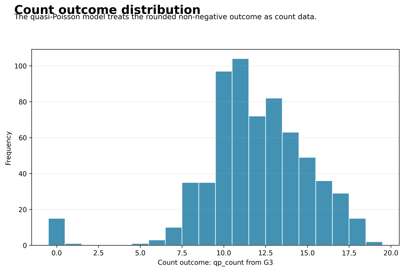
The outcome is restricted to the educational score range rather than having an unrestricted count tail. All 649 observations contribute to the distribution and the same values enter both the ordinary Poisson and scaled fits.
The bounded support provides a substantive reason why residual spread can be smaller than the Poisson mean benchmark. Confirm that treating G3 as a count-like outcome is scientifically defensible before using the narrower scaled intervals.
The chart matters because dispersion cannot be interpreted independently of measurement. Underdispersion is not an abstract software artifact here: the outcome cannot vary beyond its scoring limits. Review Histogram Interpretation when assessing concentration, tails and unusual score frequencies.
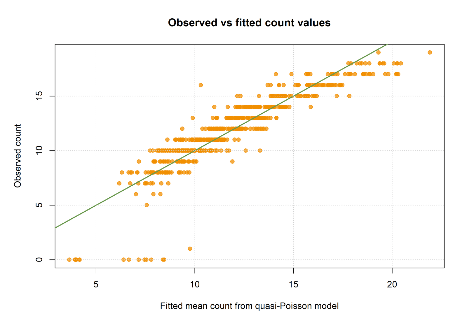
Python Chart 2: Observed Versus Fitted Counts
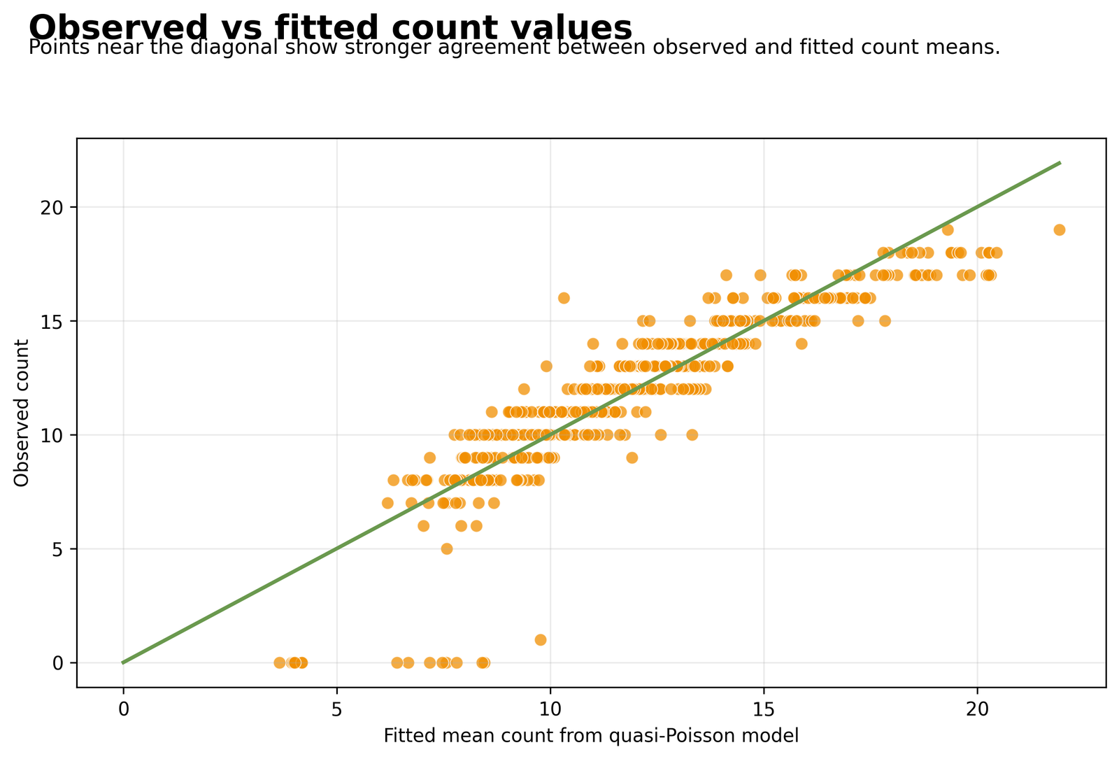
Standard Poisson fitted counts and Quasi Poisson Regression fitted counts coincide record by record. Example row 1 has an observed count of 11 and a fitted value of 11.508059 in both versions.
Any systematic departure from the diagonal concerns the conditional mean, not the scalar dispersion correction. Curvature, subgroup bias or range-specific errors would require formula revision rather than another change to φ.
This is the most direct visual proof that the analysis is a variance-only adjustment. Compare the calibration pattern with Residual Analysis before interpreting scaled significance decisions.
Python Chart 3: Pearson Residuals Versus Fitted Values
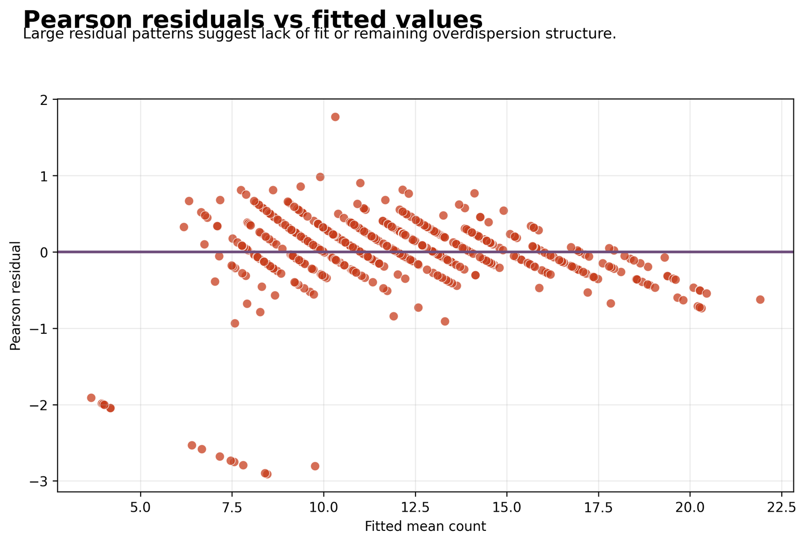
The squared Pearson residuals sum to 155.365855. Dividing by 639 residual degrees of freedom yields φ̂ = 0.243139, the defining numerical result of this Quasi Poisson Regression analysis.
A generally compressed cloud supports variance below the unit Poisson benchmark. A funnel, curve or subgroup band would warn that one global multiplier is not sufficient even when the average quotient is small.
The chart should be read with the fitted-value plot. A residual pattern can identify mean misspecification or changing spread that a single scale estimate hides. Diagnostic evidence is stronger when graphical and numerical checks agree.
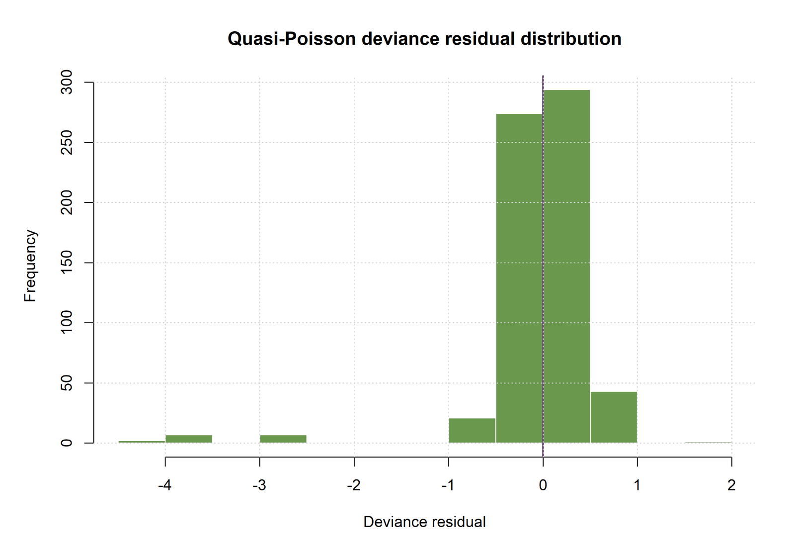
Python Chart 4: Deviance Residual Distribution
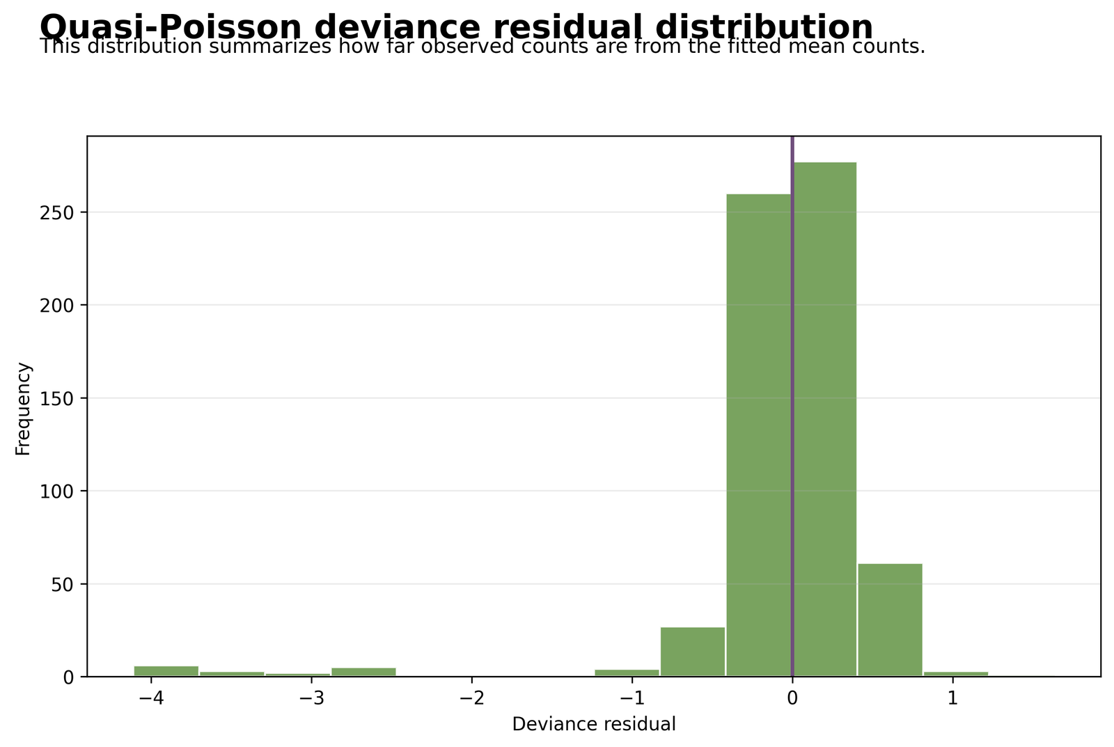
Residual deviance is 247.065469 in both model rows because the fitted means are unchanged. The distribution shows which observations make the largest contributions to lack of fit.
Asymmetry or extreme tails should trigger case review and mean-model checking. Deviance residuals remain useful diagnostics, but they do not create a complete quasi probability likelihood or a valid ordinary AIC.
Investigate unusual observations with Outlier Detection principles rather than deleting them automatically. A legitimate difficult case can reveal a missing predictor, interaction or measurement limitation.
Python Chart 5: Rate Ratios with Pearson-Scaled Intervals
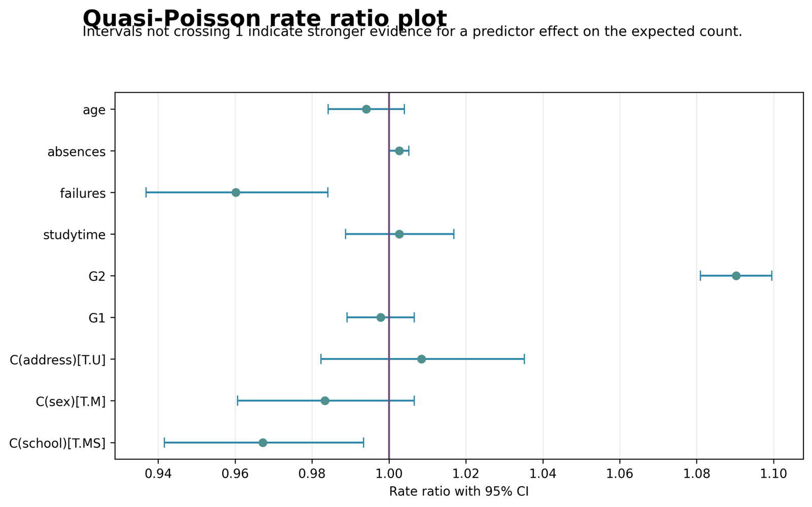
G2 is clearly above one at 1.090222 with a scaled 95% interval from 1.080959 to 1.099563. Failures is below one at 0.960220, while school MS is 0.967171 with interval 0.941624 to 0.993411.
Distance from one represents multiplicative magnitude; whether an interval crosses one represents statistical compatibility with no multiplicative effect. Terms near one can be statistically precise but practically small.
Every marker must be interpreted with its predictor unit and factor reference. Use Effect Size principles to keep magnitude separate from statistical significance.
Python Chart 6: Pearson Dispersion Check
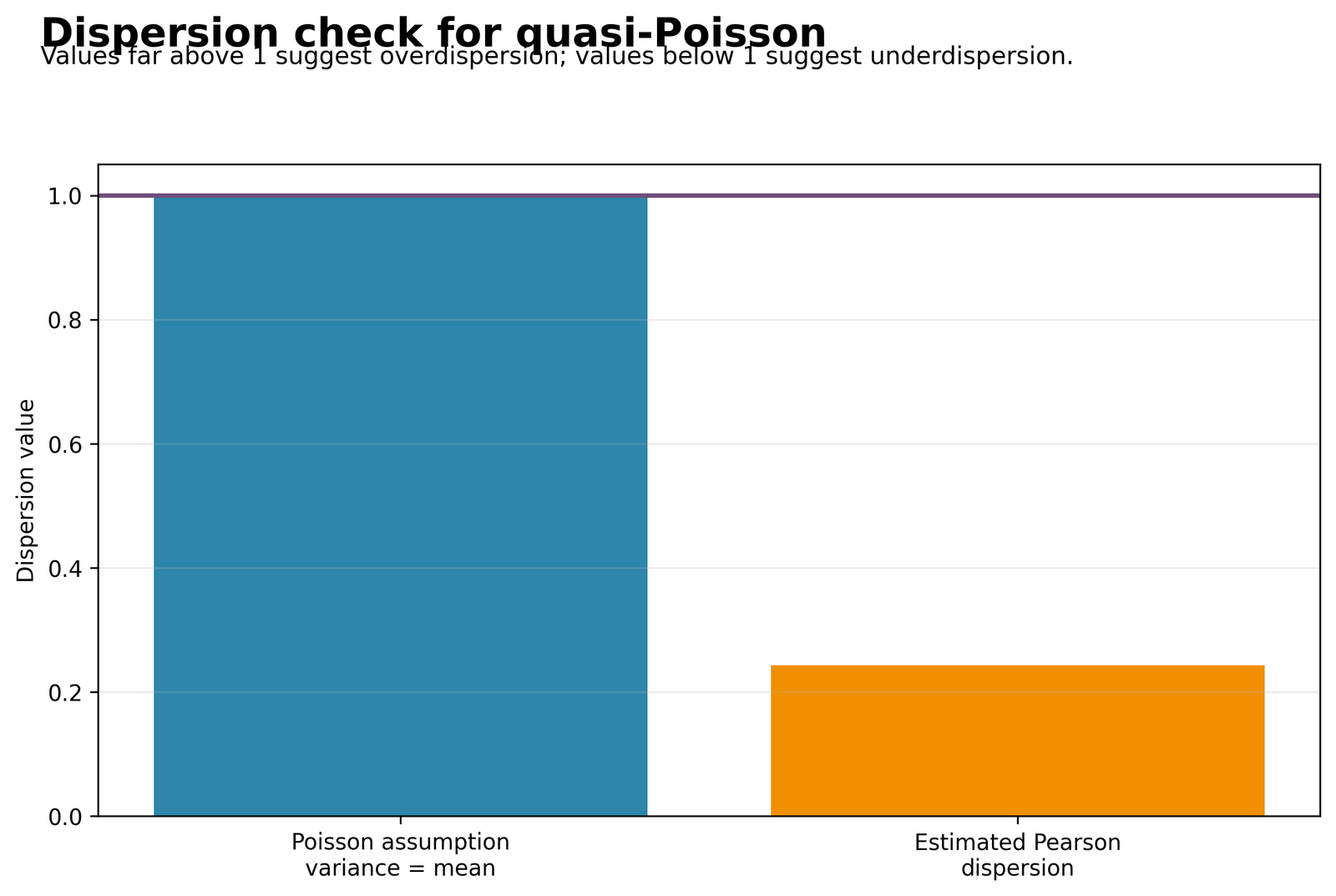
The estimated bar is near 0.243139, substantially below the benchmark value of one. The gap identifies strong underdispersion rather than the overdispersion more commonly used to introduce the method.
The scale justifies recalculating model-based covariance, but it does not prove that the outcome scale, independence assumption or mean specification is optimal. Verify those assumptions separately.
This chart is the visual summary of the article: the same fitted surface is accompanied by less residual variation than the ordinary Poisson covariance expects.
Python Chart 7: Observed and Fitted Counts Across G2
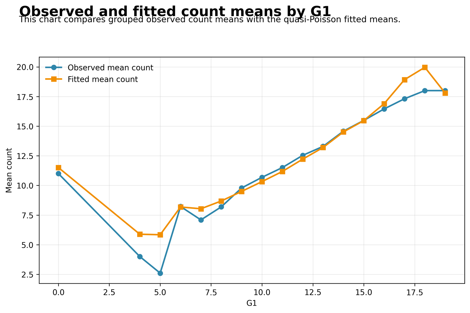
The fitted mean increases with G2, consistent with β = 0.086381 and rate ratio 1.090222 per one-point increase. Standard and quasi fitted lines overlap because φ does not modify β.
Check whether the observed pattern is approximately log-linear across the full G2 range. Systematic curvature would motivate a transformation, spline or interaction rather than a different scalar dispersion.
The chart connects the abstract rate ratio to the outcome scale. It also shows why a predictor-specific diagnostic is useful even when the global observed-versus-fitted plot appears acceptable.
R Quasi Poisson Regression Charts and Explanations
Quasi Poisson Regression in R provides an independent implementation of the same mean and Pearson-scaled uncertainty.
The R visuals provide one independent cross-software validation of the Python analysis. They use the same 649 observations, formula, factor references and log link. R reports dispersion of approximately 0.243141, closely matching the Python value 0.243139.
R chart pair 1: outcome distribution and fitted-mean calibration
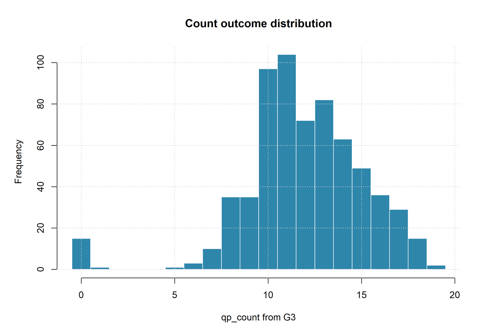
Bounded Count Distribution
The distribution confirms that the response is a bounded score treated as count-like. That restriction helps explain why the residual variance can be substantially below the Poisson mean benchmark.
The statistical meaning is not that every bounded response requires Quasi Poisson Regression. The chart supports the underdispersion story only when the log-linked conditional mean remains appropriate.
Observed Versus Fitted Counts
The points evaluate calibration of the shared conditional mean. The quasipoisson and poisson fitted values are identical to numerical precision because both solve the same mean equations.
Visible bias would indicate a mean-model problem. Changing the dispersion parameter cannot correct a missing nonlinear term, interaction, offset or predictor.
R chart pair 2: Pearson dispersion and deviance-residual evidence
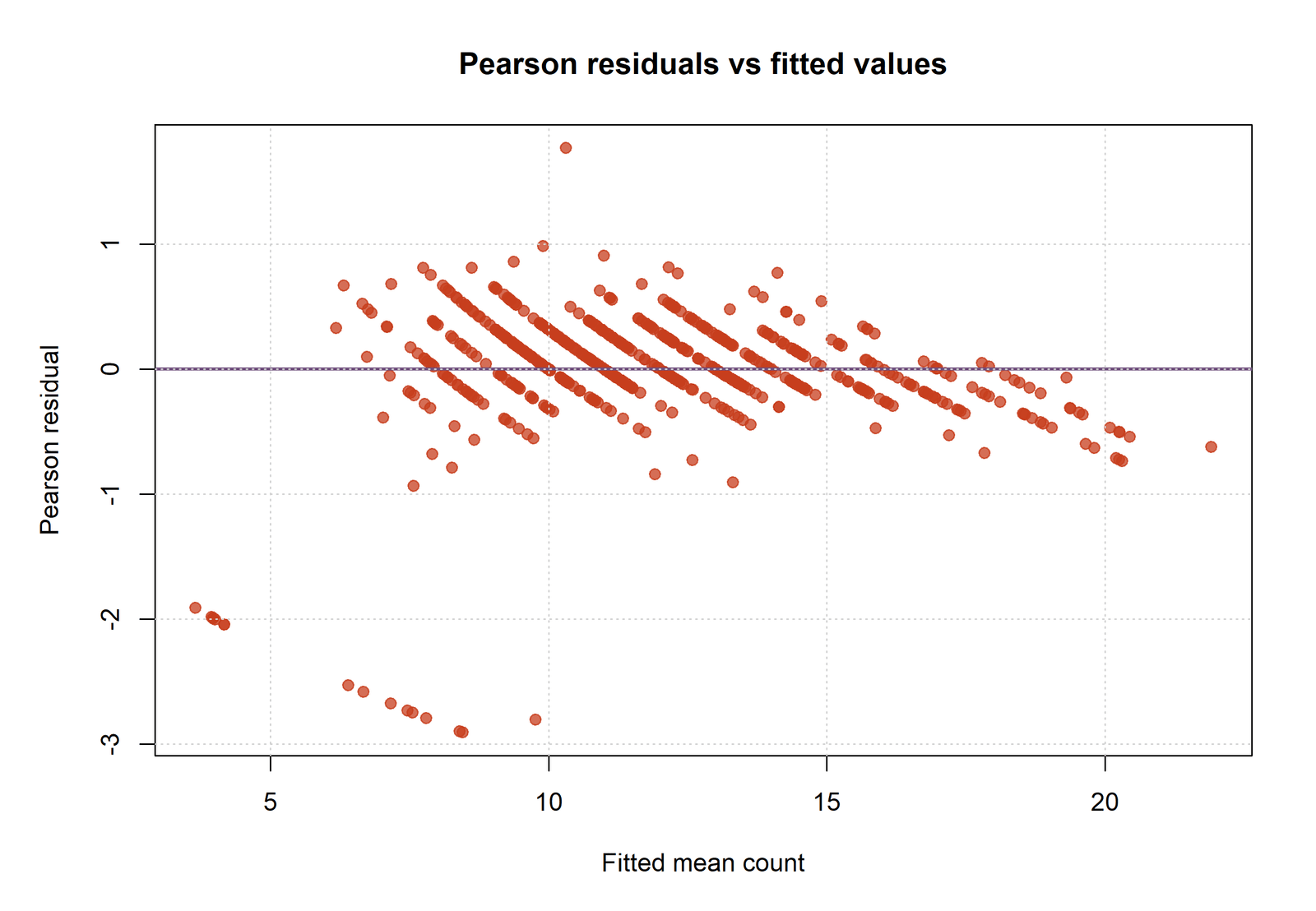
Pearson Residual Scale
The residual pattern supports the numerical scale estimate near 0.24314. Its overall contraction explains why the quasipoisson standard errors are smaller than the standard Poisson values.
A changing envelope would challenge the assumption that one φ applies across all fitted means. The global quotient should never be interpreted without its residual pattern.
Deviance Residual Distribution
The chart identifies records that contribute disproportionately to lack of fit while preserving the shared residual deviance of 247.065469. It complements, rather than replaces, Pearson residual analysis.
These residuals do not provide a full quasi likelihood. R’s NA AIC remains the correct model-output behavior.
Quasi Poisson Regression Coefficient Interpretation
Quasi Poisson Regression coefficients retain the same log-rate and rate-ratio interpretation used by the corresponding Poisson mean model.
Each coefficient is a change in the log conditional mean, and each exponentiated coefficient is a rate ratio. The term “rate ratio” is conventional even though this worked model has no exposure offset; technically, the ratio compares expected counts per observation under different predictor values.
G2: Main Positive Predictor
Holding G1, studytime, failures, absences, age, school, sex and address fixed, a one-point increase in G2 multiplies the fitted conditional mean by 1.090222. This is approximately a 9.02% increase because (1.090222 − 1) × 100 = 9.0222%. The scaled 95% interval, 1.080959 to 1.099563, remains entirely above one.
Failures: Negative Multiplicative Association
Each additional failure multiplies the adjusted fitted mean by 0.960220. The corresponding percentage change is about −3.978%. The Pearson-scaled interval is 0.936868 to 0.984155 and p = 0.001232. This is a conditional association and should not be interpreted causally.
Absences: Statistically Precise but Small Per-Unit Effect
Each additional absence multiplies the fitted mean by 1.002663, an increase of about 0.2663% per absence. The scaled interval is 1.000131 to 1.005202 and p = 0.039286. Because the per-unit effect is small, practical interpretation should consider meaningful multi-absence contrasts rather than focusing only on the threshold result.
School, Sex and Address Contrasts
MS versus GP has a rate ratio of 0.967171, M versus F has 0.983359, and U versus R has 1.008429. Only the school interval excludes one after Pearson scaling. These effects depend on the stated reference categories and adjustment set. Changing reference coding changes the displayed coefficient but not the underlying fitted comparison.
The intercept rate ratio 4.832001 describes the fitted mean when every numeric predictor equals zero and all factors are at their reference categories. Because age, G1 and G2 equal zero outside or near the edge of the substantive data region, the intercept is primarily a model anchor rather than a meaningful student profile.
Quasi Poisson Regression Predictions and Effects
Quasi Poisson Regression predictions in this analysis are identical to the standard Poisson fitted means because scalar dispersion does not alter beta.
Quasi Poisson Regression produces the same fitted conditional means as the companion Poisson model in this scalar-dispersion analysis. For row 1, the observed count is 11, the fitted count is 11.508059, the raw residual is −0.508059, the Pearson residual is −0.149766 and the deviance residual is −0.150889. Row 2 has observed 11 and fitted 11.291007; row 3 has observed 12 and fitted 13.636190.
| Row | Observed | Poisson fitted | Quasi fitted | Raw residual | Pearson residual | Deviance residual |
|---|---|---|---|---|---|---|
| 1 | 11 | 11.508059 | 11.508059 | −0.508059 | −0.149766 | −0.150889 |
| 2 | 11 | 11.291007 | 11.291007 | −0.291007 | −0.086604 | −0.086980 |
| 3 | 12 | 13.636190 | 13.636190 | −1.636190 | −0.443085 | −0.452421 |
| 4 | 14 | 14.606930 | 14.606930 | −0.606930 | −0.158803 | −0.159922 |
| 5 | 13 | 13.370057 | 13.370057 | −0.370057 | −0.101205 | −0.101677 |
A fitted mean is not a deterministic prediction of the next observed count. It is the conditional expectation under the specified covariate pattern. Confidence intervals for the mean can use the scaled coefficient covariance, but a probability prediction interval for a future observation requires additional distributional assumptions because the quasi model does not define a complete probability mass function.
For scenario analysis, construct the new design row using the same factor references and units, calculate η = x′β, and exponentiate to obtain μ̂. When comparing two profiles, exp(xA′β − xB′β) gives their fitted mean ratio. The result is meaningful only within the data-supported predictor range.
Quasi Poisson Regression Assumptions and Diagnostics
Quasi Poisson Regression diagnostics must evaluate both the shared log-linked mean and the proportional variance assumption.
Core Assumptions
- Nonnegative count-like response with a meaningful conditional mean.
- Correct log-linked functional form.
- Variance approximately proportional to μ through one φ.
- Independent observations for the displayed model-based covariance.
- Correct factor coding, offsets, weights and retained rows.
- Adequate information for large-sample Wald inference.
Required Diagnostic Questions
- Do observed and fitted values show systematic bias?
- Are Pearson residuals centered without a changing envelope?
- Do deviance residuals reveal extreme or asymmetric cases?
- Does one φ summarize spread across predictor ranges and groups?
- Are G1 and G2 coefficients stable under collinearity checks?
- Would clustering, zero inflation or another outcome scale matter?
Mean-Model Adequacy
Residual scaling cannot correct a missing predictor, nonlinear relationship or interaction. Examine residuals against fitted values and important predictors. A curve around zero indicates a functional-form problem. A subgroup shift indicates an omitted interaction or level effect. Review the broader Regression Assumptions and Regression Diagnostics workflows.
Variance Proportionality
The single-scale model assumes Var(Y|X)/μ is approximately constant. A funnel or group-specific spread can make the average φ̂ misleading. In that situation, consider robust covariance, an alternative variance function, group-specific modeling or a different count distribution.
Independence and Clustering
Students may share school-level conditions, but the worked covariance treats observations as independent. Including school as a fixed predictor adjusts the mean contrast; it does not model within-school correlation. Dependence should be addressed with a design-specific method.
Collinearity and Predictor Stability
G1 and G2 measure related academic history. Use Variance Inflation Factor and Tolerance Statistic to assess coefficient stability. A variance-scale correction does not alter the design matrix or solve collinearity.
Influential Observations
Large residuals and high-leverage profiles can affect the mean coefficients and therefore every fitted count. Use Cook’s Distance and Influence Diagnostics with generalized-linear-model adaptations. Investigate data quality and substantive legitimacy before changing the analysis sample.
The essential validation pattern is present: coefficients and fitted means match across the standard and scaled rows; Pearson chi-square and residual degrees of freedom reproduce φ̂; Python and R scales agree closely; and R correctly leaves AIC unavailable.
Quasi Poisson Regression in SPSS, Python, R and Excel
Quasi Poisson Regression software output is comparable only when every implementation uses the same sample, formula, references, link and scale estimator.
Python
Fit the Poisson mean with a log link, obtain Pearson chi-square and residual degrees of freedom, calculate φ̂, and rescale the normalized covariance. Keep paired standard and scaled tables so unchanged coefficients can be audited.
- Best for transparent covariance calculations
- Verify fitted-value equality
- Do not label a scaled Poisson likelihood field as quasi AIC
R
Use glm(..., family = quasipoisson(link = "log")). The summary reports the estimated dispersion, and AIC() returns NA because no ordinary quasi likelihood is available.
- Direct quasipoisson family
- Convenient coefficient and diagnostic workflow
- Useful independent validation of Python
SPSS
Use GENLIN with Poisson distribution, log link and Pearson scale estimation. Confirm the categorical references and whether the output uses fixed or estimated scale before reading the parameter tests.
- Menu-driven and syntax-based analysis
- Check scale setting explicitly
- Export parameter and fit tables together
Excel
Use the workbook to reproduce φ̂, √φ̂, scaled standard errors, z values, p-values and exponentiated confidence limits. Excel is valuable for arithmetic verification but is not the primary fitting engine for this worked model.
- Clear formula audit trail
- Useful for teaching and reporting
- Keep full precision in calculation cells
Software should agree only after the same rows, formula, factor references, link, offset, scale estimator and confidence method are used. The article performs the cross-software check once here rather than repeating it after every chart.
Quasi Poisson Regression Code
Quasi Poisson Regression code should preserve the mean fit, expose the dispersion calculation and label scaled inference accurately.
Expand only the software workflow needed for the analysis. Replace the illustrative file-loading line with the local dataset path while retaining the same variable names and factor references.
Python: fit the shared mean and calculate Pearson scaling
import numpy as np
import pandas as pd
import statsmodels.api as sm
import statsmodels.formula.api as smf
from scipy.stats import norm

df = pd.read_csv("dataset.csv")
df["count_outcome"] = df["G3"].round().clip(lower=0).astype(int)

formula = (
    "count_outcome ~ G1 + G2 + studytime + failures + "
    "absences + age + C(school) + C(sex) + C(address)"
)

poisson = smf.glm(
    formula=formula,
    data=df,
    family=sm.families.Poisson(link=sm.families.links.Log())
).fit()

phi = poisson.pearson_chi2 / poisson.df_resid
scaled_cov = phi * poisson.normalized_cov_params
scaled_se = np.sqrt(np.diag(scaled_cov))
scaled_z = poisson.params.to_numpy() / scaled_se
scaled_p = 2 * norm.sf(np.abs(scaled_z))

lower_beta = poisson.params.to_numpy() - 1.96 * scaled_se
upper_beta = poisson.params.to_numpy() + 1.96 * scaled_se

result = pd.DataFrame({
    "beta": poisson.params,
    "scaled_se": scaled_se,
    "z": scaled_z,
    "p": scaled_p,
    "rate_ratio": np.exp(poisson.params),
    "rr_lower": np.exp(lower_beta),
    "rr_upper": np.exp(upper_beta)
})

print("Pearson chi-square:", poisson.pearson_chi2)
print("Residual df:", poisson.df_resid)
print("Dispersion:", phi)
print(result)
R: fit quasipoisson and report scaled rate ratios
dat <- read.csv("dataset.csv", stringsAsFactors = FALSE)
dat$count_outcome <- as.integer(pmax(round(dat$G3), 0))

dat$school  <- relevel(factor(dat$school), ref = "GP")
dat$sex     <- relevel(factor(dat$sex), ref = "F")
dat$address <- relevel(factor(dat$address), ref = "R")

fit_q <- glm(
  count_outcome ~ G1 + G2 + studytime + failures +
    absences + age + school + sex + address,
  family = quasipoisson(link = "log"),
  data = dat
)

summary(fit_q)
summary(fit_q)$dispersion

coef_table <- summary(fit_q)$coefficients
rr <- exp(coef(fit_q))
rr_ci <- exp(confint.default(fit_q))

cbind(coef_table, rate_ratio = rr, rr_ci)
AIC(fit_q)  # NA for a true quasi-likelihood fit
SPSS: GENLIN with Pearson scale estimation
GENLIN count_outcome BY school sex address
  WITH G1 G2 studytime failures absences age
  /MODEL school sex address G1 G2 studytime failures absences age
    INTERCEPT=YES
    DISTRIBUTION=POISSON
    LINK=LOG
  /CRITERIA SCALE=PEARSON CILEVEL=95
  /PRINT CPS DESCRIPTIVES MODELINFO FIT SUMMARY SOLUTION.
Confirm the factor reference categories in the SPSS output. The desired comparisons are MS versus GP, M versus F, and U versus R.
Excel: reproduce the dispersion and scaled interval arithmetic
Pearson dispersion:
=155.365855/639

Square-root scale:
=SQRT(155.365855/639)

Scaled standard error:
=Poisson_SE*SQRT($B$2)

Scaled z statistic:
=Beta/Scaled_SE

Two-sided normal p-value:
=2*(1-NORM.S.DIST(ABS(Scaled_z),TRUE))

Lower rate-ratio limit:
=EXP(Beta-1.96*Scaled_SE)

Upper rate-ratio limit:
=EXP(Beta+1.96*Scaled_SE)
Keep the unrounded φ value in the calculation cell and apply formatting only to displayed results.
Advanced Quasi Poisson Regression Topics
These 26 expandable panels address the issues that most often determine whether Quasi Poisson Regression is scientifically appropriate, correctly implemented and accurately reported.
1. Mean Model and Variance Model Are Different Decisions
Quasi Poisson Regression preserves the log-linked conditional mean while replacing the fixed Poisson variance with φμ. This separation matters because a satisfactory mean equation can coexist with an inadequate variance assumption. In the worked analysis, every coefficient and fitted count matches the companion Poisson model, yet the estimated covariance is much smaller because φ̂ = 0.243139.
A report should therefore identify which layer changed. Saying that Quasi Poisson Regression “found a different effect” would be incorrect here. The fitted association is the same; the estimated precision is different.
2. Why Scalar Dispersion Leaves Coefficients Unchanged
With a constant dispersion multiplier, the scalar appears in every observation’s variance contribution and cancels from the estimating equation for β. The solution for β is therefore the same as under the corresponding Poisson mean model. Quasi Poisson Regression changes the covariance matrix after the mean coefficients have been estimated.
This property is an important implementation check. Standard and scaled rows should have identical β values and identical rate ratios. Materially different point estimates would mean that the formulas, data, link, weights, offset, or missing-data rules were not actually held constant.
3. Underdispersion Is a Valid Quasi Result
Many introductions emphasize overdispersion because it is common in event counts, but Quasi Poisson Regression also permits φ below one. The present estimate of 0.243139 indicates that the observed Pearson variation is only about one quarter of the unit-dispersion benchmark after accounting for the model degrees of freedom.
The bounded 0–20 grade scale makes underdispersion plausible because the response cannot develop the unrestricted right tail of a conventional count process. The direction must be reported from the data rather than changed to match a familiar textbook example.
4. Bounded Counts and Measurement Choice
The response was created from G3 and treated as a nonnegative count-like variable. Although the log-link calculation is valid for that engineered outcome, G3 is also a bounded educational score. Quasi Poisson Regression answers a conditional-mean question on the multiplicative count scale; it does not prove that this is the only or best measurement representation.
Researchers should compare the substantive meaning of a count model with continuous, ordinal, or bounded-outcome alternatives. The most defensible model is the one whose outcome scale, assumptions, and interpretation align with the research question.
5. Pearson Dispersion Versus Deviance Dispersion
The worked Quasi Poisson Regression analysis uses Pearson chi-square divided by residual degrees of freedom: 155.365855 / 639 = 0.243139. A deviance-based quotient would use a different numerator and can produce a different scale estimate. The report must identify which estimator generated the displayed standard errors.
Pearson scaling is especially transparent because the same residuals appear in the diagnostic plot. Mixing a Pearson scale in one table with deviance-scaled intervals in another would make the results internally inconsistent.
6. Degrees of Freedom in the Scale Estimate
The denominator is 639 rather than 649 because ten regression parameters were estimated: the intercept, six numeric predictors, and three factor contrasts. Using the sample size alone would underestimate the scale adjustment slightly and propagate the error into every standard error and confidence interval.
Quasi Poisson Regression software usually handles the residual degrees of freedom automatically, but a worked calculation should still display the numerator, denominator, and quotient. That audit trail makes the scale reproducible.
7. Rate Ratios and Predictor Units
Exponentiating a coefficient gives a multiplicative change in the conditional mean for a one-unit predictor increase, holding the other terms fixed. For G2, exp(0.086381) = 1.090222, so the fitted mean is multiplied by about 1.090 for each one-point increase in G2.
The practical interpretation depends on the unit. A one-point grade increase differs from a one-year age increase or a one-absence increase. Quasi Poisson Regression does not standardize those units automatically, so every reported rate ratio must retain its original scale.
8. Factor References and Contrast Interpretation
The factor contrasts compare MS with GP for school, M with F for sex, and U with R for address. The school rate ratio of 0.967171 describes the adjusted MS-to-GP multiplicative contrast under those reference settings. Reversing the reference category would invert the rate ratio.
Reference coding must be reported beside the coefficient table because the sign alone is not self-explanatory. Quasi Poisson Regression scaling changes uncertainty but does not change the contrast definition.
9. Statistical Significance After Underdispersion Scaling
When φ̂ is below one, standard errors contract by approximately √φ̂. Here √0.243139 is about 0.493, so many scaled standard errors are roughly half their unscaled values. That is why the school, failures, and absences terms cross conventional significance thresholds in the scaled table.
The change should be described as a covariance decision, not as a new coefficient. A small p-value still requires effect-size interpretation, design evaluation, and consideration of whether the proportional-variance assumption is credible.
10. Why Ordinary AIC Is Unavailable
Ordinary AIC is built from a maximized probability likelihood. Quasi Poisson Regression specifies a mean and variance relationship without defining a complete probability mass function, so a standard likelihood-based AIC is not available. R appropriately returns NA for the quasipoisson fit.
The numeric field produced by treating a scaled Poisson object as though it were a quasi likelihood should not be used for model ranking. Model comparison should instead use diagnostic adequacy, predictive evaluation, cross-validation, or methods designed for quasi-likelihood settings.
11. QAIC Requires Explicit Conventions
Some disciplines use quasi-AIC variants, often called QAIC, but the calculation depends on a specified likelihood surrogate, an estimated overdispersion parameter, and a clearly stated parameter count. Those conventions are not interchangeable with ordinary AIC.
Because this worked analysis documents underdispersion and does not define a QAIC protocol, the safest report leaves ordinary AIC unavailable. A custom QAIC should never appear without its exact formula and justification.
12. Robust Covariance Is Not the Same Model
A sandwich or heteroskedasticity-robust covariance can protect inference against a broader class of variance misspecification. Quasi Poisson Regression instead imposes the proportional relationship Var(Y|X) = φμ. The two approaches can produce different standard errors even when they share the same mean coefficients.
Choosing between them depends on the scientific variance assumption, independence structure, and sample properties. Robust covariance does not create a negative-binomial probability model, and quasi scaling does not automatically provide cluster-robust inference.
13. Clustered Observations Need More Than One Phi
If students within the same school are correlated, a single dispersion parameter cannot represent that dependence. The present model includes school as a fixed contrast but does not model within-school residual correlation. Quasi Poisson Regression therefore addresses marginal variance scaling, not hierarchical dependence.
For genuine clustering, compare Generalized Estimating Equations, Multilevel Regression, or cluster-robust covariance methods. The estimand and correlation structure should guide the choice.
14. Exposure Offsets and Rate Interpretation
Count models often include log exposure as an offset so coefficients describe rates per unit of time, population, or opportunity. No offset appears in this worked equation, so the fitted quantity is an expected grade count per observation rather than an event rate standardized by exposure.
Adding an offset would change the mean specification and therefore the fitted values. It would no longer be a pure covariance-only comparison with the present Quasi Poisson Regression results.
15. Nonlinearity in the Log Mean
Quasi scaling cannot repair an incorrect functional form. If the relationship between G2 and log(μ) is curved, the residual pattern can remain systematic even after the dispersion estimate is correct on average. Splines, transformations, or interactions may be needed.
Residuals versus fitted values and predictor-specific plots should therefore be reviewed before relying on the scaled tests. A good variance adjustment does not substitute for a well-specified conditional mean.
16. Interactions and Conditional Rate Ratios
An interaction makes a rate ratio conditional on another predictor. For example, a G2-by-school interaction would allow the G2 multiplicative slope to differ between GP and MS. The present Quasi Poisson Regression model contains only main effects, so its rate ratios assume a common slope across factor levels.
Interactions should be added for a substantive reason and interpreted using predicted means or combined coefficients. Reporting only the component p-values can obscure the conditional effect.
17. Zero Inflation Is a Separate Mean-Distribution Issue
An excess number of zeros can indicate a mixture process in which some observations are structurally unable to produce a positive count. Quasi Poisson Regression adjusts the variance around one mean process; it does not create a separate zero-generating component.
When zeros dominate the data, compare a Zero-Inflated Poisson Regression or Hurdle Regression model. In this grade example, the bounded scale is more central than a structural-zero mechanism.
18. Negative Binomial Regression Has a Different Variance Shape
Negative Binomial Regression typically uses a variance that grows faster than the mean, often μ + αμ². It is a full likelihood model designed mainly for overdispersion. The present φ̂ below one does not match that conventional variance direction.
Quasi Poisson Regression is therefore not merely a less sophisticated negative-binomial model. It answers a different variance question and can represent both overdispersion and underdispersion through a scalar multiplier.
19. Prediction Intervals Need a Full Distribution
Confidence intervals for the expected mean can be built from the scaled coefficient covariance. A probability prediction interval for a future count is more difficult because Quasi Poisson Regression does not specify a complete sampling distribution.
Reports should distinguish uncertainty in the fitted mean from uncertainty in a new observation. A narrow coefficient interval does not imply that exact future outcomes can be predicted with the same narrowness.
20. Influence and Case-Level Sensitivity
Large Pearson or deviance residuals identify observations that the mean equation fits poorly. Case-deletion influence can also be assessed by refitting or by generalized linear-model diagnostics. Quasi scaling changes the covariance scale but does not erase influential observations.
Use Outlier Detection and Influence Diagnostics as complements. Cases should be investigated for data quality and substantive legitimacy before any exclusion decision.
21. Cross-Software Agreement and Small Numerical Differences
Python reports φ̂ = 0.243139 and R reports approximately 0.243141. Such tiny differences can arise from printed precision, implementation details, and the exact object used for covariance extraction. They do not represent a substantive disagreement.
Cross-software validation should compare the formula, reference levels, rows retained, fitted means, coefficients, degrees of freedom, and scale estimator. Matching labels alone is not enough.
22. Small-Sample and Sparse-Design Concerns
Wald tests rely on large-sample approximations. Although n = 649 is substantial, sparse factor combinations or highly correlated predictors can still make individual terms unstable. The number of observations should not be treated as the only measure of information.
Quasi Poisson Regression reports should examine cell counts, coefficient correlations, and sensitivity to specification. Small-sample corrections may be necessary in designs with few independent clusters even when the row count is large.
23. Collinearity Between G1 and G2
G1 and G2 are related prior-grade measures. Their joint inclusion makes each coefficient a partial effect holding the other grade fixed, which differs from its unadjusted association with G3. A small G1 coefficient does not mean G1 is unrelated to the outcome overall.
Review Variance Inflation Factor and Tolerance Statistic when interpreting correlated predictors. Dispersion scaling does not solve collinearity.
24. Causal Language Remains Unsupported
Quasi Poisson Regression estimates conditional associations under the specified observational design. It does not create random assignment, remove omitted-variable bias, or establish temporal ordering. A precise rate ratio can still be noncausal.
Use wording such as “was associated with” or “the fitted mean differed by” unless the study design supports stronger claims. The variance correction changes precision, not identification.
25. Reproducible Reporting and Rounding
Calculations should retain full precision while tables use consistent rounding. For example, φ̂ can be reported as 0.2431 while the reproducibility line retains 155.365855 / 639. Rate ratios and confidence limits should be rounded together so the interval remains coherent.
Downloadable code, tables, and the worked workbook allow readers to verify the analysis without crowding the public article with 649 repetitive rows. This is more useful than publishing an oversized raw ledger in the post body.
26. Choosing the Final Model
The final choice should follow the outcome’s scientific scale, the mean pattern, the variance pattern, the dependence structure, and the intended estimand. Quasi Poisson Regression is attractive when the log mean is suitable and a proportional scale adjustment captures residual variation.
It is less suitable when a full probability likelihood is required, zero processes must be modeled separately, exposure rates are central but omitted, clustering is unaddressed, or the bounded grade should be analyzed on another scale. Model selection is therefore a reasoned decision, not a contest for the smallest p-value.
APA-Style Quasi Poisson Regression Reporting
A complete report identifies the outcome construction, log link, predictor set, factor references, variance function, dispersion estimator and the inferential scale used for coefficients. It should also explain that ordinary likelihood-based AIC is unavailable.
Worked APA-style result: A Quasi Poisson Regression with a log link was fitted to the G3-derived count for 649 students using G1, G2, studytime, failures, absences, age, school, sex and address as predictors. Pearson chi-square was 155.366 on 639 residual degrees of freedom, yielding φ̂ = 0.2431 and indicating underdispersion. Pearson scaling left the regression coefficients, rate ratios and fitted means unchanged but reduced the model-based standard errors. G2 was positively associated with the fitted conditional mean, β = 0.0864, SE = 0.0044, rate ratio = 1.0902, 95% CI [1.0810, 1.0996], p < .001. Failures was negatively associated with the fitted mean, β = −0.0406, SE = 0.0126, rate ratio = 0.9602, 95% CI [0.9369, 0.9842], p = .001. Ordinary likelihood-based AIC was not reported because the quasi model does not define a complete probability likelihood.
When a standard Poisson comparison is included, label it as an inferential sensitivity analysis. Do not place an unscaled p-value beside a scaled confidence interval. Report exact p-values when practical, use p < .001 for extremely small values, and retain enough digits for rate ratios close to one.
Quasi Poisson Regression Publication Checklist
Model and Data
- Define why the response is count-like.
- State the sample size and missing-data rule.
- List numeric predictors and factor references.
- State whether an offset, weight or interaction was used.
- Show the log-linked mean and φμ variance function.
- Explain why Quasi Poisson Regression was selected.
Results and Diagnostics
- Report Pearson chi-square, residual df and φ̂.
- Confirm coefficients and fitted means match Poisson.
- Use scaled SEs, intervals and p-values consistently.
- Do not report ordinary quasi AIC.
- Review residual, influence and dependence diagnostics.
- Separate statistical precision from practical magnitude.
Final quality check: the headline, Quick Answer, tables, charts, code, APA paragraph and conclusion must all describe the same underdispersed Quasi Poisson Regression result. No section should call φ̂ = 0.243139 overdispersion.
Quasi Poisson Regression Downloads
R Quasi Poisson Regression ReportIndependent quasipoisson fit, dispersion estimate, coefficient table and chart verification.
SPSS Quasi Poisson Regression OutputGENLIN scale-estimation output and parameter results.
Worked Quasi Poisson Regression Excel WorkbookPearson dispersion, scaled standard errors, tests, confidence intervals and fitted-value audit.
Quasi Poisson Regression Frequently Asked Questions
1. What is Quasi Poisson Regression?
Quasi Poisson Regression is a generalized linear modeling approach that uses the Poisson log-linked mean but estimates a dispersion parameter so the conditional variance is φ times the mean.
2. When should Quasi Poisson Regression be used?
Use Quasi Poisson Regression when the response is nonnegative and count-like, the log-linked mean is scientifically reasonable, and the observed variance is not well represented by the fixed Poisson equality Var(Y|X)=μ.
3. Does Quasi Poisson Regression require overdispersion?
No. It can estimate φ above one for overdispersion or below one for underdispersion. The worked result φ̂=0.243139 indicates underdispersion.
4. Why are the fitted values identical to Poisson?
A constant dispersion multiplier cancels from the coefficient estimating equations. With the same data, formula, link, weights, and offset, the Quasi Poisson Regression coefficients and fitted means match the Poisson model.
5. What changes after Pearson scaling?
The covariance matrix, standard errors, test statistics, p-values, and confidence intervals change. The coefficients, rate ratios, linear predictor, and fitted means do not change.
6. How is the dispersion parameter calculated?
This analysis divides Pearson chi-square by residual degrees of freedom: 155.365855 / 639 = 0.243139.
7. What does φ below one mean?
It means the residual variation is smaller than the ordinary Poisson variance benchmark after adjustment for the fitted mean and model degrees of freedom.
8. Can ordinary AIC be reported for Quasi Poisson Regression?
No ordinary likelihood-based AIC should be reported because the quasi model does not define a complete probability likelihood. R correctly returns NA for this fit.
9. How is a rate ratio interpreted?
Exponentiate the coefficient. For G2, exp(0.086381)=1.090222, so each one-point increase in G2 multiplies the adjusted conditional mean by about 1.090, holding the other predictors fixed.
10. Why did the school result become significant?
The school coefficient and rate ratio did not change. Because φ̂ was below one, its standard error decreased from 0.027699 to 0.013658, producing p=0.014525 and a scaled rate-ratio interval of 0.941624 to 0.993411.
11. Is a smaller p-value automatically better?
No. It is only appropriate when the proportional-variance and independence assumptions are defensible. Statistical precision must be interpreted with effect magnitude, study design, and model adequacy.
12. Does Quasi Poisson Regression handle repeated or clustered data?
Not by itself. A scalar φ does not model correlation among observations. Use GEE, cluster-robust covariance, or a multilevel count model when dependence is part of the design.
13. Is Quasi Poisson Regression the same as Negative Binomial Regression?
No. Negative binomial regression defines a full probability model with a variance that usually grows quadratically with the mean. Quasi Poisson Regression uses a proportional variance φμ and does not provide an ordinary likelihood AIC.
14. Can Quasi Poisson Regression produce prediction intervals?
It can support intervals for the expected mean through the scaled coefficient covariance, but a full probability prediction interval for a future count requires additional distributional assumptions.
15. Which software result should be reported?
Report the result from the implementation whose formula, factor references, scale estimator, and retained observations match the analysis plan. Python and R should be used as a single cross-software validation, not mixed term by term.
16. What is the main conclusion of this worked analysis?
The fitted mean model is unchanged, but Pearson scaling indicates strong underdispersion. The final report should state φ̂=0.243139, unchanged rate ratios and fitted counts, narrower scaled uncertainty, and the absence of ordinary quasi-likelihood AIC.
Quasi Poisson Regression Conclusion
This worked Quasi Poisson Regression analysis demonstrates a clean separation between the conditional mean and its uncertainty. The log-linked mean, regression coefficients, rate ratios and fitted counts are identical to the companion Poisson model. Pearson chi-square of 155.365855 on 639 residual degrees of freedom produces φ̂ = 0.243139, identifying strong underdispersion and reducing model-based standard errors by a factor of about 0.493.
G2 remains the principal positive predictor with rate ratio 1.090222. Failures has rate ratio 0.960220, and the school MS-to-GP contrast has rate ratio 0.967171. Their scaled intervals and tests are more precise, but the underlying associations have not changed. Absences illustrates why statistical precision should not be confused with practical magnitude.
The defensible conclusion is therefore specific: Quasi Poisson Regression retains the fitted Poisson mean while replacing unit-dispersion covariance with a Pearson-scaled covariance appropriate to the observed underdispersion. The result is useful only if the bounded count-like outcome, log mean, proportional variance and independence assumptions are acceptable. Ordinary quasi AIC must remain unavailable, and clustering, zero processes or alternative measurement scales require separate modeling decisions.
For the closest methodological comparisons, continue with Poisson Regression, Negative Binomial Regression and Generalized Estimating Equations.

