
Hurdle Model: Formula, Interpretation, SPSS, Python, R and Excel Guide
A Hurdle Model separates the question “Is the count zero or positive?” from the question “How large is the count after it becomes positive?” This worked analysis uses 649 observations, explains both components, and interprets every diagnostic chart before moving to software and advanced methods.
405 positive counts
8 Python + 8 R charts
SPSS · Python · R · Excel
Model Overview
What this model is and when it is used: A Hurdle Model is a two-part regression model for a non-negative count outcome that contains many zeros and a separate distribution of positive values. It is used when the process that determines whether an observation is zero is meaningfully different from the process that determines how large the count becomes after it is positive, such as no hospital visits versus the number of visits among patients who attended, no purchases versus purchase frequency, or no absences versus the number of absences. The dependent variable must be a count coded 0, 1, 2, 3 and so on, while the predictors may be continuous, ordinal, binary or categorical variables; categorical predictors are represented through reference-coded indicator variables. The first component usually uses logistic regression for zero versus positive, and the second uses a zero-truncated Poisson or negative-binomial count model for positive observations only.
Quick Answer
Part 1 — Crossing the hurdle
The binary model predicts whether hurdle_count > 0.
- school_MS: OR = 0.5339, p = .0017
- G1: OR = 0.7846, p = .0003
- G3: OR = 1.3058, p = .0003
Part 2 — Positive-count magnitude
The count model predicts the expected count among the 405 positive cases.
- school_MS: RR = 0.6528, p < .001
- G3: RR = 0.9313, p = .0034
- studytime: RR = 0.9029, p = .0002
- age: RR = 1.1108, p < .001
Table of Contents
- Why this dataset needs a Hurdle Model
- How the two-part model works
- Variables used
- Results at a glance
- Eight chart stories
- R charts with matching explanation boxes
- Complete coefficient tables
- Combined predictions
- Diagnostics and model choice
- SPSS, Python, R and Excel
- Code
- Advanced interpretation
- APA-style reporting
- Publication checklist
- Downloads
- Related guides
- FAQs
Why This Dataset Needs a Hurdle Model
A standard Poisson regression assumes one count-generating process and equidispersion. The worked outcome violates that simple picture in two ways: a large zero group and a positive tail whose variance greatly exceeds its mean.
The Hurdle Model treats zero as a decision boundary. One model estimates the chance of moving above zero. A separate zero-truncated count model estimates the size of the outcome among observations that have already crossed the boundary.
How the Two-Part Hurdle Model Works
Predict P(Y > 0) with a logit model.
Predict E(Y | Y > 0) with a zero-truncated count model.
Multiply the two predictions on the original count scale.
The first component produces log-odds coefficients and odds ratios. The second produces log-rate coefficients and rate ratios. Because the two components represent different mechanisms, the same predictor may increase one component and decrease the other.
For example, G3 raises the probability of a positive count but reduces the expected magnitude among positive observations. Its total effect on the unconditional expected count therefore depends on the full covariate profile.
Variables Used and Coding
| Variable | Role | Definition | Model use |
|---|---|---|---|
| hurdle_count | Outcome | MAX(0, ROUND(absences, 0)) | Non-negative count from 0 to 32 |
| hurdle_positive | Binary outcome | 1 when hurdle_count > 0; otherwise 0 | Crossing the hurdle |
| G1 | Predictor | First-period grade | Included in both components |
| G2 | Predictor | Second-period grade | Included in both components |
| G3 | Predictor | Final grade | Included in both components |
| studytime | Predictor | Study-time category | Included in both components |
| failures | Predictor | Previous class failures | Included in both components |
| age | Predictor | Age in years | Included in both components |
| Medu | Predictor | Mother’s education | Included in both components |
| school | Categorical predictor | MS compared with GP | GP is the reference |
| sex | Categorical predictor | M compared with F | F is the reference |
| address | Categorical predictor | U compared with R | R is the reference |
Results at a Glance
AIC = 834.4525
Null deviance = 859.345
AIC = 2444.9760
Substantial overdispersion
p < .001; Nagelkerke R² = .101
p < .001; Pearson/df = 3.000
Download the PDF Outputs
The same reports are available again in the complete Downloads section near the end of the post.
Eight Chart Stories: What Each Figure Actually Means
Each figure is interpreted in four steps: what it shows, exact values, statistical meaning and the next diagnostic action. This keeps the charts central to the analysis rather than treating them as decoration.
Chart 1: The Count Distribution and the Zero Spike
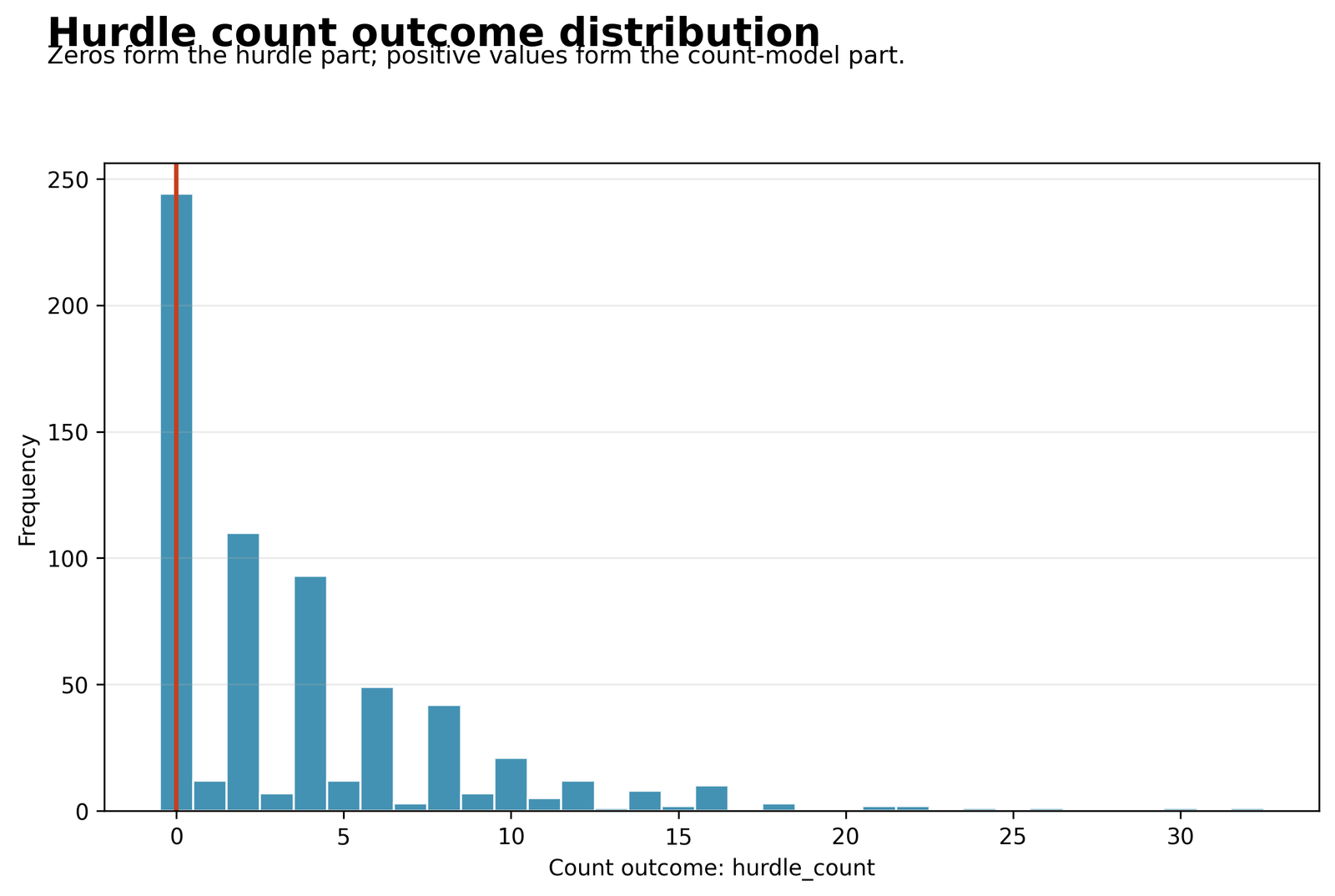
This histogram answers the first model-selection question: can one ordinary count distribution plausibly represent both the zero mass and the positive tail?
244 zeros and 405 positive counts are observed. The overall mean is 3.6595. Among positive cases, mean = 5.8642, median = 4, SD = 4.646, variance = 21.583, skewness = 1.995, kurtosis = 5.619, and range = 1–32.
The positive-count variance is about 3.68 times its mean, and the distribution has a heavy right tail. A simple equidispersed Poisson model is therefore too restrictive for the positive process.
Use a dedicated binary hurdle component for zero versus positive and compare the positive Poisson component with a zero-truncated negative-binomial alternative.
Chart 2: Zero Counts Versus Positive Counts
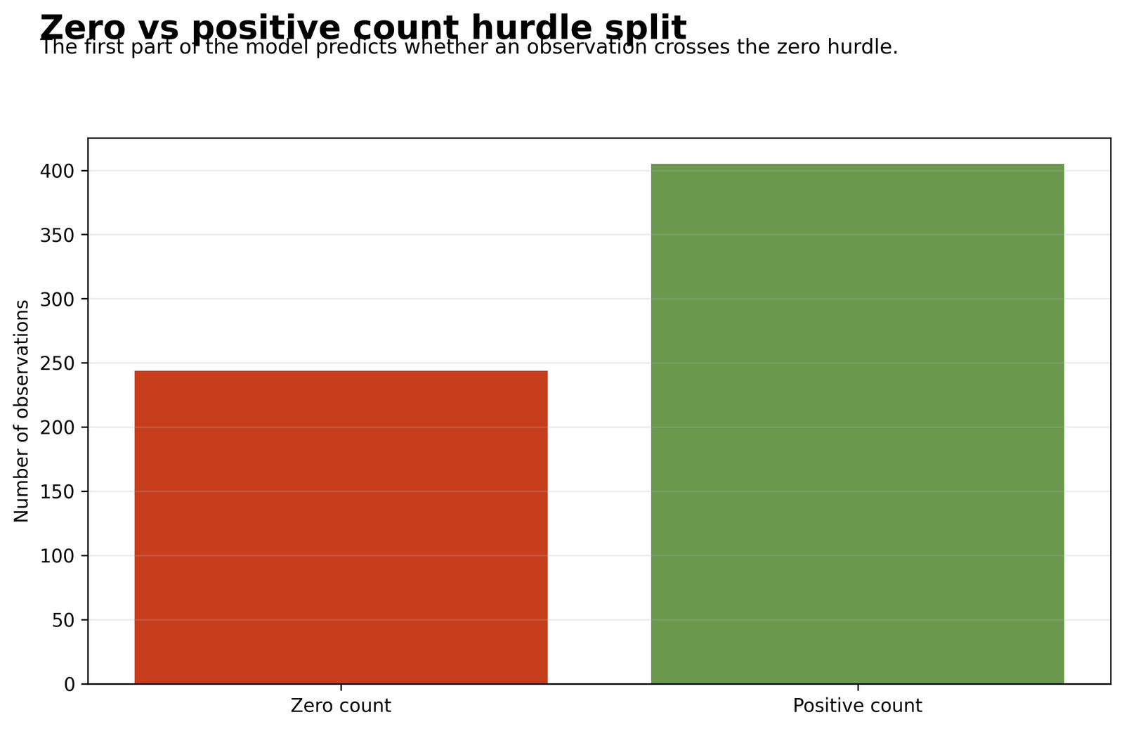
This chart defines the response for the first model component. Every observation is coded as either zero or above zero.
There are 244 zero cases and 405 positive cases. The zero rate is 37.596%, and the positive rate is 62.404%.
A classifier that predicts every observation as positive would already be correct 62.4% of the time. The SPSS logistic model reaches 65.5% accuracy, so classification gains are modest.
Do not judge the binary component by accuracy alone. Review odds ratios, predicted probabilities, calibration, sensitivity and specificity.
Chart 3: Observed Counts Versus Combined Hurdle Predictions
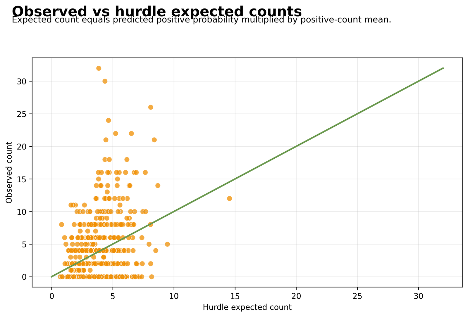
This is the most important overall prediction chart because it recombines the binary and positive-count processes on the original count scale.
Observed counts range from 0 to 32. Most expected counts lie approximately between 1 and 8, with the largest fitted values near 15.
The model captures the central count pattern but compresses the upper tail. High observed counts are frequently above the agreement line, indicating underprediction.
Evaluate a hurdle negative-binomial model, nonlinear predictor effects and influential high-count observations. Compare out-of-sample MAE, RMSE and count calibration.
Chart 4: Residuals Versus Expected Counts
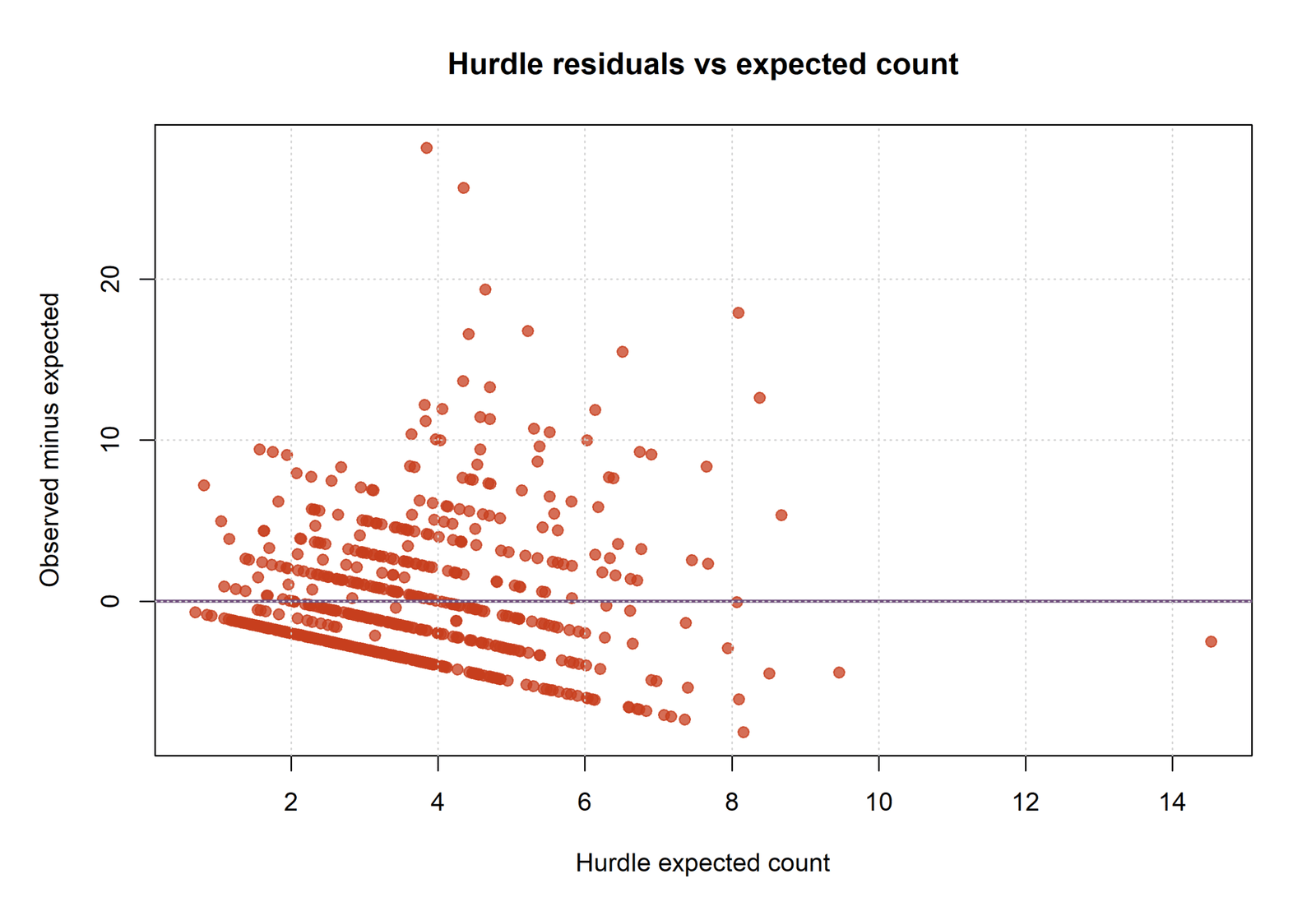
Residuals equal observed count minus combined expected count. Positive residuals indicate underprediction; negative residuals indicate overprediction.
Large positive residuals exceed 20, while negative residuals extend to roughly -7. Several descending bands appear because observed counts are integers.
Residual spread grows for some fitted values, and the long positive tail remains insufficiently modelled. This agrees with the positive-model Pearson dispersion of 3.0749.
Inspect randomized quantile or Pearson residuals, compare hurdle-Poisson with hurdle-negative-binomial, and review high-leverage cases separately.
Chart 5: Odds Ratios for Crossing the Hurdle
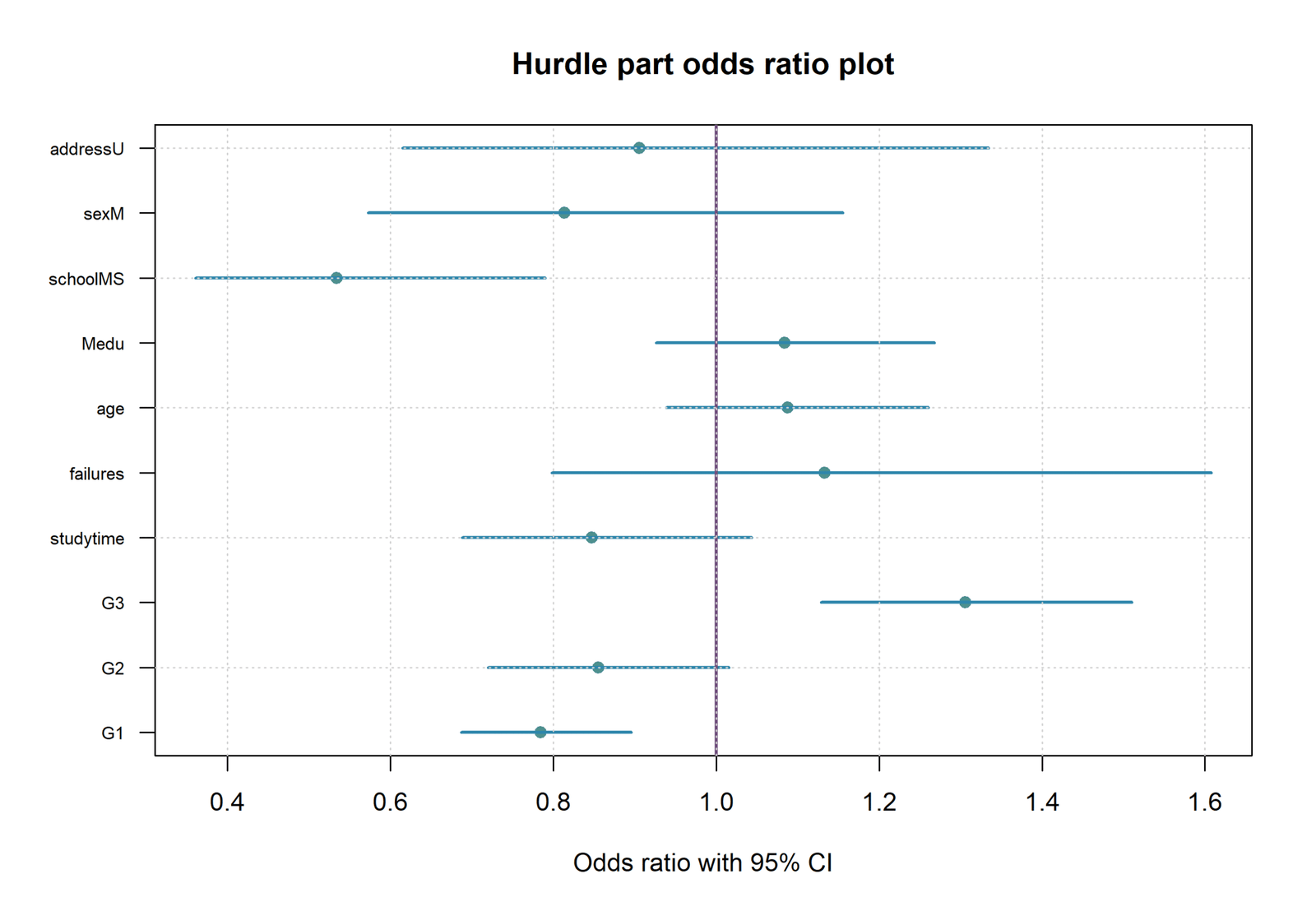
This forest plot belongs only to the binary component. It answers who is more or less likely to have any positive count.
school_MS OR = 0.5339, 95% CI [0.3607, 0.7903]; G1 OR = 0.7846, CI [0.6871, 0.8960]; and G3 OR = 1.3058, CI [1.1290, 1.5103]. These intervals exclude 1.
MS students have approximately 46.61% lower odds of a positive count than GP students. Each additional G1 point is associated with 21.54% lower odds, while each additional G3 point is associated with 30.58% higher odds.
Translate important odds ratios into predicted probabilities for realistic student profiles. Odds ratios should not be described as direct probability changes.
Chart 6: Rate Ratios Among Positive Counts
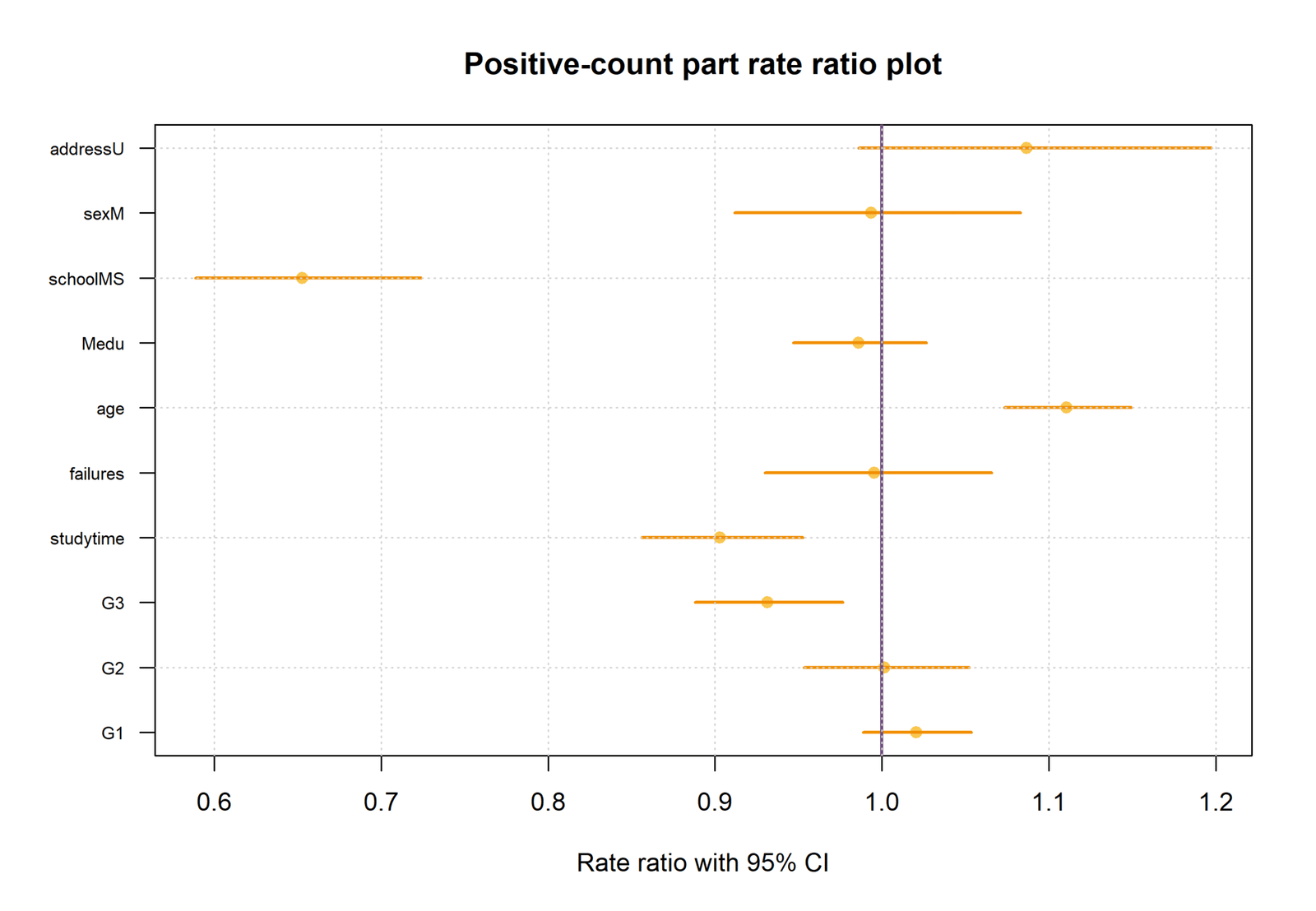
This forest plot belongs to the second model component. It does not describe whether a count is zero; it describes the positive count after the hurdle has been crossed.
school_MS RR = 0.6528, 95% CI [0.5887, 0.7239]; G3 RR = 0.9313, CI [0.8880, 0.9767]; studytime RR = 0.9029, CI [0.8558, 0.9525]; and age RR = 1.1108, CI [1.0733, 1.1495].
Among positive cases, MS has a 34.72% lower expected count, each higher studytime category corresponds to a 9.71% lower expected count, and each additional year of age corresponds to an 11.08% higher count.
Keep these interpretations conditional on a positive count. Do not apply the rate ratio directly to the full sample without also considering the binary component.
Chart 7: Observed and Expected Counts Across G1
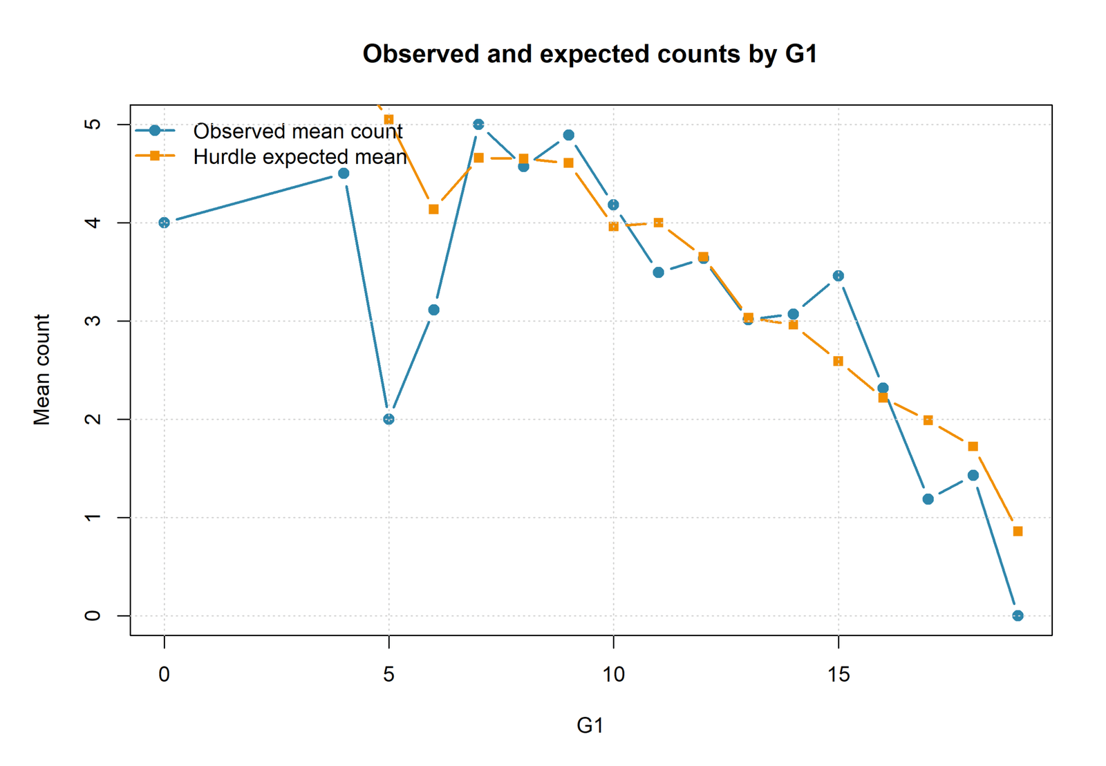
This chart translates the two-part model into an interpretable predictor profile. It compares observed and expected mean counts at each G1 value.
At G1 = 0, observed mean is about 4 and expected mean about 6. At G1 = 5, observed mean is about 2 and expected mean about 5. Through G1 values 7–14, the two lines are generally much closer.
The model follows the central predictor range better than sparse edge values. At G1 = 19, the observed mean is 0 while expected count remains near 0.9.
Add sample sizes or confidence bands by G1. Sparse predictor levels should not drive conclusions about calibration or nonlinear effects.
Chart 8: Predicted Probability of a Positive Count
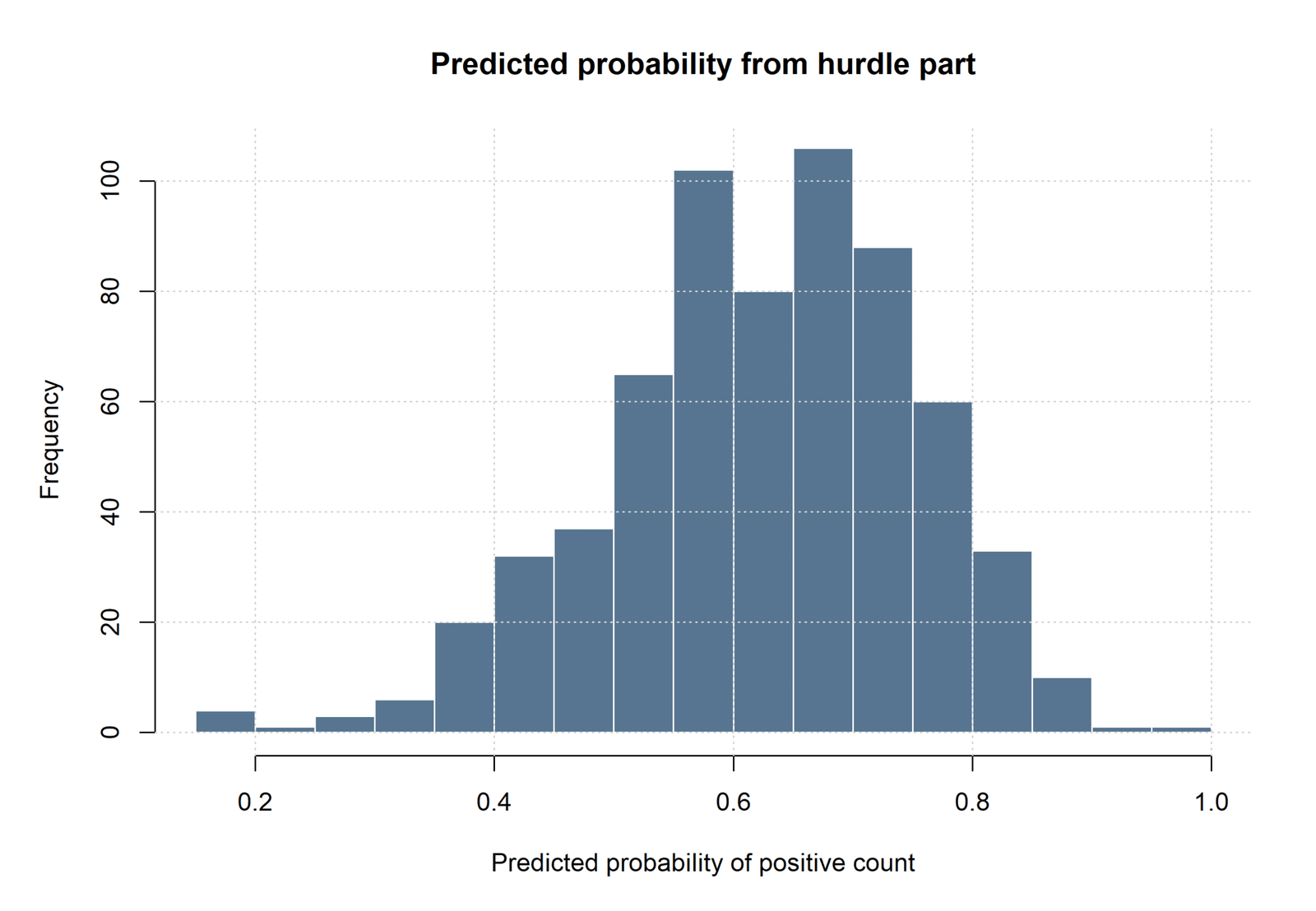
This distribution summarizes how confidently the binary component separates zero and positive observations.
Predicted positive probabilities extend approximately from 0.10 to 0.90. Most observations fall between 0.50 and 0.80, with the greatest concentration around 0.60–0.70.
The model rarely assigns extremely confident probabilities. That limited separation is consistent with the small accuracy gain from 62.4% baseline prevalence to 65.5% SPSS classification accuracy.
Report calibration and probability-based metrics, not accuracy alone. For applied decisions, choose a classification threshold based on costs rather than defaulting automatically to 0.50.
R Charts: Two Charts Followed by Two Matching Explanation Boxes
Each group first displays two R charts side by side. Directly underneath, two explanation boxes appear in the same left-to-right order, so each explanation aligns with the chart immediately above it.
R Chart 1: Count Distribution
R reproduces 244 zeros, 405 positive observations, overall mean 3.6595, and positive-count mean 5.8642. The positive variance is 21.583.
R Chart 2: Zero–Positive Split
The binary hurdle outcome contains 37.596% zeros and 62.404% positive observations.
R Chart 3: Observed vs Expected Counts
Observed counts extend from 0 to 32. Most combined expected counts remain between approximately 1 and 8, with the highest predictions near 15.
R Chart 4: Residuals vs Expected Counts
Positive residuals exceed 20, while negative residuals reach roughly -7. Discrete diagonal bands occur because observed counts are integers.
R Chart 5: Binary Odds Ratios
school_MS OR = 0.5339, G1 OR = 0.7846, and G3 OR = 1.3058. Their 95% confidence intervals exclude 1.
R Chart 6: Positive-Count Rate Ratios
school_MS RR = 0.6528, G3 RR = 0.9313, studytime RR = 0.9029, and age RR = 1.1108.
R Chart 7: Calibration Across G1
Observed and expected means are close through much of the central G1 range. Larger discrepancies appear around G1 = 0, 5, and 19.
R Chart 8: Positive-Probability Distribution
Most predicted probabilities fall between 0.50 and 0.80, with the greatest concentration around 0.60–0.70.
Complete Coefficient Results
Binary hurdle component: odds of a positive count
| Term | B | Odds ratio | 95% OR CI | p-value | Interpretation |
|---|---|---|---|---|---|
| Intercept | 0.9936 | 2.7009 | 0.1920–37.9990 | .4614 | Not significant |
| school: MS vs GP | -0.6276 | 0.5339 | 0.3607–0.7903 | .0017 | Lower positive odds |
| sex: M vs F | -0.2063 | 0.8136 | 0.5729–1.1553 | .2489 | Not significant |
| address: U vs R | -0.0988 | 0.9059 | 0.6149–1.3346 | .6172 | Not significant |
| G1 | -0.2425 | 0.7846 | 0.6871–0.8960 | .0003 | Lower positive odds |
| G2 | -0.1562 | 0.8553 | 0.7201–1.0160 | .0752 | Not significant |
| G3 | 0.2668 | 1.3058 | 1.1290–1.5103 | .0003 | Higher positive odds |
| studytime | -0.1657 | 0.8473 | 0.6880–1.0435 | .1189 | Not significant |
| failures | 0.1250 | 1.1331 | 0.7985–1.6080 | .4840 | Not significant |
| age | 0.0841 | 1.0877 | 0.9386–1.2606 | .2637 | Not significant |
| Medu | 0.0806 | 1.0840 | 0.9265–1.2682 | .3141 | Not significant |
Positive-count component: expected count among positive observations
| Term | B | Rate ratio | 95% RR CI | p-value | Interpretation |
|---|---|---|---|---|---|
| Intercept | 0.8712 | 2.3897 | 1.2608–4.5294 | .0076 | Significant |
| school: MS vs GP | -0.4265 | 0.6528 | 0.5887–0.7239 | <.001 | Lower positive mean |
| sex: M vs F | -0.0064 | 0.9937 | 0.9116–1.0831 | .8850 | Not significant |
| address: U vs R | 0.0831 | 1.0867 | 0.9861–1.1975 | .0933 | Not significant |
| G1 | 0.0205 | 1.0207 | 0.9888–1.0538 | .2064 | Not significant |
| G2 | 0.0016 | 1.0016 | 0.9532–1.0524 | .9494 | Not significant |
| G3 | -0.0712 | 0.9313 | 0.8880–0.9767 | .0034 | Lower positive mean |
| studytime | -0.1022 | 0.9029 | 0.8558–0.9525 | .0002 | Lower positive mean |
| failures | -0.0045 | 0.9955 | 0.9300–1.0657 | .8970 | Not significant |
| age | 0.1050 | 1.1108 | 1.0733–1.1495 | <.001 | Higher positive mean |
| Medu | -0.0141 | 0.9860 | 0.9468–1.0267 | .4939 | Not significant |
Combined Expected Counts and Practical Prediction
What the binary prediction contributes
- A probability between 0 and 1.
- Strongly influenced by school, G1 and G3.
- Moderate separation, with most probabilities between 0.50 and 0.80.
What the count prediction contributes
- An expected positive count greater than zero.
- Strongly influenced by school, G3, studytime and age.
- Positive-tail uncertainty larger than a Poisson variance allows.
Suppose two students have the same positive-count mean but different hurdle probabilities. The student with the larger probability has the larger unconditional expected count. Conversely, a high probability can be offset by a low conditional count mean.
Diagnostics and Model Choice
Binary component diagnostics
- SPSS model χ²(14) = 49.758, p < .001
- Nagelkerke R² = .101
- Hosmer–Lemeshow p = .447
- Classification accuracy = 65.5%
- Baseline positive prevalence = 62.4%
Positive-count diagnostics
- Python/R Pearson dispersion = 3.0749
- SPSS Pearson chi-square/df = 3.000
- SPSS deviance/df = 2.627
- Upper-tail counts are underpredicted
- Hurdle-negative-binomial sensitivity is required
SPSS, Python, R and Excel Workflows
Python
Fits a binomial GLM for hurdle_positive and a Poisson GLM on positive rows, then combines predictions.
- Eight charts
- Odds-ratio and rate-ratio tables
- Dispersion and residual diagnostics
R
Reproduces the same two-part specification and validates coefficients, predictions and chart conclusions.
- Independent coefficient validation
- Pearson dispersion
- Prediction and calibration outputs
SPSS
Uses LOGISTIC REGRESSION for the hurdle gate and GENLIN Poisson with Pearson scaling for positive counts.
- Expanded predictor set
- Classification and goodness-of-fit output
- Pearson scale = 3.000
Excel
Demonstrates the calculation chain with 40 rows and formula-driven hurdle probabilities, positive means, expected counts and residuals.
- 9 zeros and 31 positives
- Mean observed count = 5.2
- Mean expected count = 1.9151
Code: Expand Only the Software You Need
Python Hurdle Model code
import numpy as np
import pandas as pd
import statsmodels.formula.api as smf
import statsmodels.api as sm

df = pd.read_csv("dataset.csv")
df["hurdle_count"] = np.maximum(np.rint(df["absences"]), 0).astype(int)
df["hurdle_positive"] = (df["hurdle_count"] > 0).astype(int)

formula_h = (
    "hurdle_positive ~ G1 + G2 + G3 + studytime + failures"
    " + age + Medu + C(school) + C(sex) + C(address)"
)
formula_c = (
    "hurdle_count ~ G1 + G2 + G3 + studytime + failures"
    " + age + Medu + C(school) + C(sex) + C(address)"
)

logit = smf.glm(
    formula_h, data=df, family=sm.families.Binomial()
).fit()

positive = df[df["hurdle_count"] > 0].copy()
count = smf.glm(
    formula_c, data=positive, family=sm.families.Poisson()
).fit()

df["positive_probability"] = logit.predict(df)
df["positive_mean"] = count.predict(df)
df["expected_count"] = (
    df["positive_probability"] * df["positive_mean"]
)

pearson_dispersion = (
    np.sum(count.resid_pearson ** 2) / count.df_resid
)
R Hurdle Model code
df <- read.csv("dataset.csv", stringsAsFactors = TRUE)
df$hurdle_count <- pmax(round(df$absences), 0)
df$hurdle_positive <- as.integer(df$hurdle_count > 0)

hurdle_fit <- glm(
  hurdle_positive ~ G1 + G2 + G3 + studytime + failures +
    age + Medu + school + sex + address,
  data = df,
  family = binomial(link = "logit")
)

positive_df <- subset(df, hurdle_count > 0)

count_fit <- glm(
  hurdle_count ~ G1 + G2 + G3 + studytime + failures +
    age + Medu + school + sex + address,
  data = positive_df,
  family = poisson(link = "log")
)

df$positive_probability <- predict(
  hurdle_fit, newdata = df, type = "response"
)
df$positive_mean <- predict(
  count_fit, newdata = df, type = "response"
)
df$expected_count <-
  df$positive_probability * df$positive_mean

pearson_dispersion <-
  sum(residuals(count_fit, type = "pearson")^2) /
  df.residual(count_fit)
SPSS Hurdle Model syntax
COMPUTE hurdle_count = RND(MAX(absences,0)).
COMPUTE hurdle_positive = (hurdle_count > 0).
EXECUTE.

LOGISTIC REGRESSION VARIABLES hurdle_positive
 /METHOD=ENTER G1 G2 G3 studytime failures age Medu Fedu health
  school_MS sex_M address_U higher_yes internet_yes
 /PRINT=CI(95) GOODFIT.

TEMPORARY.
SELECT IF hurdle_count > 0.
GENLIN hurdle_count WITH G1 G2 G3 studytime failures age
 Medu Fedu health school_MS sex_M address_U higher_yes internet_yes
 /MODEL G1 G2 G3 studytime failures age Medu Fedu health
  school_MS sex_M address_U higher_yes internet_yes INTERCEPT=YES
 DISTRIBUTION=POISSON LINK=LOG
 /CRITERIA SCALE=PEARSON
 /PRINT CPS DESCRIPTIVES MODELINFO FIT SUMMARY SOLUTION.

OUTPUT EXPORT
 /CONTENTS EXPORT=ALL LAYERS=PRINTSETTING MODELVIEWS=PRINTSETTING
 /PDF DOCUMENTFILE=
'D:\DATA ANALYSIS\H Regression Tests and Models\Hurdle Model\SPSS_Output\pdf\Hurdle-Model-SPSS-Output.pdf'.
Excel calculation logic
Positive probability:
=1/(1+EXP(-BinaryLinearPredictor))

Positive-count mean:
=EXP(PositiveCountLinearPredictor)

Combined expected count:
=PositiveProbability*PositiveCountMean

Raw residual:
=ObservedCount-ExpectedCount

Squared residual:
=RawResidual^2
The Excel coefficients are teaching values. Use fitted Python, R or SPSS coefficients for final inferential reporting.
Advanced Interpretation and Extensions
The essential analysis remains visible above. The following topics are collapsed so advanced material does not interrupt the main reading path.
How the binary and count likelihoods combine
The Hurdle Model likelihood has two non-overlapping contributions. A zero observation contributes only the probability of not crossing the hurdle. A positive observation contributes the probability of crossing the hurdle multiplied by the probability of its positive value under the truncated count distribution.
This separation means that the binary and positive-count coefficient blocks answer independent questions, even when the same predictors are placed in both components. Their log-likelihood contributions can be added to produce the complete model log likelihood.
- For Y = 0: contribution = 1 − P(Y > 0).
- For Y > 0: contribution = P(Y > 0) × truncated count probability.
- The zero-truncation denominator removes the probability mass that an ordinary Poisson or negative-binomial distribution would place at zero.
Why predicted counts can understate extreme observations
Regression predictions estimate conditional means, not the largest value that can occur. A few observations with counts near 20–32 can therefore lie well above a fitted mean even when the central model is useful.
In this analysis, the problem is stronger than ordinary random variation because the positive Poisson component assumes variance equal to its mean. The observed positive variance of 21.583 is much larger than the positive mean of 5.8642.
- A negative-binomial count component introduces a dispersion parameter.
- Nonlinear predictors may improve the mean structure.
- Influence diagnostics identify whether a few cases dominate coefficients.
- Prediction intervals should describe the full conditional count distribution, not only the fitted mean.
How to calculate predictor-specific combined effects
A predictor’s unconditional expected-count effect must pass through both components. Calculate predictions at two meaningful predictor values while holding other variables at a defined profile, then compare the recombined expected counts.
- Predict the positive probability at value A and value B.
- Predict the positive-count mean at value A and value B.
- Multiply each probability by its corresponding positive mean.
- Report the absolute difference, ratio or percentage change in the combined expected count.
This approach is especially important for G3 because it increases positive-count probability but decreases positive-count magnitude. Neither component alone describes its overall expected-count relationship.
Choosing realistic prediction profiles
Do not interpret an intercept profile containing zero values for G1, G2, G3, studytime, age and education as though it represented a typical student. Use observed or substantively meaningful covariate profiles.
- Use medians or common categories for a representative profile.
- Show contrasts for GP versus MS while holding academic predictors fixed.
- Plot G3 or G1 across its observed range rather than extrapolating.
- Average row-level predictions when a population-average result is required.
Average marginal predictions are often clearer than exponentiated intercepts because they remain within the observed covariate distribution.
Assessing the binary component beyond classification accuracy
Classification accuracy depends on the selected probability threshold and the prevalence of positive counts. With 62.404% positives, predicting every case as positive already achieves 62.4% accuracy.
A 65.5% model accuracy therefore represents only a 3.1 percentage-point improvement over the prevalence baseline. Additional assessment should include:
- Calibration plots and calibration slope.
- Brier score for probability accuracy.
- ROC AUC for ranking ability.
- Sensitivity and specificity at decision-relevant thresholds.
- Precision and recall when one class is more important.
Assessing the positive component beyond Pearson dispersion
Pearson dispersion is a summary warning, not a complete model diagnostic. A value near 3 means that the observed residual variation is much larger than the Poisson model expects, but it does not identify the precise source.
- Compare zero-truncated Poisson and negative-binomial likelihood criteria.
- Inspect randomized quantile residuals and rootograms.
- Check whether variance differs by school or fitted-count range.
- Review the upper tail separately from central counts.
- Test nonlinear terms and interactions suggested before model fitting.
If the negative-binomial model removes the dispersion pattern without destabilizing coefficients, it is usually more suitable for final reporting.
How reference categories affect interpretation
The reported school, sex and address effects compare each named category with its omitted reference. Here, school_MS compares MS with GP, sex_M compares male with female, and address_U compares urban with rural.
Changing a reference category changes the coefficient labels and intercept but does not change fitted probabilities, expected counts or overall model fit. The public report should always state references beside the variables.
Model specification differences across software
Python and R use G1, G2, G3, studytime, failures, age, Medu, school, sex and address in both components. The SPSS workflow additionally includes Fedu, health, higher-education intention and internet access.
SPSS coefficient values and p-values are therefore not expected to match the smaller Python/R specification exactly. Cross-software comparison should focus on direction, scale, data coding and overlapping predictors rather than demanding identical numerical output from different formulas.
Likelihood structure of the Hurdle Model
For an observation equal to zero, the likelihood contribution comes entirely from the binary component. For a positive observation, the likelihood contribution combines the probability of crossing the hurdle with the zero-truncated count probability.
Because the two parameter blocks are variation-independent under standard formulations, the binary and positive components can often be estimated separately while still defining one coherent likelihood.
Zero-truncated Poisson interpretation
The ordinary Poisson mean parameter is not identical to the conditional mean after truncation. For Poisson rate λ, the positive conditional mean equals λ/(1-e-λ).
This distinction matters when translating fitted log-rate coefficients into expected positive counts and when reconstructing unconditional predictions.
Model comparison beyond AIC
- Compare observed and predicted zero proportions.
- Compare the full count probability distribution, not only the mean.
- Assess binary calibration and discrimination.
- Assess positive-count residuals, dispersion and tail fit.
- Use cross-validated log score, MAE and RMSE.
- Choose the model whose data-generating interpretation is scientifically credible.
Interpreting school across both components
MS school membership lowers the odds of any positive count and lowers the expected magnitude among positive cases. The combined unconditional difference is therefore reinforced across both parts.
The exact combined percentage difference is not obtained by adding 46.61% and 34.72%. It must be calculated from predicted probabilities and positive means for defined covariate profiles.
Interpreting G3 across both components
G3 increases the odds of crossing the hurdle by 30.58% per point but reduces the positive-count mean by 6.87% per point. These effects operate in opposite directions.
The unconditional effect may be positive, negative or non-monotonic depending on the baseline probability and count mean. Plotting predicted expected counts across G3 is preferable to summarizing one overall percentage.
Interpreting studytime and age
studytime is not statistically significant in the binary component but is associated with a 9.71% lower positive count per category. Age is not significant in the binary component but is associated with an 11.08% higher positive count per year.
These variables appear to influence magnitude after occurrence more than the occurrence decision itself.
Binary probability calibration
Calibration asks whether observations assigned a 0.70 probability become positive about 70% of the time. Group predictions into probability bins, compare observed and predicted rates, and calculate a calibration intercept and slope when possible.
Moderate fitted probabilities and only a small accuracy gain make calibration more informative than a single classification threshold.
Positive-count calibration
Compare observed and expected positive means across quantiles of fitted count, key predictors and relevant groups. A model may have an acceptable average mean while underpredicting the upper tail.
Randomized quantile residuals and rootograms are useful because ordinary raw residual bands are an expected consequence of discrete outcomes.
Hurdle Model vs Zero-Inflated Model
- A hurdle model assigns every zero to the binary gate and uses a zero-truncated distribution for positives.
- A zero-inflated model mixes an always-zero process with an ordinary count distribution that may also generate zeros.
- Choose between them using the substantive data-generating story, predictive performance, diagnostics and model comparison.
Hurdle Poisson vs Hurdle Negative Binomial
- The Poisson component assumes conditional mean equals conditional variance.
- The positive-count Pearson dispersion of 3.0749 indicates substantial extra-Poisson variation.
- A zero-truncated negative-binomial component can model an additional dispersion parameter and should be a primary sensitivity model.
Offsets and Exposure
- Use an offset when counts arise over unequal exposure times, populations or opportunities.
- The count equation includes log(exposure) with its coefficient fixed at 1.
- The binary component may also require exposure-related predictors because longer exposure can increase the chance of crossing the hurdle.
Interactions and Nonlinear Terms
- A predictor may interact with school or another characteristic differently in the binary and count components.
- Continuous predictors such as G1, G3 and age may need polynomial terms or splines.
- Plot combined expected counts because separate component coefficients do not directly show the total interaction effect.
Robust Standard Errors, Clustering and Dependence
- Ordinary two-part estimates assume independent observations.
- Clustered or repeated data require cluster-aware covariance, generalized estimating equations, random effects or Bayesian multilevel hurdle models.
- A robust covariance corrects uncertainty but does not fix an incorrect positive-count distribution.
Outliers and Influence
- High counts can dominate the positive component, while unusual zero/positive classifications can dominate the binary component.
- Inspect component-specific leverage, Pearson residuals, deviance residuals and case-deletion sensitivity.
- Do not remove high counts merely because the fitted Poisson model underpredicts them.
Prediction Validation
- Use training/test splits or resampling that preserves clustering and outcome prevalence.
- Evaluate binary calibration and discrimination, positive-count error, and the combined count distribution.
- A model can classify zeros well but predict positive magnitudes poorly, or the reverse.
Uncertainty for the Combined Mean
- The expected count is the product of two estimated quantities.
- A confidence interval based only on one component is incomplete.
- Bootstrap both model fits together or simulate jointly from their estimated coefficient distributions.
Sensitivity to the Definition of Zero
- The worked outcome defines zero using rounded non-negative absences.
- A different threshold or measurement rule changes both the binary prevalence and the positive-count sample.
- Report the construction rule explicitly and repeat the analysis when plausible definitions differ.
Bayesian and Multilevel Hurdle Models
- Bayesian models can estimate both components jointly and produce posterior distributions for combined predictions.
- Multilevel hurdle models add group-specific intercepts or slopes to one or both components.
- Priors and random-effect structures must be justified; complexity cannot replace adequate data.
APA-Style Reporting
Publication Checklist and Common Mistakes
Report these items
- Exact count construction and zero definition
- Zero count, positive count and zero percentage
- Predictors and reference categories in each component
- Odds ratios and rate ratios with 95% confidence intervals
- Combined expected-count formula
- Binary calibration and classification context
- Positive-count dispersion and residual diagnostics
- Poisson versus negative-binomial sensitivity
Avoid these mistakes
- Interpreting an odds ratio as a rate ratio
- Applying count-part results to zero observations
- Calling every observed zero a structural zero
- Ignoring overdispersion above 3
- Using accuracy without the 62.4% prevalence baseline
- Reporting separate predictions without recombining them
- Assuming a significant p-value implies large predictive value
- Repeating identical charts without added interpretation
Downloads
R Hurdle Model ReportIndependent validation of both components and combined predictions.
SPSS Hurdle Model OutputLogistic and positive-count GENLIN output.
Worked Excel FileFormula-based teaching workbook for the two-part calculation.
Frequently Asked Questions
What is a Hurdle Model?
A Hurdle Model is a two-part model: a binary component predicts zero versus positive, and a zero-truncated count component predicts the magnitude of positive counts.
Why not use one Poisson regression?
The outcome has 37.596% zeros, a long positive tail and positive-count dispersion of 3.0749. One equidispersed process is too restrictive.
What does the binary component predict?
It predicts the probability that hurdle_count is greater than zero.
What does the positive-count component predict?
It predicts the expected count among observations whose count is already positive.
How is the overall expected count calculated?
Multiply the predicted positive probability by the predicted positive-count mean.
How do I interpret an odds ratio below 1?
It indicates lower odds of crossing from zero to a positive count, holding the other binary-model predictors constant.
How do I interpret a rate ratio below 1?
It indicates a lower expected positive count among cases above zero, holding the count-model predictors constant.
Which predictors were important in the binary component?
school_MS, G1 and G3 had confidence intervals that excluded an odds ratio of 1.
Which predictors were important in the positive component?
school_MS, G3, studytime and age had confidence intervals that excluded a rate ratio of 1.
What does Pearson dispersion of 3.0749 mean?
The positive-count variability is much larger than a Poisson model expects, supporting a negative-binomial sensitivity model.
Is a Hurdle Model the same as a zero-inflated model?
No. A hurdle model assigns all zeros to the binary gate. A zero-inflated model allows both structural and sampling zeros.
Why can one predictor have opposite effects in the two components?
Occurrence and magnitude are separate mechanisms. A variable may increase the chance of a positive count while reducing the count among positive observations.
Can I interpret odds ratios as probability changes?
No. Odds ratios multiply odds. Use predicted probabilities to describe absolute probability changes.
Can SPSS fit a Hurdle Model?
SPSS can fit the two components separately with LOGISTIC REGRESSION and GENLIN, then combine predictions.
Can Excel fit the final Hurdle Model?
Excel is useful for transparent formula demonstrations. Python, R or SPSS should provide the final fitted coefficients and inferential output.
What is the next model to test?
A hurdle negative-binomial model is the main next step because the positive-count dispersion is substantially above 1.
Final Hurdle Model Conclusion
The count outcome is best understood as two linked processes. The first determines whether the observation remains at zero or crosses into the positive range. The second determines how large the count becomes after that transition.
School, G1 and G3 explain important differences in crossing the hurdle. School, G3, studytime and age explain important differences in positive-count magnitude. The combined prediction charts show useful central calibration but substantial upper-tail underprediction.

