
Poisson Regression: Formula, Interpretation, Python, R, SPSS and Excel Guide
Learn how Poisson Regression models a conditional expected count, converts coefficients into incidence rate ratios, checks equidispersion, diagnoses residual problems, and reproduces one verified 649-case analysis across four software environments.
9 predictors
AIC 3009.7990
Dispersion 0.243139
Poisson Regression Model Overview
Poisson Regression is a generalized linear model for a nonnegative count response. It connects predictors to the conditional expected count through a logarithmic link: log(μi) = xi′β. Exponentiating the linear predictor gives μi, which is always positive. Exponentiating one coefficient gives an incidence rate ratio, the multiplicative change in the expected count associated with a one-unit predictor increase or a factor contrast.
The method answers a focused research question: how does the conditional expected count differ across predictor values after the other terms are held fixed? In the worked analysis, the outcome is a rounded, nonnegative version of final grade G3. The model asks how its fitted mean changes with G1, G2, studytime, failures, absences, age, school, sex, and address. This is an associational mean question, not proof that any predictor causes the outcome.
Use Poisson Regression when the outcome is a genuine count, observations are independent under the planned covariance model, the conditional mean is appropriately log-linear, and the conditional variance is reasonably close to the conditional mean. The method is particularly natural for events observed over a common exposure or for rates when a verified log exposure offset is included.
Do not use Poisson Regression merely because a variable contains integers. A bounded score, ordinal rating, continuous measure rounded to whole numbers, proportion, or repeated count may require another model. It is also unsuitable when structural zeros, clustering, strong nonlinearity, or major dispersion failure remain unaddressed. Compare Quasi Poisson Regression, Negative Binomial Regression, Zero-Inflated Poisson Regression, and Generalized Estimating Equations when those conditions matter.
Compared with ordinary linear regression, Poisson Regression uses a positive multiplicative mean and a count probability model instead of a constant additive mean with normally distributed errors. Compared with logistic regression, it predicts an expected count rather than a probability of one binary outcome. Compared with quasi-Poisson, it supplies a complete likelihood and ordinary AIC but fixes the dispersion at one for model-based inference.
The probability model states Yi|Xi ~ Poisson(μi), with E(Yi|Xi) = Var(Yi|Xi) = μi. This equality is equidispersion. It is not an optional detail: it governs the likelihood variance, model-based standard errors, prediction distribution, and the meaning of residual diagnostics.
Supported predictors include numeric covariates, categorical factors, interactions, nonlinear transformations, splines, and offsets. Numeric slopes are interpreted per stated unit. Factor slopes compare a displayed level with its reference. Interactions require conditional rate ratios rather than isolated main-effect readings.
Core assumptions include a nonnegative count outcome, correct exposure unit, independent observations for the displayed likelihood, a suitable log-linked conditional mean, estimable coefficients, no unmodeled structural-zero mechanism, and conditional variance close enough to μ for ordinary standard errors and probability statements. A model may fit the mean well while failing the variance assumption.
The main advantages of Poisson Regression are positive fitted means, natural multiplicative effects, an explicit count likelihood, deviance-based model comparison, and ordinary AIC. Its limitations include sensitivity to dispersion, inability to respect natural upper bounds, vulnerability to clustering and zero inflation, and rate-ratio interpretations that can be misleading when no exposure denominator exists.
The worked scenario contains 649 complete observations and ten estimated parameters: an intercept, six numeric slopes, and three factor contrasts. Null deviance is 745.607271, residual deviance is 247.065469, and AIC is 3009.799014. G2 is the strongest positive predictor, with β = 0.086381 and IRR = 1.090222. The decisive diagnostic is Pearson chi-square 155.365855 on 639 residual degrees of freedom, giving dispersion 0.243139 and strong underdispersion.
Quick Answer
Main Mean-Model Result
- G2 coefficient: 0.086381
- G2 incidence rate ratio: 1.090222
- Ordinary 95% IRR interval: 1.071520 to 1.109250
- One-point G2 increase: approximately 9.02% higher fitted count
Main Diagnostic Result
- Pearson chi-square: 155.365855
- Residual df: 639
- Dispersion: 0.243139
- Conclusion: strong underdispersion, not overdispersion
Table of Contents
- Model Overview
- Quick Answer
- When Poisson Regression Is Needed
- How Poisson Regression Works
- Variables and Data Dictionary
- Verified Results
- Python Chart Stories
- R Chart Pairs
- Coefficient Interpretation
- Predictions and Worked Cases
- Assumptions and Diagnostics
- Python, R, SPSS and Excel
- Reproducible Code
- 26 Advanced Topics
- APA-Style Reporting
- Publication Checklist
- Downloads
- Related Guides
- 16 FAQs
- Conclusion
When Poisson Regression Is Needed
Poisson Regression is needed when the research outcome is a count and the analyst wants to model its conditional expected value as a multiplicative function of predictors. The method is more appropriate than ordinary least squares when negative predictions would be nonsensical, effects are naturally expressed as ratios, and the Poisson probability model is plausible.
In the supplied analysis, the model is used as a worked demonstration because G3 is already integer-valued and nonnegative. The research question is whether the fitted grade-count changes with prior grades, study time, previous failures, absences, age, school, sex, and address. The method provides a clear log-link and rate-ratio lesson, but the bounded score requires explicit caution.
Before fitting Poisson Regression, review the response with Descriptive Statistics and a Frequency Distribution. Confirm the minimum, maximum, zero frequency, exposure unit, group structure, missingness, and whether repeated observations are present. Integer values alone are not sufficient justification.
Appropriate Conditions
- Nonnegative event or count outcome
- Meaningful common exposure or verified offset
- Log-linked conditional mean is plausible
- Observations are independent under the covariance model
- Variance is approximately equal to the mean
- Rate ratios answer the scientific question
Conditions Requiring Another Model
- Strong underdispersion or overdispersion
- Structural-zero or hurdle process
- Natural upper bound central to measurement
- Repeated or clustered observations
- Ordinal categories rather than event counts
- Nonlinear or interaction-rich mean not yet specified
The worked evidence supports a useful conditional mean but rejects equidispersion. That dual result is why the article does not simply label the model “good” or “bad.” The log mean captures grade progression; the ordinary Poisson variance is unsuitable for final inferential confidence.
How Poisson Regression Works
Confirm a nonnegative outcome, exposure unit, factor references, and valid analytic rows.
Set log(μ) equal to the intercept plus numeric terms and factor contrasts.
Choose β values that maximize the Poisson probability of the observed counts.
Interpret IRRs, deviance, Pearson residuals, influence, calibration, and alternatives.
Maximum likelihood estimates β from the complete probability mass function. The log likelihood sums yilog(μi) − μi − log(yi!). The model is normally fitted by iteratively reweighted least squares, which repeatedly updates the coefficient vector until the score and curvature stabilize.
For G2, β = 0.086381. Exponentiation gives 1.090222, so the conditional expected count is multiplied by 1.090222 for a one-point G2 increase. The same effect can be stated as approximately 9.02% higher. The interpretation is conditional on every other predictor and the factor references.
Poisson Regression model fit can be summarized with deviance and AIC because it has a full likelihood. The reduction from null deviance 745.607271 to residual deviance 247.065469 shows that the predictors improve the mean compared with an intercept-only model. AIC 3009.799014 can compare candidate Poisson likelihood models using the same outcome and observations.
Dispersion is checked after the mean is fitted. The Pearson residual is (yi−μ̂i)/√μ̂i. Summing squared Pearson residuals and dividing by residual degrees of freedom gives φ̂. Here 155.365855/639 = 0.243139, contradicting the equality of conditional mean and variance.
Review Generalized Linear Model for the family-link framework, Confidence Interval for interval interpretation, and Standard Error for the role of covariance in coefficient uncertainty.
Variables and Data Dictionary
The verified Poisson Regression model uses 649 complete observations. The outcome is the nonnegative count-like version of G3. Six predictors are entered as numeric one-unit terms, and school, sex, and address are entered through treatment-coded factor contrasts. No offset, weight, interaction, random effect, or nonlinear term appears in the saved equation.
Representative source records used in the fitted design
| Row | G3/count | G1 | G2 | Study time | Failures | Absences | Age | School | Sex | Address |
|---|---|---|---|---|---|---|---|---|---|---|
| 1 | 11 | 0 | 11 | 2 | 0 | 4 | 18 | GP | F | U |
| 2 | 11 | 9 | 11 | 2 | 0 | 2 | 17 | GP | F | U |
| 3 | 12 | 12 | 13 | 2 | 0 | 6 | 15 | GP | F | U |
| 4 | 14 | 14 | 14 | 3 | 0 | 0 | 15 | GP | F | U |
| 5 | 13 | 11 | 13 | 2 | 0 | 0 | 16 | GP | F | U |
| 648 | 10 | 10 | 10 | 1 | 0 | 6 | 17 | MS | M | U |
| 649 | 11 | 10 | 11 | 1 | 0 | 4 | 18 | MS | M | R |
The public article avoids reproducing all 649 design rows. The complete case-level audit remains available in the downloadable software reports and Excel workbook. This keeps the post readable without concealing the analysis inputs.
Verified Poisson Regression Results
The fitted model uses a Poisson family, log link, 649 observations, nine slopes, an intercept, and 639 residual degrees of freedom. It substantially reduces deviance relative to the intercept-only model, but its Pearson dispersion shows that the ordinary variance assumption is not supported.
Ordinary Poisson coefficient and incidence rate-ratio results
| Term | Log-rate β | SE | p | IRR | 95% IRR CI | Reading |
|---|---|---|---|---|---|---|
| Intercept | 1.575261 | 0.179792 | 1.92578 × 10⁻¹⁸ | 4.832001 | 3.396936–6.873319 | Model anchor |
| School: MS vs GP | −0.033380 | 0.027699 | 0.228159 | 0.967171 | 0.916064–1.021129 | Interval includes 1 |
| Sex: M vs F | −0.016781 | 0.024141 | 0.486967 | 0.983359 | 0.937915–1.031005 | Interval includes 1 |
| Address: U vs R | 0.008394 | 0.027100 | 0.756757 | 1.008429 | 0.956264–1.063440 | Interval includes 1 |
| G1 | −0.002184 | 0.009062 | 0.809530 | 0.997818 | 0.980252–1.015699 | Interval includes 1 |
| G2 | 0.086381 | 0.008828 | 1.31095 × 10⁻²² | 1.090222 | 1.071520–1.109250 | Positive association |
| Study time | 0.002714 | 0.014538 | 0.851932 | 1.002717 | 0.974549–1.031700 | Interval includes 1 |
| Failures | −0.040593 | 0.025475 | 0.111071 | 0.960220 | 0.913453–1.009382 | Interval includes 1 |
| Absences | 0.002660 | 0.002617 | 0.309462 | 1.002663 | 0.997534–1.007819 | Interval includes 1 |
| Age | −0.005937 | 0.010293 | 0.564072 | 0.994081 | 0.974228–1.014338 | Interval includes 1 |
Quick Report Downloads
Open the complete software reports before reproducing the worked values.
Python Poisson Regression Charts and Explanations
Each Python chart is explained through its visible pattern, exact values, statistical meaning, and next analytical step. All figures use the same 649 observations and the same Poisson Regression equation.
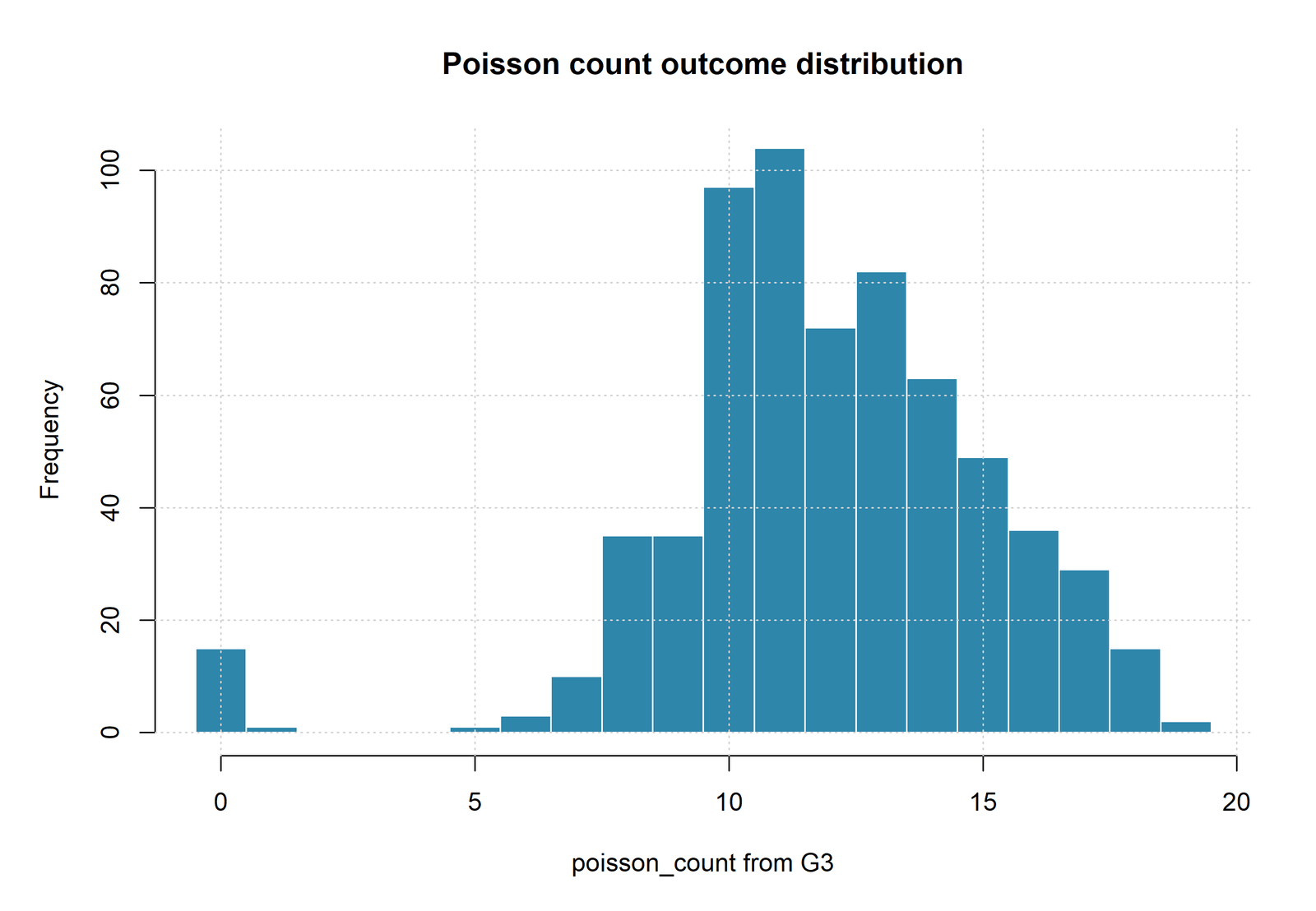
Python Chart 1: Distribution of the Constructed Count
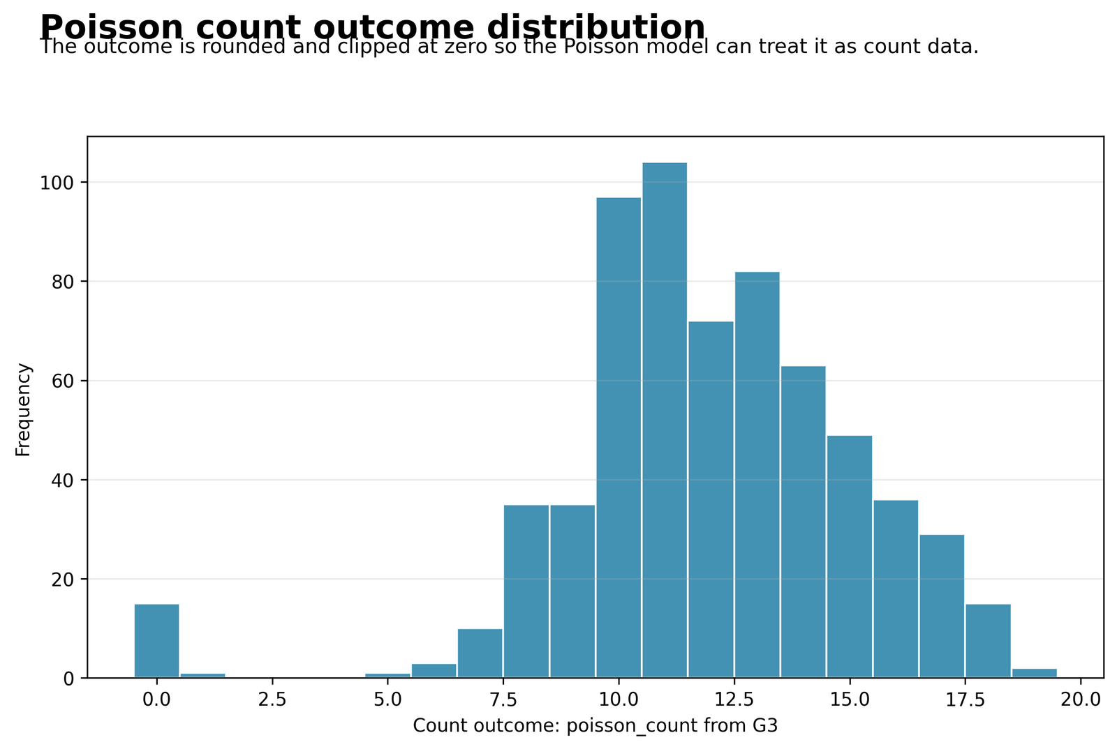
The response occupies a limited educational score range instead of the long right tail typical of an unrestricted event count. Integer outcomes form concentrated bars with a visible lower boundary at zero.
All 649 observations enter the model. The observed mean is approximately 11.9060, and the response is bounded by the grade scale rather than open-ended exposure time.
The coding satisfies the nonnegative-integer requirement, but the measurement process is not a naturally unlimited arrival process. That bounded support helps explain why the residual variation is much smaller than the Poisson variance benchmark.
Use the graph to justify the underdispersion discussion and compare the count representation with continuous or ordinal alternatives before treating the Poisson family as substantively final.
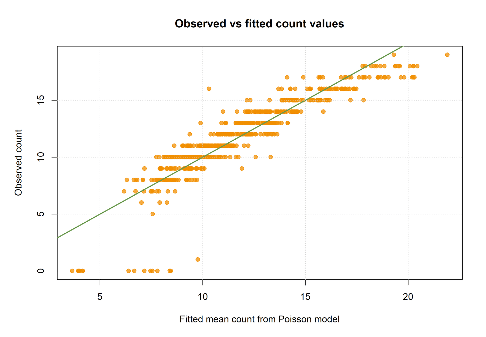
Python Chart 2: Observed Counts Versus Conditional Means
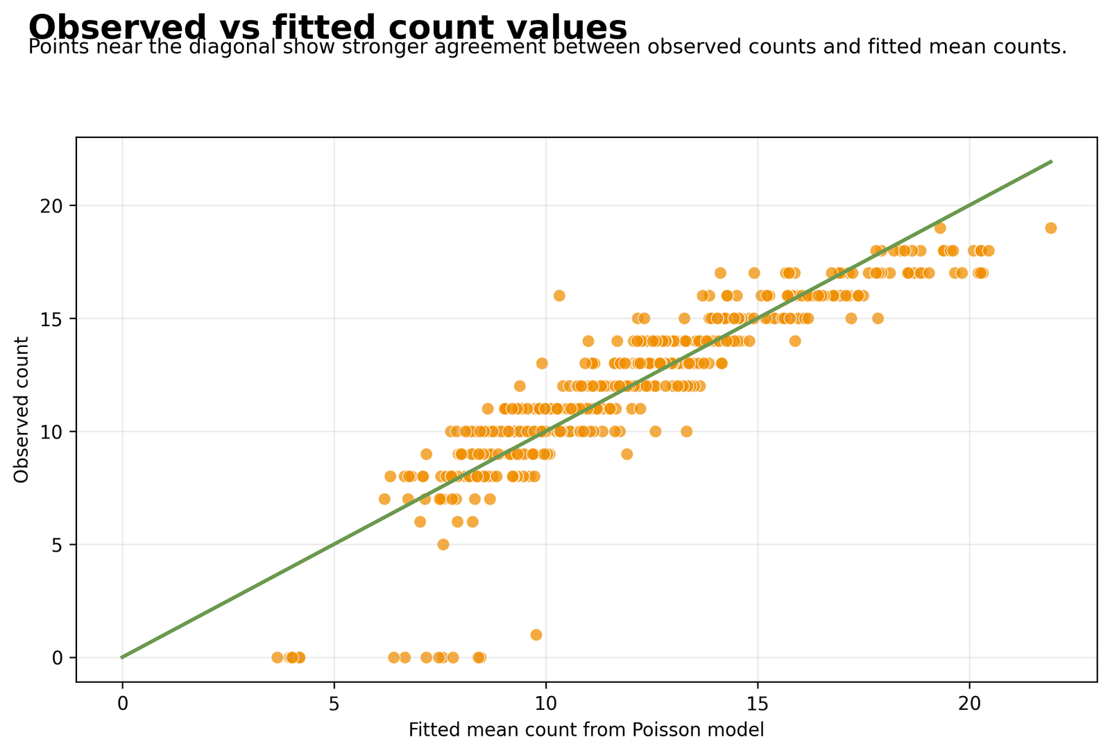
Discrete observations form horizontal bands, while fitted conditional means remain continuous. Most cases track the agreement direction, but low observed outcomes include several large overpredictions.
The fitted mean averages 11.9060, ranges from 3.6519 to 21.9136, and yields in-sample RMSE = 1.4353 and MAE = 0.9372.
Proximity to the identity line assesses the conditional mean, not the equality of conditional mean and variance. A visually useful fit can coexist with a poor Poisson uncertainty model.
Inspect Pearson and deviance residuals, especially the zero-grade cases and the highest fitted values. Slight predictions above the observed score ceiling reveal the limitation of using an unbounded log mean for a bounded grade.
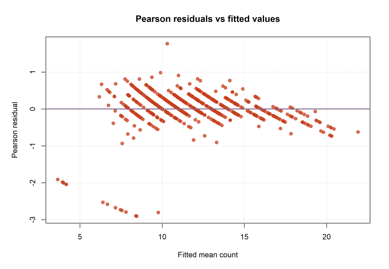
Python Chart 3: Pearson Residuals Versus Fitted Values
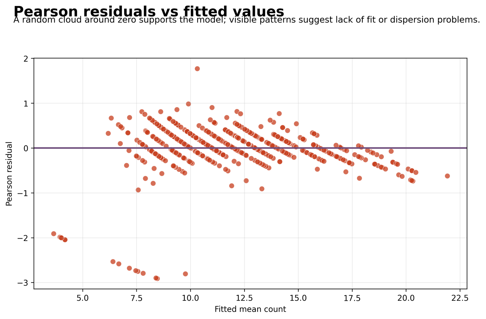
Most residuals are compressed around zero rather than displaying the unit-scale spread expected under equidispersion. Several zero outcomes create a pronounced negative tail.
The squared Pearson residuals sum to 155.365855. Dividing by 639 residual degrees of freedom gives φ̂ = 0.243139. Residuals range from approximately −2.9080 to 1.7711.
The model is underdispersed: residual variation is only about 24.31% of the ordinary Poisson benchmark after accounting for the fitted mean and parameter count.
Do not call this overdispersion. Compare the ordinary results with Quasi Poisson Regression and check whether one scalar variance correction is scientifically adequate.
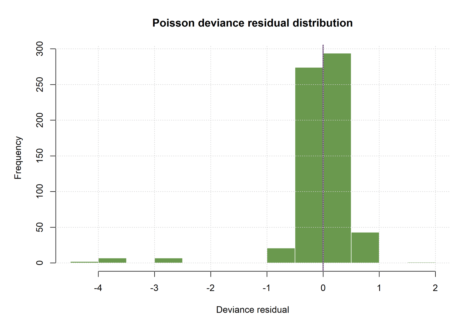
Python Chart 4: Deviance Residual Distribution
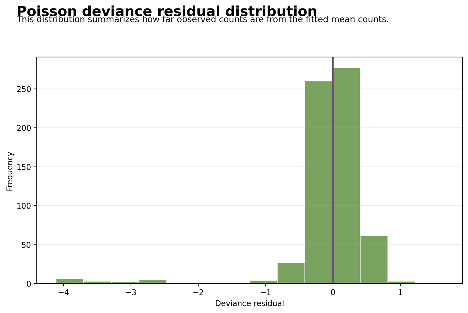
The center is concentrated near zero, but the distribution has a longer negative tail. Zero or very low observed grades are the hardest cases for the fitted conditional mean.
Deviance residuals range from approximately −4.1126 to 1.6372. Case 164 has observed count 0, fitted mean 8.4565, and deviance residual −4.1126.
The residual tail identifies localized lack of fit that the aggregate deviance does not explain by itself. The bounded grade process produces behavior different from an unrestricted Poisson event count.
Trace extreme residuals back to source rows, verify their coding, and perform sensitivity analysis. Legitimate difficult observations should not be deleted merely because they challenge the fitted distribution.
Python Chart 5: Adjusted Incidence Rate Ratios
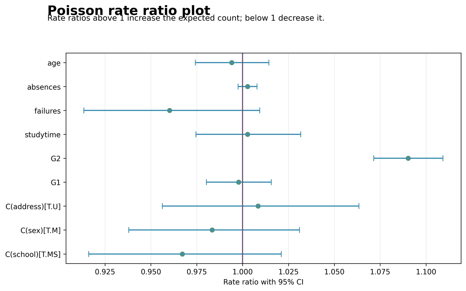
G2 is clearly above the no-change reference of one. Most other predictor intervals overlap one once the full predictor set is held constant.
G2 IRR = 1.090222, 95% CI [1.071520, 1.109250]. School MS IRR = 0.967171, failures IRR = 0.960220, and absences IRR = 1.002663.
A rate ratio above one indicates a multiplicative increase in the fitted conditional mean; a value below one indicates a decrease. Interval width reflects ordinary unit-dispersion Poisson uncertainty.
Interpret each marker with its predictor unit and factor reference. Then compare interval conclusions with the Pearson-scaled sensitivity analysis rather than mixing ordinary and scaled statistics.
Python Chart 6: Equidispersion Check
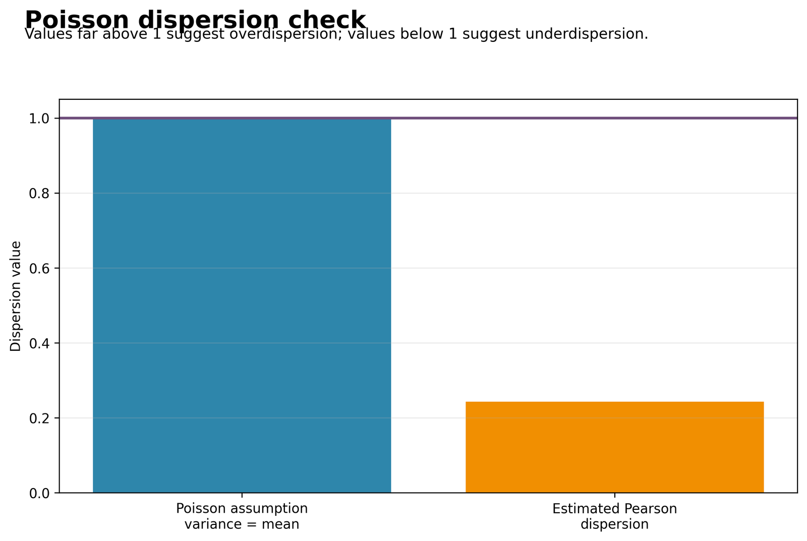
The estimated dispersion bar is far below the reference line at one. The visual gap is large enough that equidispersion should not be described as approximately satisfied.
φ̂ = 155.365855 / 639 = 0.243139. Its square root is approximately 0.4931, indicating that a Pearson-scaled model would use standard errors roughly half as large.
The conditional mean may still be informative, but the ordinary equality E(Y|X) = Var(Y|X) is a poor description of residual spread for this bounded outcome.
Report both statements: useful mean structure and failed equidispersion. Consider quasi scaling or a different outcome representation when inference is the main goal.
Python Chart 7: Fitted Counts Across G2
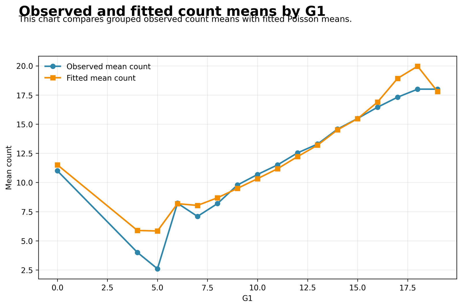
The fitted mean increases strongly across G2, while the observed data retain discrete bands and some low-score departures. The relationship is multiplicative on the mean scale.
β(G2) = 0.086381 and IRR = 1.090222. One additional G2 point corresponds to an estimated 9.02% increase in the conditional expected count.
The chart converts the log-rate coefficient into an outcome-scale pattern. G2 remains the dominant partial predictor after G1 and all demographic and study variables are included.
Check whether the observed pattern is approximately log-linear throughout the G2 range. Curvature at the edges would motivate polynomial or spline terms rather than a different dispersion statistic.
Python Chart 8: School-Level Observed and Fitted Counts
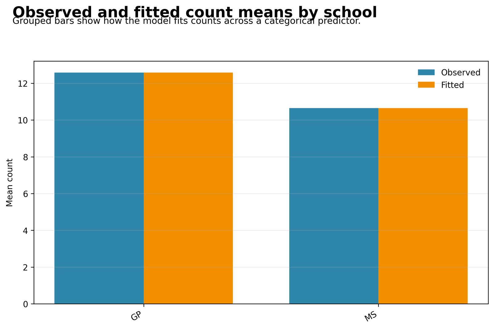
Raw school differences are reduced after the model adjusts for G1, G2, studytime, failures, absences, age, sex, and address.
The adjusted MS-versus-GP IRR is 0.967171, with ordinary 95% CI [0.916064, 1.021129] and p = 0.228159.
The factor coefficient compares conditional expected counts, not raw school means. Its ordinary interval includes one, so the unit-dispersion model does not support a nonzero adjusted school contrast at the 5% level.
Do not convert this fixed contrast into a causal school effect. Because students share schools, consider whether cluster-aware methods are required for the study design.
R Poisson Regression Charts and Explanations
The R charts reproduce the central distribution, calibration, Pearson-residual, and deviance-residual evidence. Python and R agree on the coefficients, null deviance, residual deviance, AIC, and Pearson dispersion when the formula, rows, factor references, and log link are aligned.
R Chart 1: Distribution of the Constructed Count
The bars remain concentrated on the 0–20 grade scale. That bounded measurement differs from an open-ended event process and provides a substantive explanation for underdispersion.
R Chart 2: Observed Counts Versus Conditional Means
Discrete outcome bands are compared with continuous conditional means. R and Python fitted values agree to rounding because the same formula, link, records, and references are used.
R Chart 3: Pearson Residual Pattern
The compressed spread yields Pearson chi-square 155.365855 and dispersion 0.243139. The result is underdispersion, and it directly challenges ordinary Poisson standard errors.
R Chart 4: Deviance Residual Distribution
The distribution is concentrated near zero but extends much farther on the negative side. Several zero-grade records are substantially overpredicted by the log-linked mean.
Poisson Regression Coefficient Interpretation
Poisson Regression coefficients are interpreted on two linked scales. β describes the change in log conditional mean; exp(β) describes the multiplicative change in the conditional expected count. The exponentiated value is usually easier to communicate, but it must retain the predictor’s unit and factor reference.
G2
G2 has β = 0.086381 and IRR = 1.090222. One additional G2 point is associated with a fitted count multiplied by 1.090222, or approximately 9.02% higher, holding G1, studytime, failures, absences, age, school, sex, and address fixed. Its ordinary interval is entirely above one.
G1
G1 has β = −0.002184 and IRR = 0.997818. Its 95% IRR interval, 0.980252 to 1.015699, includes one. The result is conditional on G2, so it should be described as little unique adjusted contribution rather than no overall relationship.
Failures
Failures has β = −0.040593 and IRR = 0.960220. Each additional failure corresponds to an estimated 3.98% lower fitted conditional count. The ordinary interval, 0.913453 to 1.009382, includes one, although Pearson-scaled inference is more precise because of underdispersion.
Absences
Absences has β = 0.002660 and IRR = 1.002663. One additional absence corresponds to approximately 0.266% higher fitted count. The ordinary interval includes one, and the effect is small per unit. No causal claim should be made from its adjusted sign.
School, Sex, and Address
School MS versus GP has IRR 0.967171, M versus F has 0.983359, and U versus R has 1.008429. Their ordinary intervals include one. These are conditional category contrasts, not raw group mean differences, random effects, or causal contextual impacts.
Intercept
The intercept IRR 4.832001 corresponds to all numeric predictors equal to zero and every factor at its reference category. That profile is not representative because zero age and prior grades are outside or at the edge of the meaningful design. The intercept is mainly an equation anchor.
Use the P-Value and Effect Size guides to keep statistical compatibility, interval precision, and substantive magnitude separate.
Poisson Regression Predictions and Worked Cases
Poisson Regression fitted values are conditional expectations and may contain decimals. The mean is calculated as μ̂ = exp(x′β). Raw residuals subtract the fitted mean from the observed count; Pearson residuals divide that discrepancy by √μ̂; deviance residuals measure signed likelihood discrepancy.
Representative case-level predictions and residuals
| Case | Observed | Fitted μ | Raw residual | Pearson residual | Deviance residual | Reason retained |
|---|---|---|---|---|---|---|
| 1 | 11 | 11.508059 | −0.508059 | −0.149766 | −0.150889 | Typical small error |
| 3 | 12 | 13.636190 | −1.636190 | −0.443085 | −0.452421 | Moderate overprediction |
| 62 | 16 | 10.312384 | +5.687616 | +1.771131 | +1.637239 | Largest positive residual |
| 164 | 0 | 8.456541 | −8.456541 | −2.908013 | −4.112552 | Most negative deviance residual |
| 173 | 1 | 9.763835 | −8.763835 | −2.804684 | −3.601430 | Largest negative raw residual |
| 587 | 0 | 8.400982 | −8.400982 | −2.898445 | −4.099020 | Extreme zero outcome |
| 640 | 0 | 7.803298 | −7.803298 | −2.793438 | −3.950519 | Extreme zero outcome |
| 649 | 11 | 10.590267 | +0.409733 | +0.125906 | +0.125107 | Small final-row error |
Case 62: largest positive residual
Case 62 has observed count 16 and fitted mean 10.312384, producing raw residual +5.687616, Pearson residual +1.771131, and deviance residual +1.637239. The model substantially underpredicts this case, but the standardized discrepancy is smaller than the most extreme negative residuals.
Case 164: most negative deviance residual
Case 164 has observed count 0 and fitted mean 8.456541. Its Pearson residual is −2.908013 and deviance residual is −4.112552. This record is especially incompatible with the fitted mean and contributes strongly to the negative residual tail.
Case 173: largest negative raw residual
Case 173 has observed count 1 and fitted mean 9.763835, giving raw residual −8.763835. It illustrates why calibration should be checked at the lower outcome boundary and why a bounded grade score may not follow an unrestricted Poisson probability process.
These are in-sample fitted values. Predictive performance on new students requires a holdout set, cross-validation, or another resampling design that respects grouping. Training RMSE and MAE should not be presented as external accuracy.
Poisson Regression Assumptions and Diagnostics
Core Assumptions
- Nonnegative count response on a meaningful observation unit
- Correct log-linked conditional mean
- Independent observations under the fitted likelihood
- Conditional variance approximately equal to μ
- Correct exposure offset when event opportunities differ
- Estimable predictors without exact linear dependence
Diagnostic Evidence Here
- All 649 rows are retained
- Null deviance falls from 745.6073 to 247.0655
- Pearson dispersion is only 0.243139
- Negative residual tail contains zero-grade cases
- Fitted means exceed the natural score ceiling
- School clustering is not represented by a correlation model
Outcome and Exposure
The response is nonnegative, but it is a bounded grade rather than an unlimited event count. No exposure offset appears. Therefore, rate-ratio language refers to multiplicative expected counts per student record, not verified incidence per unit time or opportunity.
Linearity on the Log Scale
The equation assumes linear log-mean effects for G1, G2, studytime, failures, absences, and age. Residual curvature or edge bias would support transformations, splines, polynomial terms, or interactions. Dispersion correction cannot fix an incorrect conditional mean.
Equidispersion
The ordinary model requires Var(Y|X)=μ. Pearson chi-square 155.365855 on 639 residual degrees of freedom gives 0.243139, so the assumption is not satisfied. This is underdispersion. The Quasi Poisson Regression guide shows how the same mean can be paired with scaled covariance.
Independence and Clustering
One row appears per student, but students share school contexts. Adding school as a fixed factor does not model within-school correlation. For cluster-aware population-average effects, compare Generalized Estimating Equations. For hierarchical effects, compare Multilevel Regression.
Collinearity
G1 and G2 share substantial information, making their partial coefficients sensitive to joint specification. Use Variance Inflation Factor and Tolerance Statistic as design diagnostics. Dispersion does not alter the predictor correlation structure.
Influence and Extreme Cases
Cases 164, 173, 587, 640, and 520 have large negative residuals, while case 62 has the largest positive residual. Use Cook’s Distance, Influence Diagnostics, and Outlier Detection to assess whether coefficient conclusions depend on individual observations.
Residual and Calibration Review
Read observed-versus-fitted, Pearson residual, and deviance residual plots together. Calibration evaluates the conditional mean, while dispersion evaluates the conditional variance. Review the complete Residual Analysis and Regression Diagnostics workflows before publication.
Poisson Regression in SPSS, Python, R and Excel
Python
Use statsmodels GLM with Poisson family and log link. Export coefficients, covariance, IRRs, likelihood measures, fitted means, Pearson residuals, deviance residuals, and the dispersion quotient.
- Primary chart source
- Transparent row-level prediction audit
- Check factor labels created by treatment coding
R
Use glm(..., family=poisson(link="log")). Relevel factors explicitly, calculate Pearson dispersion, and exponentiate coefficients with confidence intervals.
- Independent same-formula verification
- Convenient diagnostic residuals
- Compare coefficients after harmonizing labels
SPSS
Use GENLIN with Poisson distribution and log link. Declare categorical predictors and references, request goodness-of-fit and parameter estimates, and verify whether the scale is fixed or estimated.
- Menu and syntax workflow
- Review Pearson chi-square / df
- Do not assume default scale matches another program
Excel
Use the workbook to reproduce x′β, exp(x′β), rate ratios, residuals, dispersion, and selected confidence-interval arithmetic. Maximum-likelihood fitting and covariance should remain in statistical software.
- Useful teaching audit
- Transparent formula checking
- Retain full precision in calculation cells
The cross-software validation is performed once here. Python and R agree on n=649, residual df=639, null deviance=745.607271, residual deviance=247.065469, AIC=3009.799014, and dispersion=0.243139 when the model specification is aligned.
Poisson Regression Code
Python Poisson Regression workflow
import numpy as np
import pandas as pd
import statsmodels.api as sm
import statsmodels.formula.api as smf

df = pd.read_csv("dataset.csv")
df["count_outcome"] = df["G3"].round().clip(lower=0).astype(int)

formula = (
    "count_outcome ~ G1 + G2 + studytime + failures + "
    "absences + age + C(school) + C(sex) + C(address)"
)

model = smf.glm(
    formula=formula,
    data=df,
    family=sm.families.Poisson(link=sm.families.links.Log())
).fit()

result = pd.DataFrame({
    "beta": model.params,
    "standard_error": model.bse,
    "p_value": model.pvalues,
    "rate_ratio": np.exp(model.params),
    "rr_lower": np.exp(model.conf_int()[0]),
    "rr_upper": np.exp(model.conf_int()[1]),
})

df["fitted_mean"] = model.fittedvalues
df["raw_residual"] = model.resid_response
df["pearson_residual"] = model.resid_pearson
df["deviance_residual"] = model.resid_deviance

dispersion = model.pearson_chi2 / model.df_resid
print(model.summary())
print("Pearson dispersion:", dispersion)
print(result)
R Poisson Regression workflow
dat <- read.csv("dataset.csv", stringsAsFactors = FALSE)
dat$count_outcome <- as.integer(pmax(round(dat$G3), 0))

dat$school  <- relevel(factor(dat$school), ref = "GP")
dat$sex     <- relevel(factor(dat$sex), ref = "F")
dat$address <- relevel(factor(dat$address), ref = "R")

fit <- glm(
  count_outcome ~ G1 + G2 + studytime + failures +
    absences + age + school + sex + address,
  family = poisson(link = "log"),
  data = dat
)

pearson_chisq <- sum(residuals(fit, type = "pearson")^2)
dispersion <- pearson_chisq / df.residual(fit)

coefficient_table <- cbind(
  summary(fit)$coefficients,
  IRR = exp(coef(fit)),
  exp(confint.default(fit))
)

print(summary(fit))
print(dispersion)
print(coefficient_table)
SPSS GENLIN Poisson Regression syntax
GENLIN count_outcome BY school sex address
  WITH G1 G2 studytime failures absences age
  /MODEL school sex address G1 G2 studytime failures absences age
    INTERCEPT=YES
    DISTRIBUTION=POISSON
    LINK=LOG
  /CRITERIA CILEVEL=95
  /PRINT CPS DESCRIPTIVES MODELINFO FIT SUMMARY SOLUTION.
Confirm the actual SPSS reference categories and scale settings in the output before comparing coefficients, intervals, or Pearson statistics with Python and R.
Excel Poisson Regression audit formulas
Linear predictor for one row:
=Intercept + SUMPRODUCT(Coefficient_Range, Design_Row_Range)

Fitted conditional mean:
=EXP(Linear_Predictor)

Rate ratio:
=EXP(Coefficient)

Percentage change:
=(EXP(Coefficient)-1)*100

Raw residual:
=Observed_Count-Fitted_Mean

Pearson residual:
=(Observed_Count-Fitted_Mean)/SQRT(Fitted_Mean)

Pearson dispersion:
=SUMSQ(Pearson_Residual_Range)/Residual_Degrees_of_Freedom
26 Advanced Poisson Regression Topics
These panels extend Poisson Regression beyond the basic coefficient table into variance, measurement, dependence, prediction, influence, model selection, and reporting decisions.
1. Poisson Regression as a Conditional Mean Model
Poisson Regression models the expected count conditional on the predictors, not merely the marginal frequency distribution. The distinction matters because a poor unadjusted histogram can coexist with a useful conditional mean. In the worked equation, G2, G1, studytime, failures, absences, age, school, sex, and address jointly determine μ through the log link. Every coefficient interpretation is conditional on those terms.
2. Poisson Regression Equidispersion
The canonical probability model requires the conditional variance to equal the conditional mean. Equidispersion is not established by convergence, significant coefficients, or a lower deviance. The worked Pearson quotient is 0.243139, so the residual spread is much smaller than the unit-dispersion benchmark. This underdispersion is the central limitation of the ordinary variance and standard errors.
3. Why the Log Link Is Used
Poisson Regression uses log(μ)=Xβ so exponentiation guarantees positive fitted means. A coefficient is additive on the log scale and multiplicative on the count scale. The link does not constrain the fitted mean to the observed grade ceiling, which explains why the maximum fitted value, 21.9136, can exceed the observed maximum score.
4. Likelihood and Maximum-Likelihood Estimation
The ordinary model has a complete Poisson probability mass function, so it supports maximum-likelihood estimation, likelihood-based deviance, and AIC. The saved AIC is 3009.799014. That value can compare candidate Poisson likelihood models fitted to the same response and records, but it cannot prove that the preferred candidate satisfies equidispersion or measurement validity.
5. Null Deviance and Residual Deviance
Poisson Regression null deviance is 745.607271 and residual deviance is 247.065469. The reduction shows that the predictor set organizes the conditional mean much better than an intercept-only model. It does not demonstrate causal identification or validate the probability variance. Deviance fit and Pearson dispersion answer different questions and should be reported separately.
6. Rate Ratios Versus Additive Effects
Poisson Regression exponentiates β to obtain an incidence rate ratio. G2’s IRR of 1.090222 means a 9.02% multiplicative increase per point, holding the remaining design columns fixed. It does not mean an additive increase of 0.086 grades. Percentage changes are calculated as 100[exp(β)−1].
7. Rate Ratios Without an Exposure Offset
The term incidence rate ratio is conventional, but the worked model has no exposure denominator. Its coefficients compare expected counts per record, not events per person-year, area, or opportunity. Adding log exposure as an offset would change the scientific estimand and the fitted means; it requires a verified exposure variable.
8. Factor Reference Categories
Poisson Regression factor coefficients depend on reference coding. School compares MS with GP, sex compares M with F, and address compares U with R. Reversing the reference category would invert the displayed rate ratio but would not alter fitted means. Reports should name both the compared and reference levels.
9. G1 and G2 Collinearity
Poisson Regression includes two related prior grades. G1’s adjusted IRR is 0.997818 after G2 is held fixed, but this does not imply that G1 is unassociated with final performance in a simple analysis. It means G1 contributes little unique log-mean information beyond the later G2 measure and the remaining predictors.
10. Poisson Regression Underdispersion
Underdispersion can occur when outcomes are bounded, regulated, scheduled, or otherwise more regular than a Poisson process. Here the response is a score limited by the educational scale. The value 0.243139 is therefore substantively plausible. It should prompt variance correction and outcome-model reflection rather than being relabeled as overdispersion.
11. Quasi-Poisson Sensitivity Analysis
A Quasi Poisson Regression sensitivity analysis keeps the same β values and fitted means but multiplies covariance by φ. With φ below one, scaled standard errors become smaller. That comparison can reveal how ordinary unit-dispersion uncertainty affects decisions, but it does not create a new conditional relationship.
12. Negative Binomial Regression Is Not Automatic
Negative Binomial Regression is commonly used for variance greater than the mean, often through μ+αμ². The worked evidence points in the opposite direction. Choosing a negative-binomial model merely because the Poisson diagnostic failed would ignore the sign of the dispersion problem.
13. Bounded Counts and Alternative Outcome Models
The G3-derived response is integer-valued but also bounded and educational. Poisson Regression is mathematically convenient, yet an ordinary linear model, ordinal model, or another bounded-response approach may align more closely with the measurement process. Model choice should begin with what the outcome represents, not only with whether its values are integers.
14. Pearson Residuals
A Poisson Regression Pearson residual divides y−μ̂ by √μ̂. The sum of squared Pearson residuals is used to calculate dispersion. Plotting them against fitted values evaluates centering, curvature, and changing spread. The global quotient can be correct while subgroup-specific patterns reveal inadequacy.
15. Deviance Residuals
Poisson Regression deviance residuals express each observation’s signed contribution to the model-versus-saturated deviance. They are useful for identifying cases poorly represented by the fitted mean. The most negative value, −4.1126, occurs for a zero outcome fitted near 8.46. Such cases require investigation, not automatic exclusion.
16. Influence and Leverage
Poisson Regression influence depends on both residual size and leverage in the design matrix. A case with an unusual predictor profile can alter coefficients even when its residual is moderate. Generalized Cook’s distance, leverage, case-deletion changes, and DFBETAs should supplement residual inspection when influential observations are a concern.
17. Nonlinearity on the Log Scale
The worked Poisson Regression equation contains linear main effects. It assumes a constant log-rate change per unit of G1, G2, studytime, failures, absences, and age. Curvature in observed-versus-predictor plots requires polynomial terms, splines, categories, or another link—not a different dispersion label.
18. Interaction Terms
Poisson Regression interactions make one rate ratio conditional on another variable. A G2-by-school term would allow the G2 slope to differ between GP and MS. The current model assumes common slopes across categories. Interactions should be motivated before estimation and interpreted through combined coefficients or predicted means.
19. Zero Inflation
The presence of zero outcomes does not by itself prove a structural-zero process. Zero-Inflated Poisson Regression assumes a latent class that generates certain zeros in addition to Poisson sampling zeros. The grade file does not establish that mechanism. Model selection should rely on scientific plausibility, zero calibration, likelihood evidence, and positive-count diagnostics.
20. Clustered Observations
Poisson Regression treats residual contributions as independent. Students share schools, so including school as a fixed contrast adjusts average differences but does not model within-school correlation. With genuine clustering, use generalized estimating equations, cluster-robust covariance, or a multilevel count model suited to the number of clusters.
21. Robust Standard Errors
A sandwich covariance can protect Poisson Regression inference against broader variance misspecification while retaining the same mean coefficients. It differs from Pearson scaling because it does not impose one proportional multiplier. Robust covariance still requires appropriate independence or clustering assumptions and does not repair a misspecified mean.
22. Prediction and Conditional Means
Poisson Regression fitted values are expectations and may be non-integers. They should not be rounded before residuals or likelihood calculations. A future predictive distribution requires the full probability model; when equidispersion fails, ordinary Poisson prediction intervals can be misleading even if the mean estimate is useful.
23. In-Sample Versus Out-of-Sample Performance
The reported RMSE 1.4353 and MAE 0.9372 are calculated on the same 649 rows used for estimation. They describe training fit, not external prediction. A predictive claim requires a test set, cross-validation, or resampling that preserves any grouping structure.
24. Causal Interpretation
Poisson Regression coefficients in this observational grade analysis are conditional associations. Neither the log link nor maximum likelihood removes confounding, measurement error, selection, or reverse causation. Statements should use terms such as associated with, conditional mean, or adjusted ratio unless a causal design supports stronger language.
25. Reporting Precision and Reproducibility
Poisson Regression calculations should retain full precision while public tables use consistent rounding. Report n, residual degrees of freedom, coefficient, standard error, IRR, confidence interval, p-value, deviance, AIC, Pearson chi-square, and dispersion. The downloadable files preserve the detailed arithmetic without publishing 649 repetitive rows.
26. Choosing the Final Count Model
Poisson Regression should be retained only when its outcome interpretation, log mean, independence structure, and variance assumptions are acceptable for the research purpose. In this example, the mean equation is informative but equidispersion is not credible. The strongest conclusion is therefore a useful fitted mean accompanied by an explicit variance and measurement limitation.
APA-Style Poisson Regression Reporting
A complete report should identify how the outcome was created, the log link, sample size, predictor set, factor references, absence of an exposure offset, focal β values and IRRs, confidence intervals, p-values, deviance, AIC, Pearson chi-square, residual degrees of freedom, and dispersion conclusion.
Use association language rather than causal language. State that rate ratios describe expected counts per observation because no exposure offset is present. Do not hide the underdispersion result after presenting significant coefficients.
Poisson Regression Publication Checklist
Model and Data
- Define the count outcome and observation unit.
- State whether an exposure offset is used.
- List numeric predictors and factor references.
- Report n, parameters, and residual degrees of freedom.
- Show the log-linked mean and IRR formula.
- Explain why Poisson Regression is scientifically appropriate.
Results and Diagnostics
- Report β, SE, IRR, CI, and p for focal terms.
- Report null deviance, residual deviance, and AIC.
- Calculate Pearson chi-square / residual df.
- Label 0.243139 as underdispersion.
- Inspect residual, calibration, and influence plots.
- Discuss alternative variance and outcome models.
Poisson Regression Downloads
R Poisson Regression ReportIndependent GLM cross-check with the same formula, references, and dispersion calculation.
SPSS Poisson Regression OutputGENLIN tables retained as a separate software evidence source.
Worked Poisson Regression Excel WorkbookFitted-value, rate-ratio, residual, and dispersion arithmetic.
Poisson Regression Frequently Asked Questions
1. What is Poisson Regression?
Poisson Regression is a generalized linear model for a nonnegative count outcome. It uses a log link so predictors have multiplicative effects on the conditional expected count.
2. What question does Poisson Regression answer here?
It estimates how the expected G3-derived count changes with G1, G2, studytime, failures, absences, age, school, sex, and address while the other predictors are held fixed.
3. What does the G2 rate ratio mean?
The IRR of 1.090222 means that one additional G2 point multiplies the adjusted fitted count by about 1.090, corresponding to an estimated 9.02% increase.
4. Is G1 unrelated to the outcome?
No. Its near-null adjusted coefficient means it contributes little unique information after G2 and the remaining predictors are included. It is not a statement about the unadjusted G1 relationship.
5. Is the equidispersion assumption satisfied?
No. Pearson chi-square divided by 639 residual degrees of freedom is 0.243139, far below one. The result indicates strong underdispersion.
6. Is 0.243139 overdispersion?
No. Values above one indicate overdispersion; values below one indicate underdispersion. Calling this result overdispersion would reverse the evidence.
7. Why can a fitted count contain decimals?
A fitted value is the conditional expectation over possible counts. It is not required to be an observed integer for one student.
8. Does the model include an offset?
No. There is no exposure variable or log offset, so the rate ratios compare expected counts per record rather than rates per verified unit of time or opportunity.
9. Can AIC be reported?
Yes for the ordinary maximum-likelihood Poisson model. The saved AIC is 3009.799014. A true quasi-Poisson fit does not provide ordinary likelihood-based AIC.
10. Why is the fitted maximum above 20?
The log-linked mean is positive but unbounded. It does not know that the grade scale ends at 20, so fitted values can exceed the natural outcome ceiling.
11. Should Negative Binomial Regression replace this model?
Not automatically. Negative binomial regression is primarily designed for overdispersion, while this model is strongly underdispersed.
12. Should zero-inflated regression be used because some grades are zero?
Not without evidence of a separate structural-zero mechanism. A few zeros in a bounded grade distribution do not establish a latent always-zero class.
13. Which predictors are statistically significant in the ordinary model?
G2 is the clear supported slope under the ordinary unit-dispersion covariance. Most other 95% rate-ratio intervals include one.
14. Why do quasi-Poisson p-values differ?
Pearson scaling changes the covariance and standard errors while leaving the coefficients and rate ratios unchanged. With φ below one, scaled standard errors are smaller.
15. What should an APA-style report include?
Report the outcome construction, link, sample size, predictors and references, focal coefficients and IRRs, confidence intervals, deviance, AIC, Pearson chi-square, dispersion, and the underdispersion limitation.
16. What is the main conclusion?
The model captures a strong G2-related conditional mean pattern and substantially reduces deviance, but ordinary Poisson equidispersion is not credible for this bounded grade response.
Poisson Regression Conclusion
The worked Poisson Regression model provides a clear multiplicative conditional mean for the 649-case G3-derived count. It reduces deviance from 745.607271 to 247.065469, has AIC 3009.799014, and identifies G2 as the dominant positive adjusted predictor with IRR 1.090222 per point.
The distributional limitation is equally important. Pearson chi-square 155.365855 on 639 residual degrees of freedom gives dispersion 0.243139, showing strong underdispersion. The ordinary probability model expects substantially more residual variation than appears in the bounded grade response. Therefore, ordinary model-based standard errors and prediction statements should not be treated as fully validated.
The defensible conclusion is dual: the log-linked mean captures useful grade progression, while equidispersion is not credible. A final report should preserve the ordinary likelihood fit and rate-ratio interpretation, disclose the bounded outcome and absent offset, examine extreme residuals and clustering, and compare a variance-adjusted or alternative outcome model.
Continue with Quasi Poisson Regression for the direct dispersion sensitivity analysis, Negative Binomial Regression for likelihood-based overdispersion comparisons, and Generalized Estimating Equations when correlated observations are central.

