
Probit Regression: Formula, Interpretation, Python, R, SPSS and Excel Guide
Probit Regression models a binary outcome by connecting a linear predictor to probability through the standard normal cumulative distribution function. This worked analysis predicts whether G3 is at least 10 from earlier grades, study behavior, attendance, age, school, sex, and address.
549 pass outcomes
McFadden pseudo-R² 0.6800
Accuracy 93.84%
Probit Regression Model Overview
Probit Regression is a generalized linear modeling method for an outcome coded with two categories, usually 0 and 1. Instead of predicting the observed binary value with an unrestricted straight line, Probit Regression estimates a latent linear score and converts that score into a valid probability through the standard normal cumulative distribution function.
Definition of Probit Regression
Probit Regression is a binary-response model in which the probability of an event is written as Φ(Xβ), where Φ is the cumulative distribution function of a standard normal random variable. The model ensures that every fitted probability remains between 0 and 1 while allowing several continuous and categorical predictors to contribute to the event probability.
The term probit is historically associated with a probability unit derived from the inverse normal distribution. In modern regression practice, the important idea is that the inverse standard normal CDF transforms a probability into a linear predictor. The fitted equation therefore operates on a latent z-score scale, while interpretation for readers is usually returned to predicted probabilities and marginal effects.
What Question Does Probit Regression Answer?
Probit Regression answers how a collection of predictors changes the probability that an observation belongs to category 1 rather than category 0. In the present worked analysis, category 1 means that final grade G3 is at least 10, while category 0 means G3 is below 10. The model asks how G1, G2, studytime, failures, absences, age, school, sex, and address jointly relate to that pass probability.
The method can also answer classification questions after a probability cutoff is chosen. A cutoff of 0.50 is used here: fitted probabilities at or above 0.50 are classified as 1, and lower probabilities are classified as 0. Classification is a secondary decision layer. The primary statistical output remains the modeled probability.
When Probit Regression Is Used
Probit Regression is used when the dependent variable is binary and a latent normally distributed propensity is substantively plausible or conventionally preferred. It is common in economics, policy analysis, education research, toxicology, credit-risk modeling, adoption studies, labor-market analysis, and any setting where an unobserved continuous tendency is believed to cross a threshold that produces an observed yes/no result.
Examples include employed versus unemployed, approved versus rejected, adopted versus not adopted, disease present versus absent, purchase versus no purchase, and pass versus fail. The model is especially natural when the binary result is interpreted as a thresholded version of an underlying continuous process.
Core Probit Regression Formula
The linear predictor is commonly written as η = Xβ. The probit link connects the probability to that predictor:
The fitted probability is then recovered with the standard normal CDF:
At η = 0, the fitted probability is 0.50 because Φ(0) = 0.50. Positive latent scores produce probabilities above 0.50, while negative latent scores produce probabilities below 0.50.
Latent-Variable Interpretation
Probit Regression can be represented with an unobserved continuous variable Y*. The observed outcome equals 1 when Y* crosses a threshold and equals 0 otherwise:
This latent-variable formulation explains why coefficients use a standard-normal z scale. A positive coefficient raises the latent propensity and therefore raises the probability of category 1, holding other predictors constant. A negative coefficient lowers that propensity and probability.
Probit Regression Versus Logistic Regression
Logistic Regression uses the logistic CDF, while Probit Regression uses the standard normal CDF. Both produce S-shaped probability curves, valid probabilities, and usually similar classifications. Logistic coefficients are naturally converted to odds ratios. Probit coefficients are naturally interpreted on a latent normal scale and through marginal probability effects.
The logistic distribution has slightly heavier tails than the normal distribution. Consequently, coefficient magnitudes differ even when fitted probabilities are similar. A rough comparison sometimes rescales logit coefficients, but exact interpretation should use each model’s own predicted probabilities rather than treating the coefficients as interchangeable.
Is Probit Regression a Generalized Linear Model?
Yes. Probit Regression is a binomial Generalized Linear Model with a probit link. The random component is binomial, the systematic component is the linear predictor Xβ, and the link function is Φ⁻¹(p). Maximum likelihood estimation is used rather than ordinary least squares.
How Probit Coefficients Are Interpreted
A coefficient describes the change in the latent probit index for a one-unit predictor increase, holding the other variables fixed. It does not describe one constant percentage-point change in probability. The probability effect depends on the current value of η because the standard normal density is highest near η = 0 and becomes small in the tails.
Here φ is the standard normal probability density function. The same coefficient can create a large probability change for a case near p = 0.50 and a very small change for a case already near p = 0 or p = 1.
Marginal Effects and Discrete Changes
For a continuous predictor, the marginal effect is φ(η)β. For a binary predictor, a discrete change is usually clearer: calculate the predicted probability once with the indicator equal to 0 and again with it equal to 1 while keeping the remaining variables fixed. Average marginal effects repeat this calculation or derivative across observations and average the results.
At η = 0 in this worked model, the instantaneous G2 marginal effect is approximately 0.319 probability points per one-unit increase because φ(0) × 0.8003 ≈ 0.3193. This is a marginal effect at the center of the probability curve, not an average effect for the whole sample.
Outcome Coding and Reference Categories
The event definition must be explicit because reversing 0 and 1 reverses coefficient signs and changes interpretation. Here probit_pass = 1 when G3 ≥ 10 and 0 otherwise. The reference groups are school GP, sex F, and address R. Indicator coefficients compare school MS with GP, male with female, and urban address U with rural address R.
Core Assumptions
- The outcome has two mutually exclusive categories coded consistently.
- Observations are independent unless clustering is modeled explicitly.
- The linear predictor is correctly specified on the probit scale.
- Continuous predictors have an appropriate functional form.
- Predictors do not exhibit perfect multicollinearity.
- Complete or quasi-complete separation does not prevent stable estimation.
- The sample contains enough events and non-events for the fitted parameters.
- Influential observations do not determine the fitted probability curve.
Advantages
- Produces fitted probabilities constrained to the 0–1 interval.
- Provides a direct latent-normal interpretation for threshold processes.
- Handles continuous and categorical predictors in one model.
- Supports probability predictions, marginal effects, classification, and scenario analysis.
- Is available in Python, R, SPSS, Stata, SAS, and Excel-based calculators.
- Often yields conclusions similar to logistic regression while offering a different theoretical link.
Limitations
- Raw coefficients are not percentage-point effects.
- Results can be sensitive to separation, rare outcomes, and influential cases.
- A 0.50 classification cutoff may be unsuitable for an imbalanced outcome or unequal error costs.
- Pseudo-R² does not have the same meaning as ordinary least-squares R².
- A good in-sample classification rate can overstate future performance without validation.
- The latent normal assumption may not be the best link for every application.
Current Worked Scenario
The analysis uses 649 observations from the student-performance data. The binary outcome equals 1 for the 549 students with G3 ≥ 10 and 0 for the 100 students with G3 below 10. The event rate is therefore 84.59%.
Predictors are G1, G2, studytime, failures, absences, age, school, sex, and address. The fitted model has log likelihood −89.2387, null log likelihood −278.8928, likelihood-ratio χ²(9) = 379.3081, p < .001, AIC = 198.4774, and McFadden pseudo-R² = 0.6800.
Using a 0.50 cutoff, the model correctly classifies 609 of 649 cases, for accuracy of 93.84%. It identifies 532 of 549 events and 77 of 100 non-events. G2 is the strongest positive coefficient, B = 0.8003, while school MS has a statistically significant negative coefficient, B = −0.5888.
Quick Answer
Model-fit result
- Log likelihood: −89.2387
- Null log likelihood: −278.8928
- Likelihood-ratio χ²(9): 379.3081
- AIC: 198.4774
- Log loss: 0.1375
Classification result
- True negatives: 77
- False positives: 23
- False negatives: 17
- True positives: 532
- Sensitivity: 96.90%
- Specificity: 77.00%
Table of Contents
- Why this analysis needs Probit Regression
- How Probit Regression works
- Variables used and coding
- Model fit and classification results
- Eight Python chart stories
- Eight R charts and explanations
- Coefficient and marginal-effect interpretation
- Predictions, classification, and cutoff choice
- Assumptions and diagnostics
- Python, R, SPSS, and Excel workflows
- Code
- Advanced Probit Regression topics
- APA-style reporting
- Publication checklist
- Downloads and chart resources
- Related Salar Cafe guides
- Frequently asked questions
Why This Analysis Needs Probit Regression
An ordinary linear probability model could regress the 0/1 outcome directly on the predictors, but it can generate fitted values below 0 or above 1 and assumes one constant probability effect across all covariate patterns. Probit Regression replaces that straight probability line with a smooth S-shaped relationship.
The event is common rather than rare: 549 of 649 observations are coded 1. A model that always predicts the majority class would already achieve 84.59% accuracy. Probit Regression must therefore be evaluated against that baseline rather than praised solely for a high raw accuracy figure.
The fitted classification accuracy is 93.84%, an improvement of approximately 9.25 percentage points over the majority-class rule. More importantly, the model produces individual probabilities, identifies 77% of non-events, and achieves 96.90% sensitivity for events.
G1 and G2 are continuous grade measures. Their relationship with event probability is naturally nonlinear even when they enter the latent index linearly. A one-unit grade increase changes probability most for observations near the decision boundary and less for observations already assigned an extreme probability.
How Probit Regression Works
Combine the intercept, continuous predictors, and indicator variables into η = Xβ.
Apply the standard normal CDF so p̂ = Φ(η) remains between 0 and 1.
Compare p̂ with a declared cutoff such as 0.50, then evaluate the resulting errors.
Maximum likelihood chooses coefficients that make the observed pattern of zeros and ones most probable under the fitted model. Unlike least squares, the method does not minimize ordinary squared residuals. The log likelihood, deviance, AIC, and likelihood-ratio test are therefore central fit measures.
The standard normal CDF is monotonic. Any predictor with a positive coefficient raises probability for every case, although the size of the probability increase varies. Any predictor with a negative coefficient lowers probability for every case, again with a context-dependent magnitude.
At the 0.50 cutoff, η = 0 is the class boundary. Raising the cutoff above 0.50 demands stronger evidence before assigning class 1 and usually increases specificity while reducing sensitivity. Lowering it usually does the opposite.
Variables Used and Coding
| Variable | Role | Definition or coding | Model interpretation |
|---|---|---|---|
| probit_pass | Binary outcome | 1 when G3 ≥ 10; 0 when G3 < 10 | Probability modeled by Probit Regression |
| G1 | Continuous predictor | First-period grade | Earlier academic performance |
| G2 | Continuous predictor | Second-period grade | Main academic predictor |
| studytime | Ordered numeric predictor | Weekly study-time category | Conditional change in latent pass propensity |
| failures | Count predictor | Number of prior class failures | Academic difficulty history |
| absences | Count predictor | Recorded absences | Attendance-related predictor |
| age | Continuous predictor | Age in years | Conditional demographic association |
| school_MS_dummy | Binary indicator | 1 = MS; 0 = GP | MS compared with reference school GP |
| sex_M_dummy | Binary indicator | 1 = male; 0 = female | Male compared with reference female |
| address_U_dummy | Binary indicator | 1 = urban; 0 = rural | Urban compared with reference rural address |
Model Fit and Classification Results
| Measure | Result | Interpretation |
|---|---|---|
| Sample size | 649 | All observations used in the fitted analysis |
| Number of fitted slopes | 9 | Six numeric predictors and three indicator contrasts |
| Log likelihood | −89.238714 | Maximized log likelihood of the fitted model |
| Null log likelihood | −278.892770 | Intercept-only comparison model |
| Likelihood-ratio χ² | 379.308112, df = 9, p < .001 | Predictors jointly improve fit over the null model |
| AIC | 198.477428 | Fit measure penalized for parameter count; useful for comparing candidate models |
| McFadden pseudo-R² | 0.680025 | Large improvement in log likelihood relative to the null model; not ordinary R² |
| Mean predicted probability | 0.845070 | Closely matches the observed event rate |
| Observed event rate | 0.845917 | 549 events among 649 observations |
| Log loss | 0.137502 | Probability scoring rule that penalizes confident wrong predictions |
609 correct of 649
532 of 549 events detected
77 of 100 non-events detected
532 of 555 predicted events correct
77 of 94 predicted non-events correct
Balance of event precision and sensitivity
McFadden pseudo-R² should not be described as “68% of variance explained.” It compares the fitted and null log likelihoods. For probability prediction, log loss, calibration, discrimination, and out-of-sample validation provide complementary information.
Worked Analysis Resources
The supplied reports and workbook contain model output, coefficient estimates, probability calculations, charts, and a transparent prediction calculator.
R Report PDFComplete R analysis, tables, and chart sequence
Eight Python Chart Stories
The supplied Python figures are explained with the observed pattern, exact model values, practical interpretation, and the diagnostic reason each chart matters for Probit Regression.
Chart 1: Binary Outcome Distribution
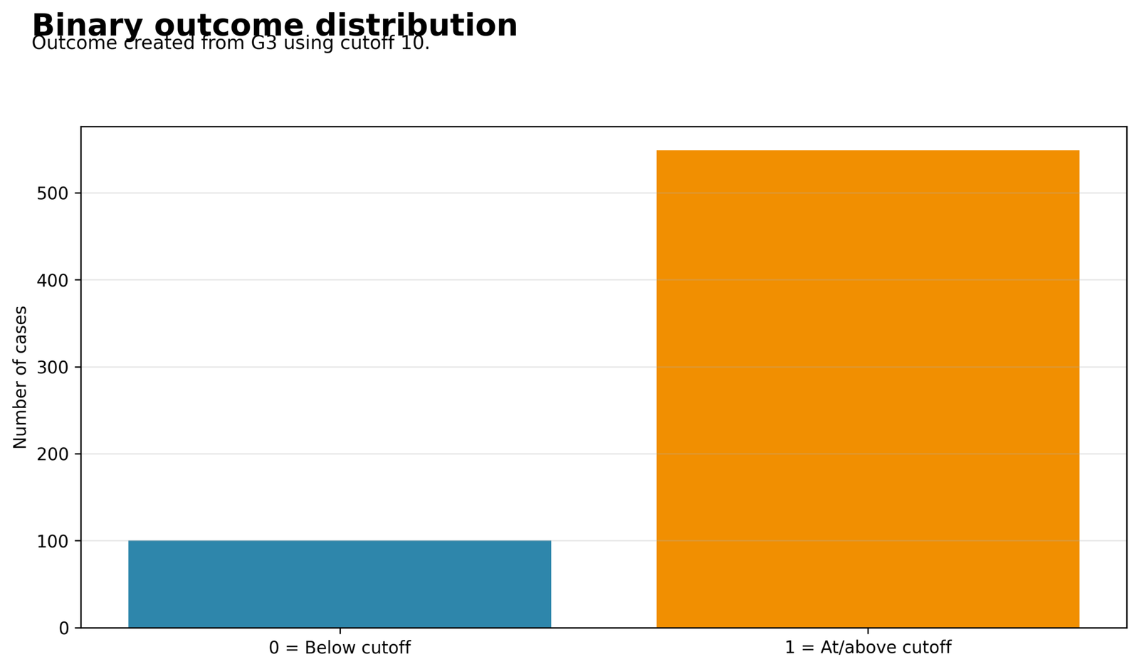
The event category is much larger than the non-event category. Most observations meet or exceed the G3 cutoff, so the response is imbalanced toward class 1.
There are 549 events and 100 non-events among 649 observations. The observed event rate is 84.59%, and the non-event rate is 15.41%.
The model predicts a common event rather than a rare one. Raw accuracy must be compared with a majority-class baseline of 84.59%, because predicting every case as 1 would already appear superficially successful.
Outcome balance affects cutoff choice, interpretation of accuracy, positive and negative predictive values, and the practical cost of false positives and false negatives.
Chart 2: Predicted Probability Distribution
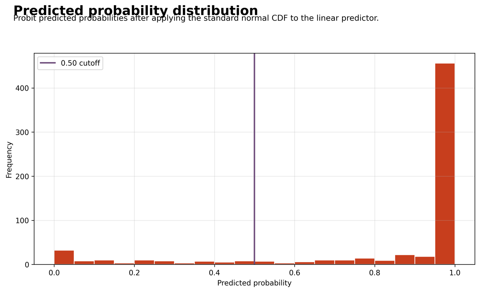
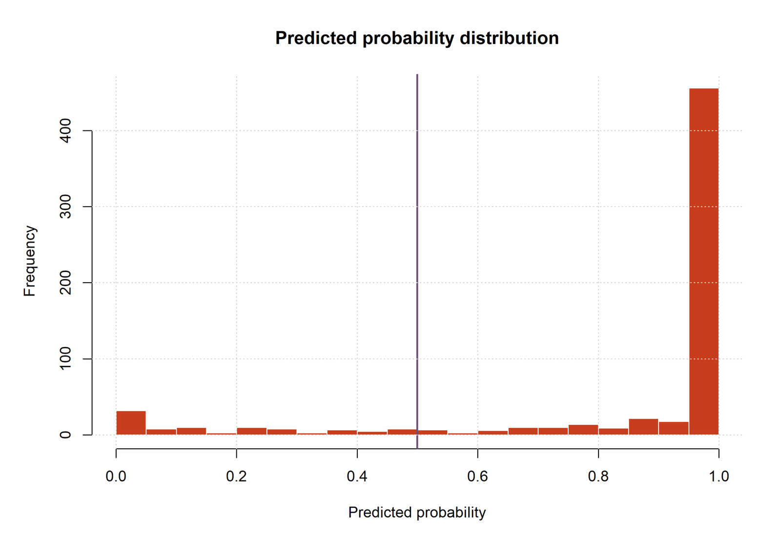
A very large concentration appears near probability 1.00, while a smaller concentration appears close to 0.00. Fewer cases occupy the middle of the probability scale, indicating substantial separation between many pass and non-pass observations.
The mean fitted probability is 0.845070, almost identical to the observed event rate of 0.845917. The vertical line at 0.50 marks the classification cutoff.
Most observations receive decisive predictions, especially event cases with high G1 and G2. The smaller set near the cutoff represents cases for which classification is more uncertain and more sensitive to the chosen threshold.
A probability histogram reveals confidence, polarization, and potential overconfidence that a single accuracy statistic cannot show. Extreme fitted probabilities also make log loss useful because it heavily penalizes confident errors.
Chart 3: Observed Class Versus Predicted Probability
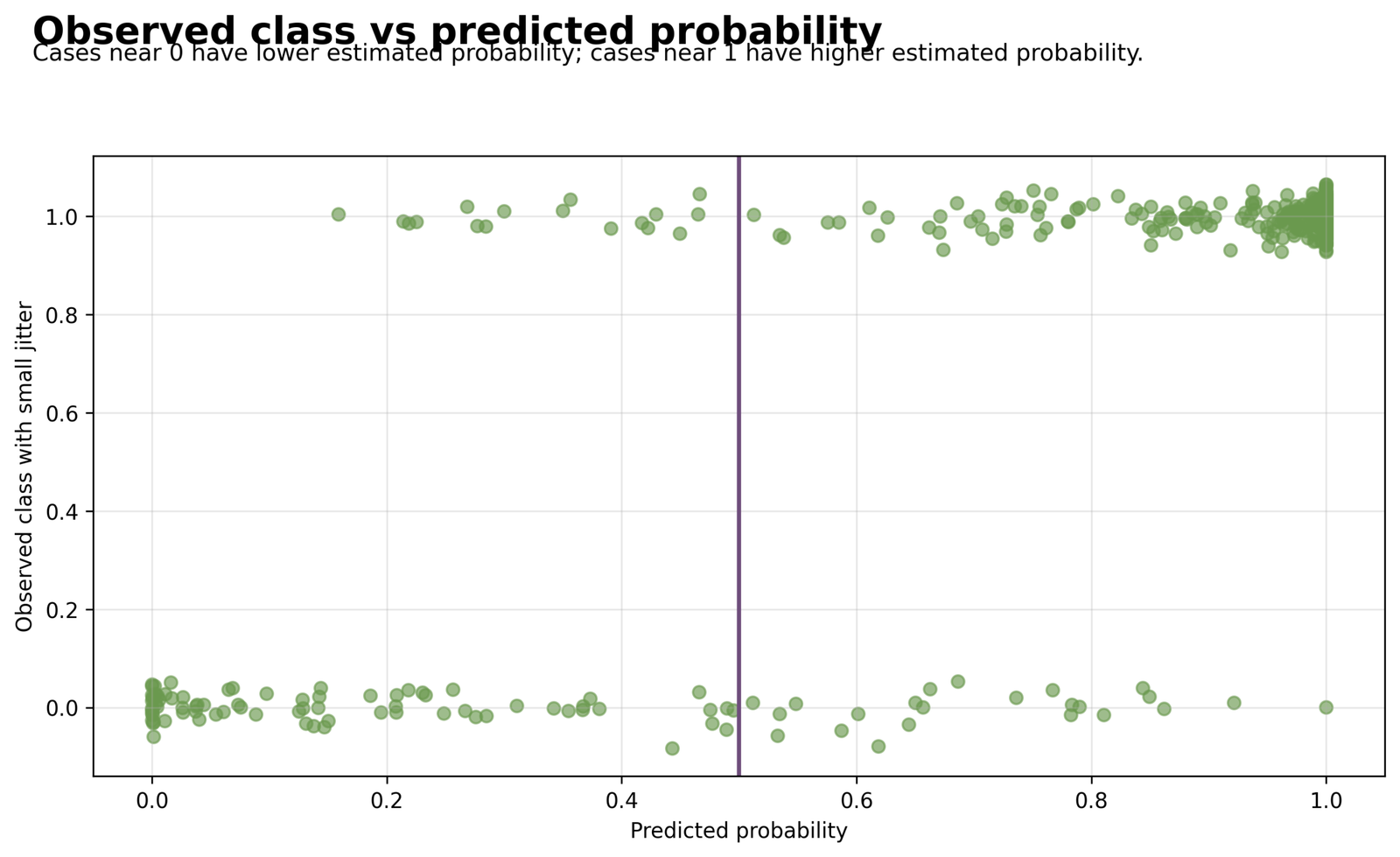
Most observed class-1 cases cluster at high fitted probabilities, while many class-0 cases cluster at low probabilities. Overlap remains around and above the 0.50 line, including some non-events assigned high probabilities and some events assigned low probabilities.
At the 0.50 cutoff, 532 events and 77 non-events are correctly classified. There are 17 false negatives and 23 false positives.
The fitted model separates the outcome groups strongly but not perfectly. False positives are non-pass observations whose earlier grades and covariates resemble pass cases. False negatives are pass observations that resemble the modeled non-pass profile.
This graph keeps probability information visible instead of reducing every case immediately to a class label. It identifies uncertain observations and confident mistakes that deserve diagnostic review.
Chart 4: Probability Residuals Versus Fitted Probabilities
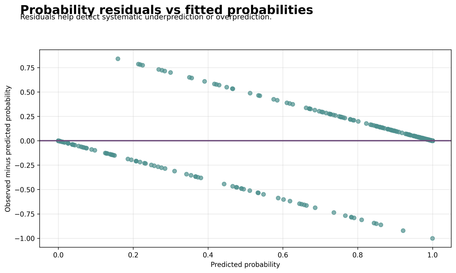
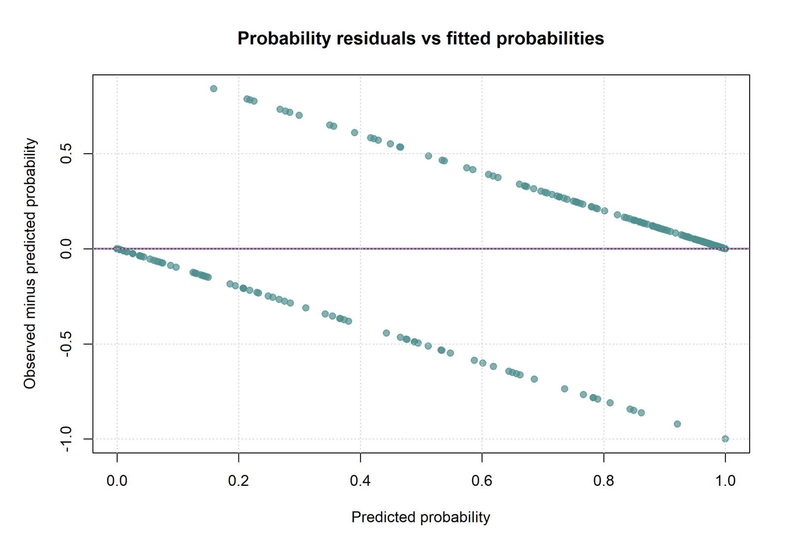
Two diagonal branches appear by construction. For observed events, residual = 1 − p̂ and lies above zero. For observed non-events, residual = −p̂ and lies below zero. Most points approach zero because many fitted probabilities are close to their observed class.
Residuals range approximately from −1.00 to +0.85. A non-event predicted near 1 produces a residual near −1, while an event predicted near 0.15 produces a residual near +0.85.
Large positive residuals are underpredicted events, and large negative residuals are overpredicted non-events. The extreme residuals correspond to the most consequential classification errors and may reflect unusual covariate combinations.
Raw residuals are intuitive but heteroskedastic for binary data. Pearson, deviance, leverage, and influence diagnostics should supplement this plot before drawing conclusions about model adequacy.
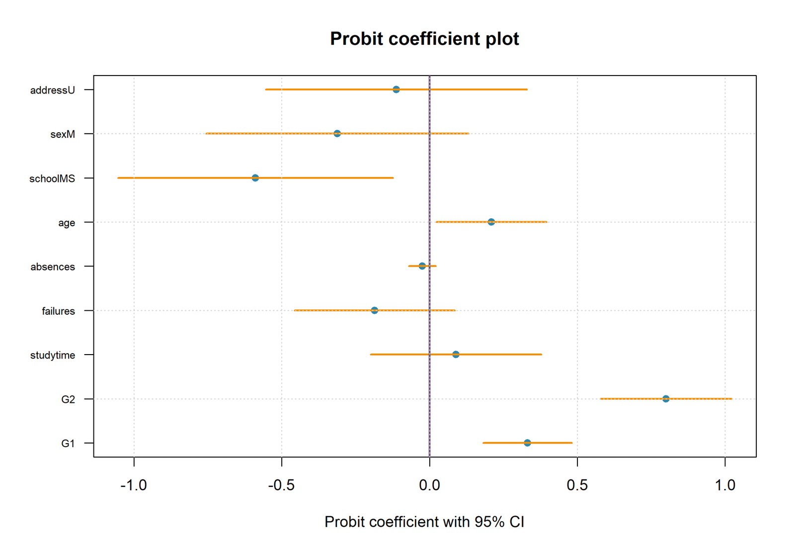
Chart 5: Probit Coefficients with 95% Confidence Intervals
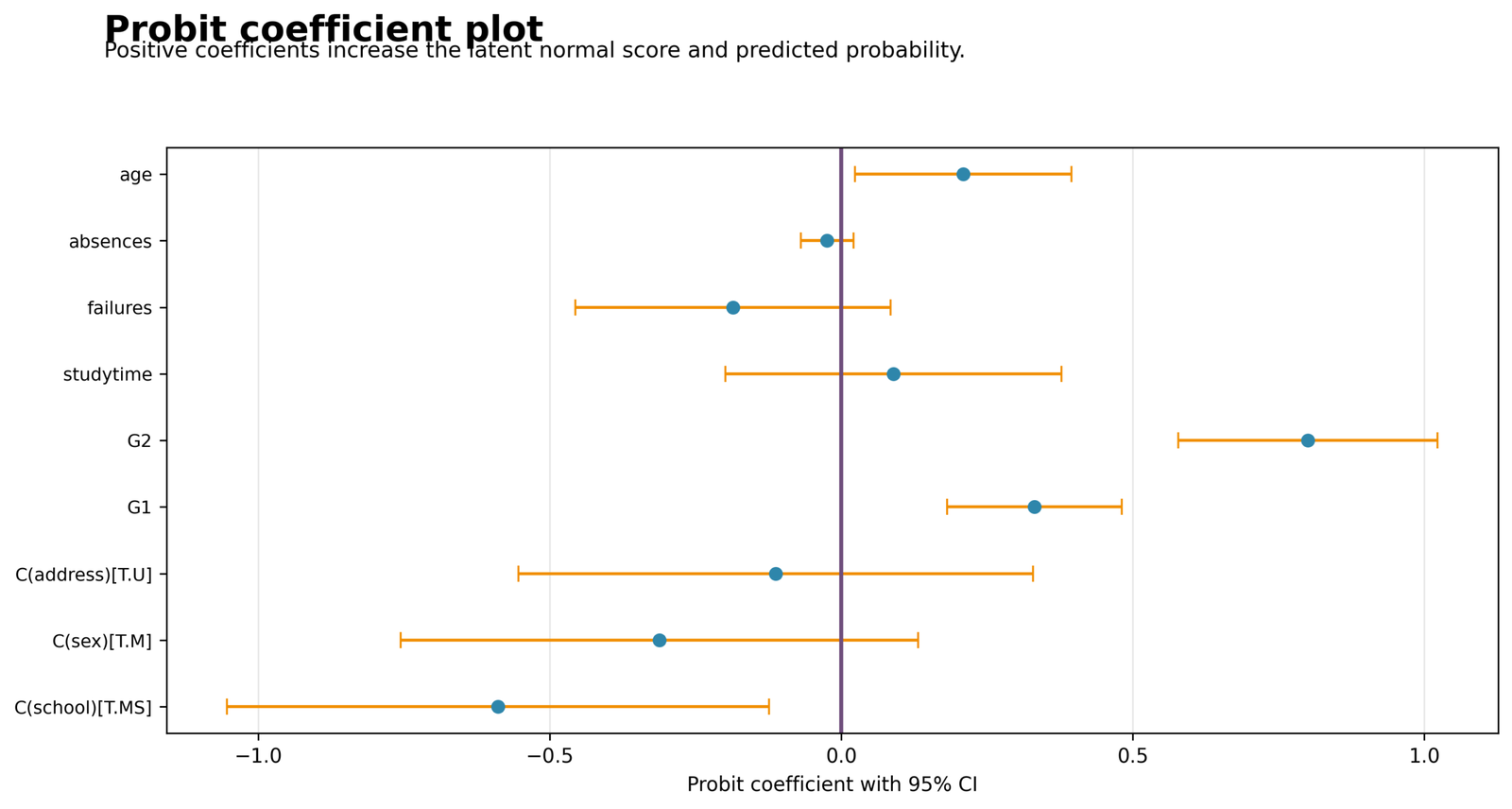
G2 is the largest positive coefficient, followed by G1 and age. School MS is the clearest negative categorical contrast. Confidence intervals for sex, address, studytime, failures, and absences cross zero.
G2 B = 0.800302, p < .001; G1 B = 0.331065, p < .001; age B = 0.209143, p = .0274; school MS B = −0.588822, p = .0131.
Holding the other variables fixed, higher G2, higher G1, and age shift the latent pass propensity upward. Attendance at school MS shifts it downward relative to school GP. Coefficient length does not equal a direct percentage-point effect.
The plot summarizes sign, uncertainty, and comparative latent-scale magnitude. Probability scenarios or marginal effects are still required for practical interpretation.
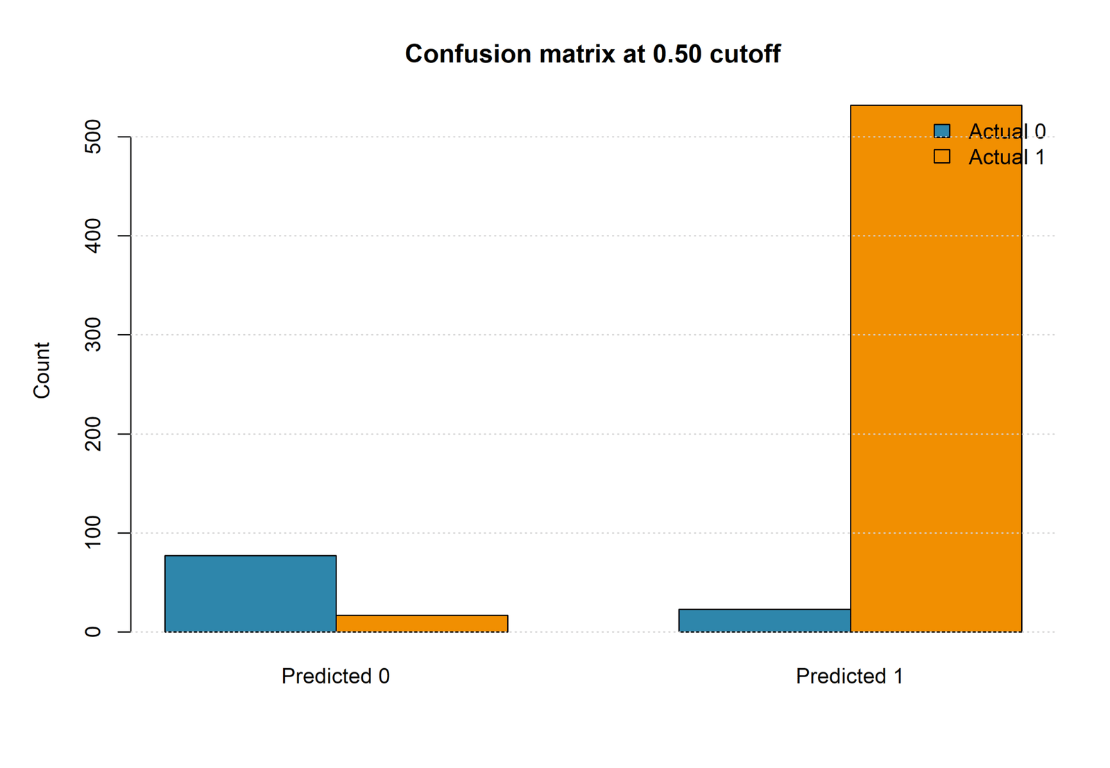
Chart 6: Confusion Matrix at the 0.50 Cutoff
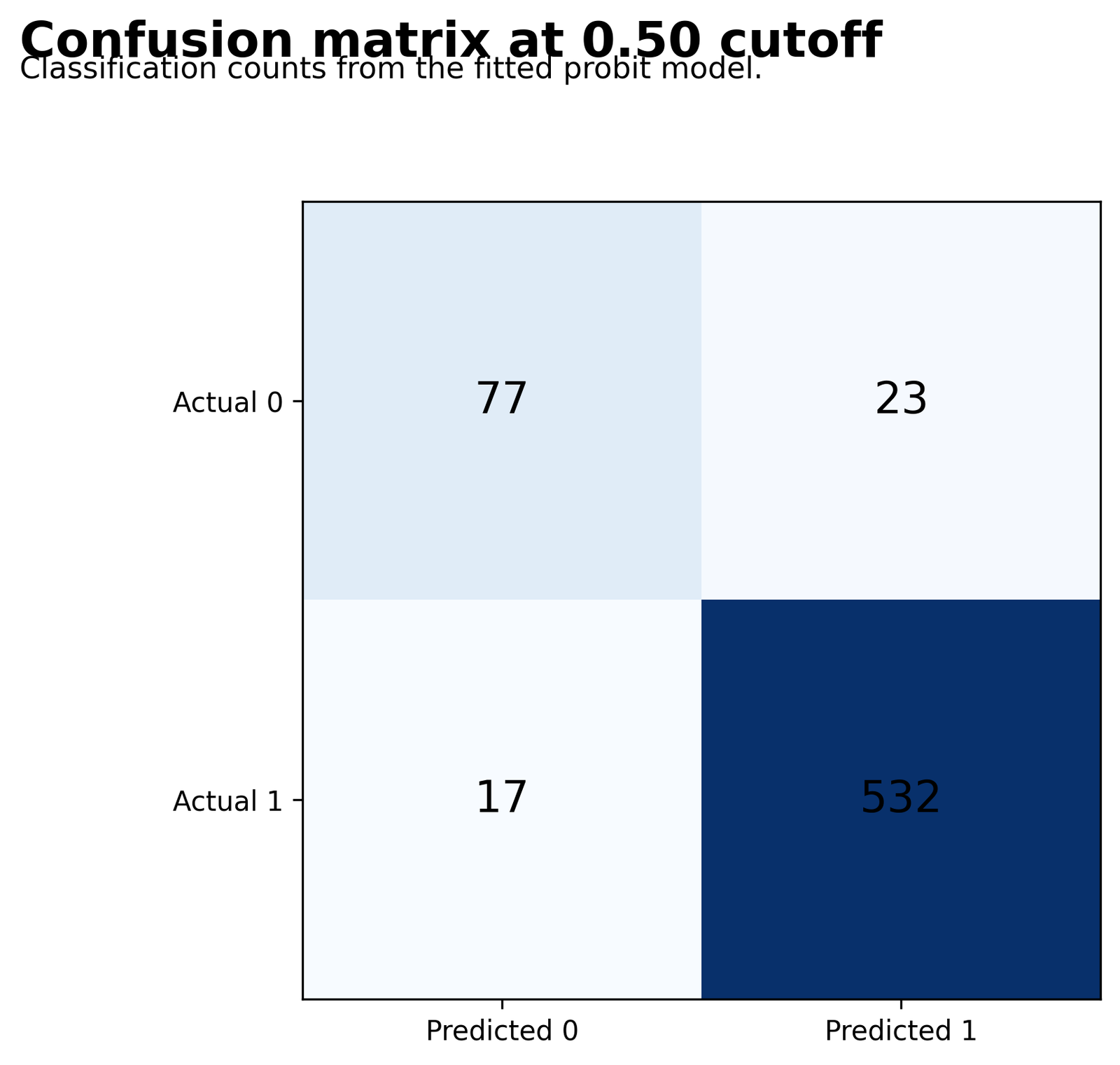
The largest cell is true positives because pass outcomes dominate the sample and are predicted very accurately. True negatives are also more common than false positives, but non-event classification is visibly weaker than event classification.
TN = 77, FP = 23, FN = 17, and TP = 532. Accuracy = 93.84%, sensitivity = 96.90%, specificity = 77.00%, and balanced accuracy = 86.95%.
The 0.50 threshold favors strong detection of pass outcomes while accepting more false positives than false negatives. Whether this balance is desirable depends on the practical consequences of each error type.
Accuracy alone hides asymmetric performance. The confusion matrix makes clear that the model is substantially better at identifying events than non-events.
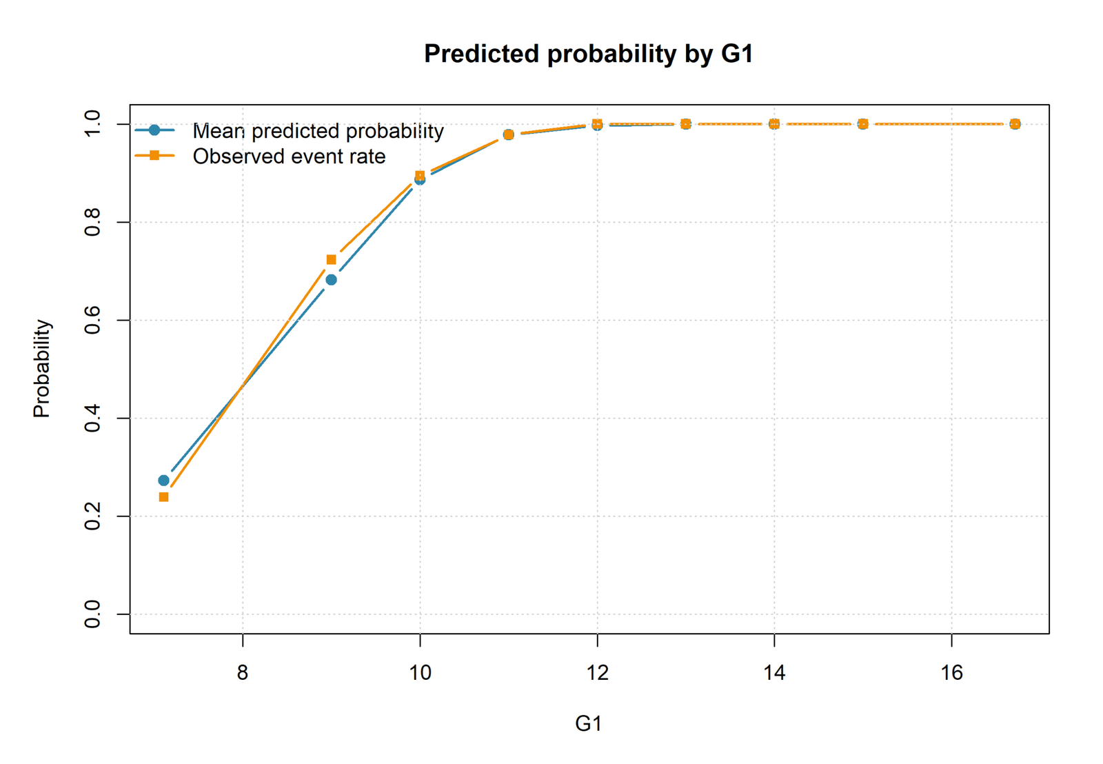
Chart 7: Predicted Probability by G1
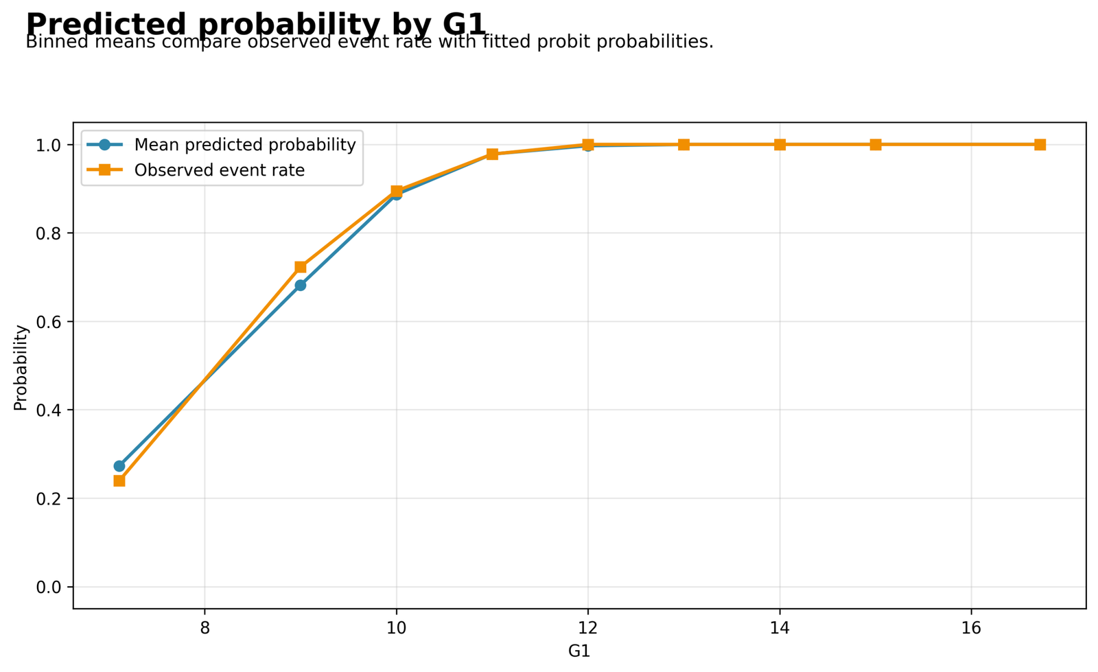
Both fitted and observed probabilities rise sharply from low G1 values and approach 1.00 around G1 = 12. The two lines remain close across the plotted bins, with only small discrepancies at the lower values.
At G1 near 7, the mean predicted probability is approximately 0.27 and the observed event rate about 0.24. Near G1 = 9 they are roughly 0.68 and 0.72; near G1 = 10 both are approximately 0.89; from G1 = 12 upward both are near 1.00.
G1 is strongly associated with pass probability, but the probability-scale relationship is nonlinear and saturates near 1.00. A one-point G1 increase matters more in the transition region than in the upper tail.
The close agreement of binned fitted and observed rates provides a useful visual calibration check for the main predictor, although full calibration assessment should use held-out data when possible.
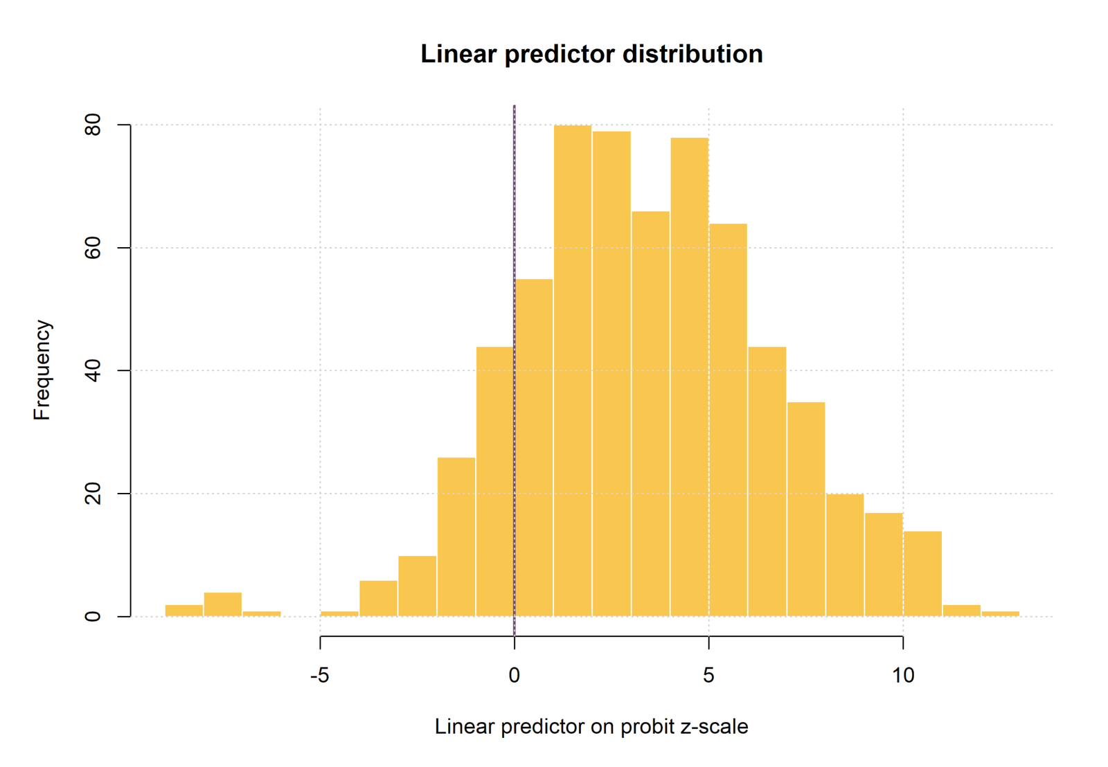
Chart 8: Linear Predictor Distribution
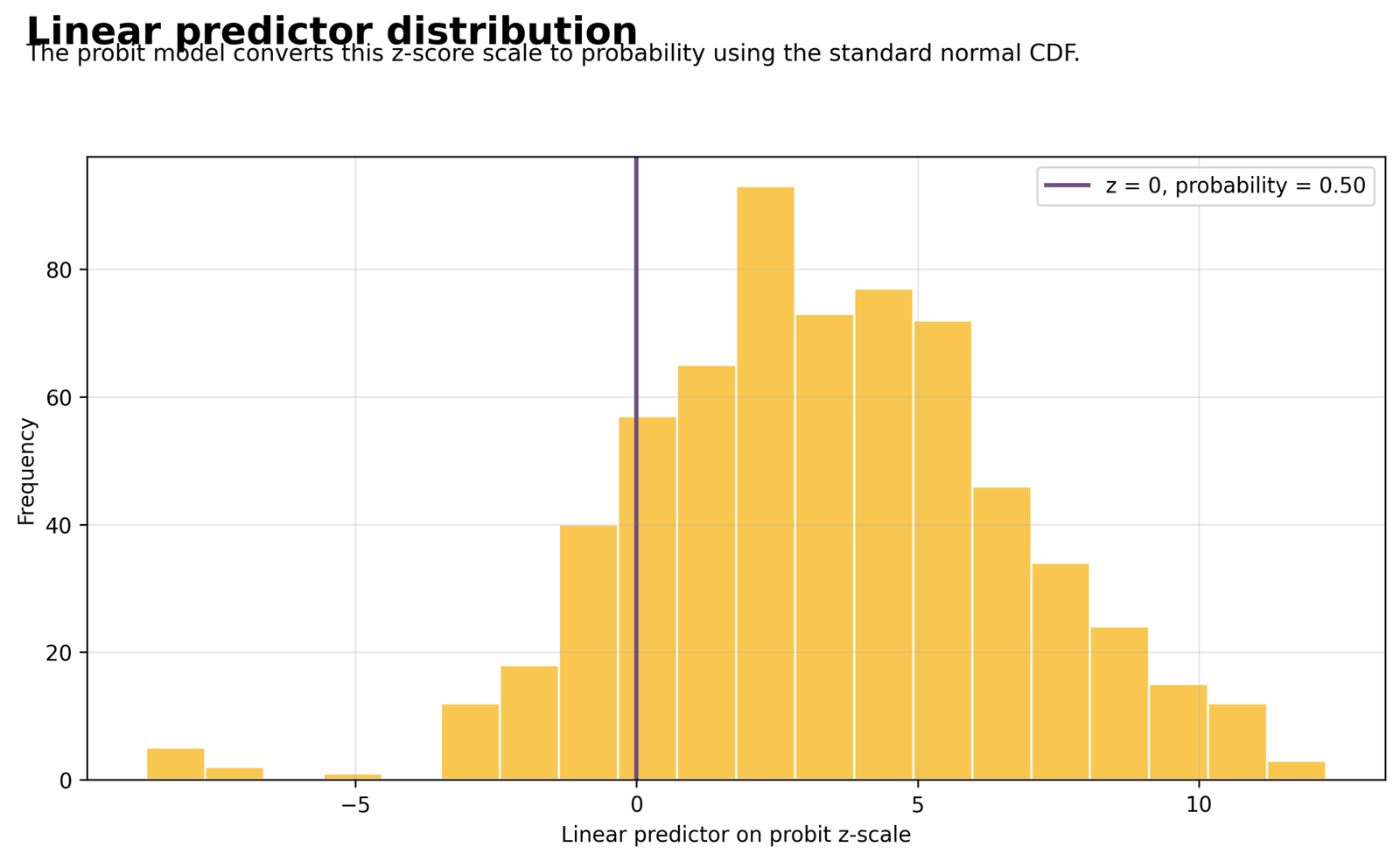
Most latent scores are positive, with the distribution concentrated roughly between 0 and 8 and a smaller negative tail. The vertical line at η = 0 marks the probability 0.50 boundary.
The visible latent-index range extends approximately from −8 to +12. Scores above zero produce predicted probabilities above 0.50; scores below zero produce probabilities below 0.50.
The strongly positive center reflects the high observed pass rate. Scores far into either tail are converted to probabilities extremely close to 1 or 0, explaining the polarized probability histogram.
This chart links coefficients to probabilities. It shows where cases fall on the latent scale and why equal changes in η do not create equal probability changes in the center and tails.
R Charts and Explanations
The R chart sequence reproduces the eight Probit Regression diagnostics with the same 649 observations, event coding, coefficient estimates, and 0.50 classification cutoff.
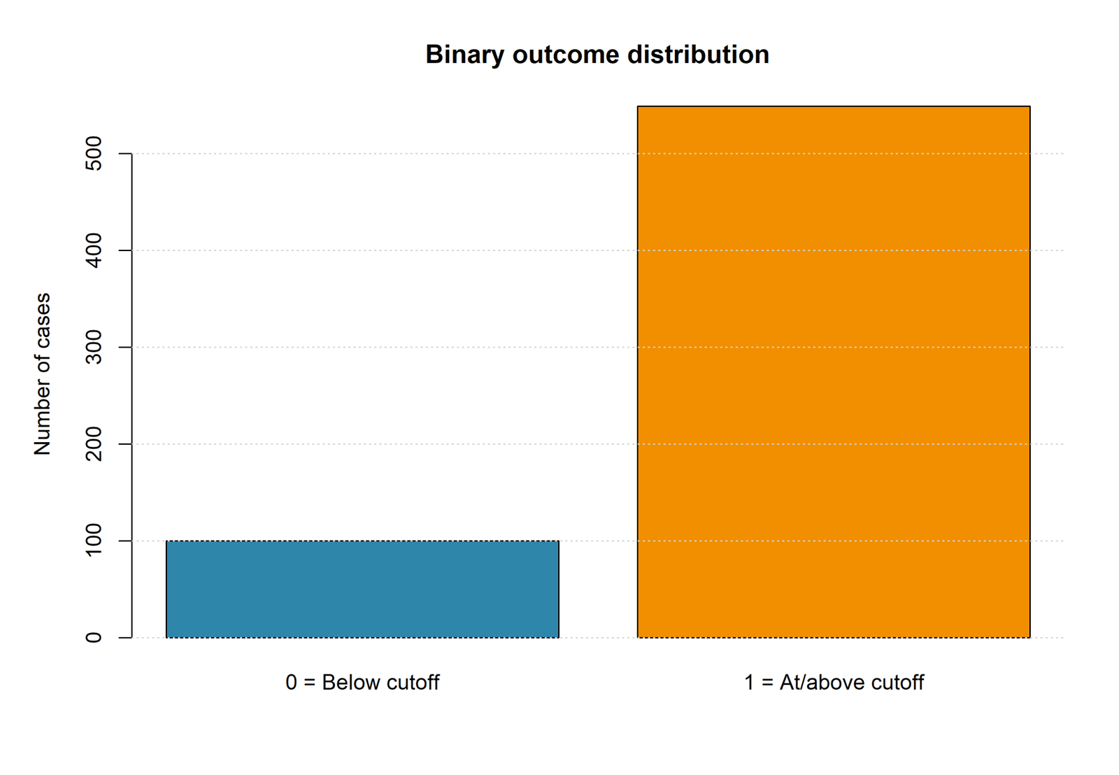
R Outcome Distribution
The response is imbalanced toward event status: 84.59% of observations have G3 ≥ 10. This makes sensitivity, specificity, and balanced accuracy necessary companions to overall accuracy.
R Probability Distribution
Most fitted probabilities lie near 1, while a smaller group lies close to 0. The mean probability of 0.84507 closely matches the observed event rate of 0.84592.
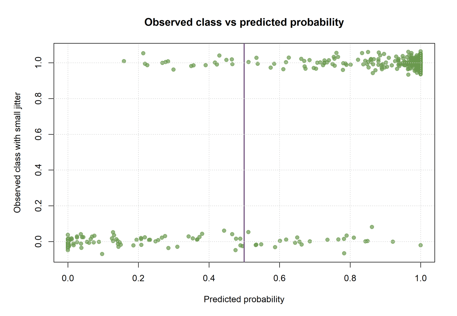
R Observed Class Versus Probability
Observed events are concentrated near high fitted probabilities, and many non-events receive low probabilities. The overlapping cases account for the 23 false positives and 17 false negatives.
R Probability Residuals
The two expected diagonal branches reflect Y − p̂ for binary outcomes. Most residuals are close to zero, while extreme values identify confident mistakes.
R Coefficient Plot
G2 and G1 have precise positive effects on the latent index, age is smaller but positive, and school MS is significantly negative. The remaining intervals include zero.
R Confusion Matrix
The model records 532 true positives, 77 true negatives, 23 false positives, and 17 false negatives. Sensitivity is 96.90%, while specificity is 77.00%.
R Probability by G1
Observed and fitted rates rise together from approximately one-quarter near G1 = 7 to almost certainty from G1 = 12 onward. The probability curve saturates at the upper end.
R Latent-Index Distribution
Most η values are positive and therefore correspond to probabilities above 0.50. The smaller negative tail contains observations classified as non-events.
Probit Regression Coefficient and Marginal-Effect Interpretation
Coefficient table
| Term | B | SE | z | p | 95% CI | Interpretation |
|---|---|---|---|---|---|---|
| Intercept | −12.814190 | 2.124178 | −6.0325 | <.001 | −16.977502 to −8.650878 | Latent score when numeric predictors equal zero and reference groups apply; not a realistic standalone probability scenario |
| school MS | −0.588822 | 0.237304 | −2.4813 | .01309 | −1.053930 to −0.123714 | MS has a lower latent pass score than GP, holding other variables fixed |
| sex M | −0.312284 | 0.226364 | −1.3796 | .16772 | −0.755950 to 0.131381 | Negative estimate relative to female, but interval includes zero |
| address U | −0.112358 | 0.225203 | −0.4989 | .61784 | −0.553748 to 0.329032 | Little adjusted evidence of an urban-rural difference |
| G1 | 0.331065 | 0.076525 | 4.3262 | <.001 | 0.181079 to 0.481052 | Higher G1 raises the latent score and event probability |
| G2 | 0.800302 | 0.113398 | 7.0575 | <.001 | 0.578046 to 1.022557 | Strongest positive latent-scale predictor |
| studytime | 0.089479 | 0.147093 | 0.6083 | .54298 | −0.198817 to 0.377775 | Small positive estimate with substantial uncertainty |
| failures | −0.185865 | 0.138095 | −1.3459 | .17833 | −0.456525 to 0.084796 | Negative estimate, but adjusted evidence is not conclusive |
| absences | −0.024443 | 0.023140 | −1.0563 | .29083 | −0.069797 to 0.020911 | Small negative estimate with interval crossing zero |
| age | 0.209143 | 0.094820 | 2.2057 | .02741 | 0.023299 to 0.394986 | Positive adjusted latent-scale association |
How to Interpret Sign and Significance
A positive coefficient means that increasing the predictor raises η and therefore raises p̂ for every fixed covariate pattern. A negative coefficient lowers both. Statistical significance indicates whether the coefficient is distinguishable from zero under the fitted model, not whether its probability effect is large in every part of the sample.
G2 has the strongest positive coefficient and the largest z statistic. Its 95% interval remains completely above zero. G1 is also positive and statistically precise. School MS is significantly negative relative to GP, and age is positive with a smaller z statistic. The remaining predictors have intervals that include zero.
Marginal Effects at the Probability Midpoint
| Predictor | φ(0) × B | Meaning at η = 0 |
|---|---|---|
| G2 | 0.3193 | Approximately 31.9 percentage points for a one-unit increase at the steepest point of the curve |
| G1 | 0.1321 | Approximately 13.2 percentage points per unit at η = 0 |
| age | 0.0834 | Approximately 8.3 percentage points per year at η = 0 |
| studytime | 0.0357 | Approximately 3.6 percentage points per category at η = 0 |
| failures | −0.0741 | Approximately −7.4 percentage points per failure at η = 0 |
| absences | −0.0098 | Approximately −1.0 percentage point per absence at η = 0 |
These values are marginal effects at η = 0, where the normal density is largest. They are not average marginal effects and should not be presented as constant effects. For categorical variables such as school, sex, and address, discrete probability changes are preferred.
Predictions, Classification, and Cutoff Choice
Worked calculator scenario
- G1 = 10
- G2 = 12
- studytime = 2
- failures = 0
- absences = 4
- age = 17
- school GP, male, urban
- η = 3.312053
- p̂ = 0.999537
- Predicted class = 1
Classification metrics at 0.50
- Accuracy = 93.84%
- Sensitivity = 96.90%
- Specificity = 77.00%
- Positive predictive value = 95.86%
- Negative predictive value = 81.91%
- Balanced accuracy = 86.95%
- F1 score = 96.38%
The workbook calculator first multiplies each input by its coefficient and adds the contributions to obtain η. Excel then applies NORM.S.DIST(η,TRUE). In the displayed scenario, the latent score of 3.3121 lies far into the positive tail, so the resulting probability is 0.9995.
A high probability is conditional on the fitted predictors and coding. It is not certainty, and it is not a causal statement. The result also reflects the strong contribution of G2 and G1. Changing a predictor when the starting probability is already near 1 produces only a small probability change because the probit curve is flat in the tail.
Choosing a Probability Cutoff
The 0.50 cutoff is convenient but not mandatory. If false negatives are especially costly, a lower cutoff can increase sensitivity. If false positives are especially costly, a higher cutoff can increase specificity. The cutoff should be selected using validation data, decision costs, and the intended application rather than chosen to maximize in-sample accuracy.
The outcome is imbalanced, so the threshold should not be judged only by accuracy. Balanced accuracy, class-specific recall, precision, and probability scoring rules provide a fuller evaluation. A confusion matrix should always state which outcome is the positive class.
Probit Regression Assumptions and Diagnostics
Main checks
- Correct event and reference coding
- Link and functional-form adequacy
- Separation and sparse cells
- Multicollinearity
- Residuals, leverage, and influence
- Calibration and discrimination
- Independence and clustering
- Out-of-sample validation
Current findings
- 549 events and 100 non-events
- Strong joint improvement over the null model
- Mean probability closely matches event rate
- High sensitivity and moderate specificity
- Several confident classification errors remain
- No evidence of failed coefficient estimation
Binary Outcome and Independent Observations
The dependent variable must contain two categories. Ordinary Probit Regression also assumes independent observations. Repeated measurements, students nested within classes, or observations clustered by site require a multilevel, random-effects, robust-clustered, or generalized-estimating approach.
Functional Form on the Probit Scale
Continuous predictors are assumed to contribute linearly to η unless transformations, splines, or interactions are included. A predictor can have a nonlinear probability relationship even with a linear latent coefficient, but the latent-index form itself still needs evaluation. Polynomial terms or a Generalized Additive Model may be appropriate if the probit-scale relationship is curved.
Multicollinearity
High predictor dependence inflates standard errors and destabilizes coefficient interpretation. Use Variance Inflation Factor, Tolerance Statistic, and a Correlation Matrix as supporting diagnostics. Grade predictors G1 and G2 are expected to be strongly related, so their coefficients describe adjusted rather than isolated associations.
Complete and Quasi-Complete Separation
Separation occurs when a predictor or combination of predictors perfectly identifies the outcome. Maximum-likelihood coefficients can then diverge or become unstable. Warning signs include enormous coefficients, enormous standard errors, failed convergence, or fitted probabilities of exactly 0 and 1 for complete groups. Penalized or Bayesian methods may be required.
Residuals and Influence
Raw residuals form two branches and have nonconstant variance by design. Pearson and deviance residuals are more appropriate for identifying unusual observations. Leverage and influence measures help determine whether a small number of cases controls the coefficient estimates. The extreme raw residuals in the chart should be traced to their covariate patterns.
Calibration
Calibration asks whether predicted probabilities agree with observed event frequencies. The overall mean prediction of 0.84507 is close to the observed rate of 0.84592, and the binned G1 chart shows close agreement. These are encouraging in-sample checks but do not replace validation calibration curves or calibration intercept and slope estimates.
Discrimination
Discrimination asks whether event cases tend to receive higher probabilities than non-event cases. The observed-versus-predicted chart and confusion matrix show strong separation, but a complete evaluation would also include an ROC curve and area under the curve. No AUC value should be invented when it is not part of the supplied output.
Model Comparison
AIC can compare Probit Regression with alternative probit specifications fitted to the same outcome and data. Comparisons with logistic regression should consider predictive validation, calibration, theoretical link choice, and interpretability rather than coefficient magnitude alone.
Sample Size
The analysis contains 100 non-events for nine slopes, which provides more information than a very sparse non-event sample. Nevertheless, effective sample size depends on predictor distributions, category frequencies, separation, and model complexity. Interaction terms or numerous indicators would require additional data.
Probit Regression in Python, R, SPSS and Excel
Python Probit Regression
Python can fit Probit Regression with statsmodels using either a discrete Probit class or a binomial generalized linear model with a probit link. The GLM route makes the link explicit and provides fitted probabilities, residuals, and likelihood-based output.
- Create the binary event from G3
- Declare categorical reference groups
- Fit the binomial-probit model
- Generate probabilities and classifications
- Calculate confusion-matrix metrics and log loss
Probit Regression in R
R uses glm(..., family = binomial(link = "probit")). Coefficients, confidence intervals, fitted probabilities, deviance residuals, and model-comparison measures can be produced with base R and supporting packages.
- Convert school, sex, and address to factors
- Set intended reference categories
- Fit with
glm() - Use
predict(type = "response") - Calculate marginal effects or probability scenarios
SPSS Probit Regression
SPSS can fit a binary probit link with GENLIN. The outcome category, reference categories, distribution, link, parameter estimates, goodness-of-fit measures, and saved predictions should be defined explicitly.
- Compute the 0/1 outcome
- Use binomial distribution and probit link
- Declare categorical factors
- Request parameter estimates and model fit
- Save predicted probabilities for diagnostics
Probit Regression in Excel
Excel is well suited to applying a fitted Probit Regression equation. It can calculate η with SUMPRODUCT, transform η with NORM.S.DIST, and assign a class from a chosen cutoff. Estimating coefficients from scratch requires numerical optimization and is less convenient than dedicated statistical software.
- Store coefficients in fixed cells
- Code categorical indicators as 0 or 1
- Calculate the latent score
- Apply the standard normal CDF
- Compare probability with the cutoff
Code: Expand Only the Software You Need
Python Probit Regression with statsmodels GLM
from pathlib import Path
import numpy as np
import pandas as pd
import statsmodels.api as sm
import statsmodels.formula.api as smf
from sklearn.metrics import confusion_matrix, log_loss

folder = Path(__file__).resolve().parent if "__file__" in globals() else Path.cwd()
data_path = folder / "dataset.csv"
df = pd.read_csv(data_path)

df["probit_pass"] = (df["G3"] >= 10).astype(int)
df["school"] = pd.Categorical(df["school"], categories=["GP", "MS"])
df["sex"] = pd.Categorical(df["sex"], categories=["F", "M"])
df["address"] = pd.Categorical(df["address"], categories=["R", "U"])

formula = (
    "probit_pass ~ C(school) + C(sex) + C(address) + "
    "G1 + G2 + studytime + failures + absences + age"
)

model = smf.glm(
    formula=formula,
    data=df,
    family=sm.families.Binomial(link=sm.families.links.Probit())
).fit()

probability = model.predict(df)
predicted_class = (probability >= 0.50).astype(int)
tn, fp, fn, tp = confusion_matrix(df["probit_pass"], predicted_class).ravel()

print(model.summary())
print({"TN": tn, "FP": fp, "FN": fn, "TP": tp})
print("Accuracy:", (tn + tp) / len(df))
print("Log loss:", log_loss(df["probit_pass"], probability))
R Probit Regression with glm()
data <- read.csv("dataset.csv", stringsAsFactors = FALSE)

data$probit_pass <- ifelse(data$G3 >= 10, 1, 0)
data$school <- relevel(factor(data$school), ref = "GP")
data$sex <- relevel(factor(data$sex), ref = "F")
data$address <- relevel(factor(data$address), ref = "R")

model <- glm(
  probit_pass ~ school + sex + address + G1 + G2 +
    studytime + failures + absences + age,
  data = data,
  family = binomial(link = "probit")
)

summary(model)
confint.default(model)

p_hat <- predict(model, type = "response")
class_hat <- ifelse(p_hat >= 0.50, 1, 0)
table(Actual = data$probit_pass, Predicted = class_hat)

log_loss <- -mean(
  data$probit_pass * log(p_hat) +
  (1 - data$probit_pass) * log(1 - p_hat)
)
print(log_loss)
SPSS GENLIN syntax with a Probit link
COMPUTE probit_pass = (G3 >= 10).
VARIABLE LEVEL probit_pass (NOMINAL).
EXECUTE.

GENLIN probit_pass (REFERENCE=FIRST) BY school sex address
  WITH G1 G2 studytime failures absences age
  /MODEL school sex address G1 G2 studytime failures absences age
    DISTRIBUTION=BINOMIAL LINK=PROBIT
  /CRITERIA METHOD=FISHER(1) SCALE=1 COVB=MODEL
    MAXITERATIONS=100 MAXSTEPHALVING=5
  /PRINT CPS DESCRIPTIVES MODELINFO FIT SUMMARY SOLUTION
  /SAVE PREDVAL(predicted_probability).

COMPUTE predicted_class = (predicted_probability >= .50).
CROSSTABS
  /TABLES=probit_pass BY predicted_class
  /CELLS=COUNT ROW COLUMN.
Excel probability and classification formulas
Linear predictor:
=Intercept + SUMPRODUCT(Input_Range, Coefficient_Range)

Predicted probability:
=NORM.S.DIST(Linear_Predictor_Cell,TRUE)

Predicted class at a 0.50 cutoff:
=IF(Predicted_Probability_Cell>=Cutoff_Cell,1,0)

Raw probability residual:
=Observed_Class_Cell-Predicted_Probability_Cell

Correct classification indicator:
=--(Observed_Class_Cell=Predicted_Class_Cell)
Advanced Probit Regression Topics
Probit Regression Explained for Beginners
Probit Regression predicts the probability of a yes/no outcome. It first creates a weighted score from the predictors, then converts that score to probability with the standard normal cumulative distribution.
What Is a Probit Regression Model?
It is a binomial generalized linear model with a probit link. The inverse normal CDF of the event probability is modeled as a linear function of predictors.
Probit Regression Equation
The probability equation is p = Φ(Xβ). The linked equation is Φ⁻¹(p) = Xβ. Categorical variables enter through indicator contrasts.
Latent Variable in Probit Regression
The binary outcome can be viewed as a thresholded latent variable Y* = Xβ + ε, with ε following a standard normal distribution. The event occurs when Y* crosses zero.
When to Use Probit Regression
Use it for a binary outcome when a latent normally distributed threshold process is plausible, when the probit link is standard in the field, or when it offers useful comparison with logistic regression.
Probit Regression Versus Logistic Regression
Both models estimate binary probabilities. Probit uses a normal CDF; logistic uses a logistic CDF and supports direct odds-ratio interpretation. Predicted probabilities are often similar in ordinary data ranges.
How to Interpret Probit Regression Coefficients
The coefficient is a change in the latent z-score, not a constant probability effect. Its sign gives the probability direction; practical magnitude comes from marginal effects or predicted scenarios.
Marginal Effects in Probit Regression
For a continuous variable, the marginal effect is φ(Xβ)β. It varies by observation. Analysts may report effects at representative values or average marginal effects across the sample.
Discrete Changes for Binary Predictors
For an indicator, compute the fitted probability with the indicator at 0 and at 1 while holding other values fixed. The difference is easier to interpret than the latent coefficient.
Probit Regression Assumptions
Assumptions include a binary outcome, independent observations, a correct latent-index form, no perfect multicollinearity, no destructive separation, and sufficient information in both outcome groups.
McFadden Pseudo-R-Squared
McFadden pseudo-R² compares the fitted and null log likelihoods. It is not the percentage of outcome variance explained and should not be interpreted like ordinary R².
Likelihood-Ratio Test
The likelihood-ratio test compares nested models through twice the difference in log likelihood. Here χ²(9) = 379.308, p < .001, showing strong joint improvement over the intercept-only model.
Probit Regression Classification
Classification converts probabilities to classes with a threshold. Because threshold choice is external to estimation, report the cutoff and class-specific error measures.
Calibration of Probit Probabilities
Calibration measures agreement between predicted probabilities and observed frequencies. Evaluate it with calibration plots, grouped rates, and validation calibration slope and intercept.
ROC Curve and AUC
ROC analysis evaluates discrimination over all cutoffs. AUC should be computed from the fitted probabilities and reported only when it has actually been calculated.
Residuals in Probit Regression
Raw residuals are intuitive but have a two-branch pattern. Pearson and deviance residuals are more suitable for identifying poorly fitted cases in a binary model.
Separation in Probit Regression
Complete separation can cause coefficients to diverge and standard errors to become unstable. Penalized likelihood, Bayesian priors, simpler models, or additional data may be needed.
Interaction Effects
An interaction coefficient changes the latent index, but its probability-scale effect varies with all predictors. Plot predicted probabilities or marginal effects across meaningful values.
Nonlinear Predictors
Squared terms, splines, or other transformations can be added to the latent predictor. Keep hierarchical lower-order terms and validate the added flexibility.
Ordered Probit Regression
Ordered outcome methods extend the threshold idea to more than two ordered categories. Multiple cut points map one latent variable to the observed ordered response.
Multinomial Probit Regression
Multinomial probit handles more than two unordered choices and can model correlated latent utilities. It is more computationally demanding than binary Probit Regression.
Bivariate Probit Regression
Bivariate probit jointly models two binary outcomes with correlated latent errors. It is appropriate when the two decisions are related beyond observed predictors.
Panel Probit Regression
Panel probit methods account for repeated binary outcomes over units and time. Random-effects and correlated-random-effects assumptions require careful evaluation.
Bayesian Probit Regression
Bayesian Regression places priors on coefficients and produces posterior probability summaries. Data augmentation makes the latent-normal representation computationally convenient.
Endogenous Probit Models
When a predictor is endogenous, ordinary Probit Regression can be biased. Instrumental-variable or control-function approaches require strong identification assumptions and specialized software.
Probit Regression in Python
Statsmodels supports both discrete Probit and binomial GLM with a probit link. Use a reproducible preprocessing pipeline and validate probability performance.
Probit Regression in R
Use glm(..., family=binomial(link="probit")), then obtain fitted probabilities, confidence intervals, marginal effects, residuals, and validation metrics.
Probit Regression in SPSS
Use GENLIN with a binomial distribution and probit link. Explicitly set outcome and reference coding and save fitted probabilities for diagnostics.
Probit Regression in Excel
Excel can apply a fitted equation with NORM.S.DIST. Dedicated statistical software is preferable for maximum-likelihood estimation and inferential diagnostics.
How to Report Probit Regression
Report the event definition, reference categories, sample size, coefficients and confidence intervals, likelihood-based fit, pseudo-R², probability interpretation, cutoff, classification metrics, and validation approach.
APA-Style Reporting
The fitted model improved significantly over the intercept-only model, likelihood-ratio χ²(9) = 379.31, p < .001. The model had log likelihood = −89.24, AIC = 198.48, McFadden pseudo-R² = .680, and log loss = .138.
G2 was positively associated with the latent pass propensity, B = 0.800, SE = 0.113, z = 7.057, p < .001, 95% CI [0.578, 1.023]. G1 was also positive, B = 0.331, SE = 0.077, z = 4.326, p < .001, 95% CI [0.181, 0.481]. School MS was negative relative to school GP, B = −0.589, SE = 0.237, z = −2.481, p = .013, 95% CI [−1.054, −0.124], and age was positive, B = 0.209, SE = 0.095, z = 2.206, p = .027, 95% CI [0.023, 0.395].
At a probability cutoff of .50, the model classified 93.84% of observations correctly, with sensitivity of 96.90% and specificity of 77.00%. Predicted probabilities should be emphasized because latent-scale coefficients do not represent constant probability changes.
Publication Checklist
Include
- Binary outcome definition and event category
- Reference groups for categorical predictors
- Sample size, event count, and non-event count
- Probit link and estimation method
- Coefficient, SE, z, p, and confidence interval
- Likelihood-ratio test, log likelihood, and AIC
- Clear pseudo-R² terminology
- Predicted probabilities or marginal effects
- Declared classification cutoff
- Confusion matrix and class-specific metrics
- Calibration, influence, and validation checks
- Software and reproducible code
Avoid
- Calling probit coefficients odds ratios
- Interpreting coefficients as fixed percentage changes
- Calling pseudo-R² variance explained
- Reporting accuracy without the class distribution
- Hiding the event and reference categories
- Choosing 0.50 without considering error costs
- Ignoring separation or sparse categories
- Using in-sample accuracy as future performance
- Claiming causation from observational associations
- Inventing ROC AUC or marginal effects not calculated
Use Confidence Interval, P-Value, Statistical Power, and Type I and Type II Error terminology only where it matches the analysis and decision context.
Downloads and Chart Resources
Probit Regression R ReportComplete R report with model tables and chart sequence
Binary Outcome DistributionPass and non-pass counts used by the model
Predicted Probability DistributionFitted probabilities and the 0.50 cutoff
Observed Versus Predicted ProbabilityObserved class compared with fitted event probability
Probability Residual PlotObserved class minus fitted probability
Probit Coefficient PlotLatent-scale estimates and 95% confidence intervals
Confusion MatrixTN, FP, FN, and TP at the 0.50 cutoff
Probability by G1Binned fitted probabilities and observed event rates
Linear Predictor DistributionLatent probit z-scores and the η = 0 boundary
Frequently Asked Questions
What is Probit Regression?
Probit Regression is a binary-response model that converts a linear predictor into an event probability with the standard normal cumulative distribution function.
When should Probit Regression be used?
Use it for a binary outcome when a latent normal threshold interpretation is plausible or when the probit link is preferred by theory, convention, or comparative modeling.
What is the Probit Regression formula?
The probability formula is P(Y=1|X) = Φ(Xβ), and the linked form is Φ⁻¹[P(Y=1|X)] = Xβ.
How is Probit Regression different from logistic regression?
Probit uses the standard normal CDF, while logistic regression uses the logistic CDF. Logistic coefficients support odds ratios; probit coefficients are interpreted through latent z-scores and marginal probabilities.
How do I interpret a positive probit coefficient?
A positive coefficient raises the latent index and therefore increases the event probability, holding other predictors constant. The probability increase varies across cases.
Can probit coefficients be converted to odds ratios?
No. Exponentiated probit coefficients are not odds ratios. Use predicted probabilities, marginal effects, or discrete changes.
What does McFadden pseudo-R-squared mean?
It measures improvement in log likelihood relative to an intercept-only model. It is not the percentage of variance explained.
What is the event in this example?
The event equals 1 when final grade G3 is at least 10. There are 549 events and 100 non-events.
Which predictors are statistically significant?
G1, G2, age, and school MS are statistically significant at the .05 level. G1, G2, and age are positive; school MS is negative relative to GP.
What is the strongest predictor?
G2 has the largest positive latent-scale coefficient and z statistic, B = 0.8003, z = 7.057, p < .001.
How accurate is the fitted model?
At a 0.50 cutoff, in-sample accuracy is 93.84%, sensitivity is 96.90%, and specificity is 77.00%.
Why is specificity lower than sensitivity?
Pass outcomes dominate the sample and are strongly predicted by earlier grades. Non-pass cases include more overlap with the pass covariate profile, producing 23 false positives.
Is a 0.50 cutoff required?
No. Select a cutoff from validation data and the relative costs of false positives and false negatives.
How do I calculate a probit probability in Excel?
Calculate η from the coefficient-weighted inputs, then use NORM.S.DIST(η,TRUE).
How is Probit Regression fitted in Python?
Use statsmodels Probit or a binomial GLM with a probit link, then obtain fitted probabilities and evaluate them with appropriate metrics.
How is Probit Regression fitted in R?
Use glm(..., family = binomial(link = "probit")), then calculate predictions, confidence intervals, residuals, and marginal effects.
How is Probit Regression performed in SPSS?
Use GENLIN with a binomial distribution and probit link, declare categorical factors and reference groups, and save predicted probabilities.
What are the main Probit Regression assumptions?
The outcome must be binary, observations should be appropriately independent, the latent-index form should be suitable, predictors should not be perfectly collinear, and separation should not destabilize estimation.
Can Probit Regression include interactions and nonlinear terms?
Yes. Interactions, polynomial terms, and splines can enter the latent predictor, but their probability effects should be graphed or summarized with marginal effects.
Does high in-sample accuracy guarantee future performance?
No. Use cross-validation or a separate test sample to estimate future calibration, discrimination, and classification accuracy.
Probit Regression Conclusion
Probit Regression is a probability model for binary outcomes that maps a linear predictor through the standard normal cumulative distribution. It is particularly useful when the observed yes/no outcome can be interpreted as a latent continuous propensity crossing a threshold.
In this 649-observation analysis, 549 cases meet the G3 pass criterion and 100 do not. The fitted model improves strongly over the intercept-only model, with likelihood-ratio χ²(9) = 379.31, p < .001, AIC = 198.48, and McFadden pseudo-R² = .680.
G2 and G1 are the principal positive predictors, age has a smaller positive coefficient, and school MS has a negative adjusted coefficient relative to GP. At the 0.50 cutoff, accuracy is 93.84%, sensitivity is 96.90%, and specificity is 77.00%.
The most defensible interpretation is probability based. Coefficients indicate movement on a latent z scale, while the real-world effect depends on the observation’s starting position on the probit curve. Predicted probabilities, marginal effects, class-specific metrics, and validation should therefore accompany the coefficient table.

