
Mediated Regression: Formula, Interpretation, SPSS, Python, R and Excel Guide
Mediated Regression tests whether the association between an independent variable and an outcome operates partly through an intervening variable. This worked analysis uses G1 as X, G2 as the mediator and G3 as Y, controls student background variables, estimates every path, and evaluates the indirect effect with 1,000 bootstrap samples.
G1 → G2 → G3
Indirect effect 0.7748
SPSS · Python · R · Excel
Mediated Regression Model Overview
Beginner explanation: Mediated Regression is used when you believe one variable affects another variable partly through a middle step. In this example, G1 is the earlier grade, G2 is the middle grade, and G3 is the final grade. The main question is: Does G1 help predict G3 partly because students with higher G1 scores also tend to have higher G2 scores?
The method separates the relationship into three simple pieces. First, it checks whether G1 predicts G2. Second, it checks whether G2 predicts G3 after G1 is already included. Third, it checks whether G1 still has a direct relationship with G3 after G2 is included. This is why Mediated Regression is easier to understand when you think of it as a chain: G1 → G2 → G3.
If you are new to regression, read Correlation vs Regression first. Correlation tells you whether two variables move together, while regression estimates how much the outcome changes when a predictor changes and other variables are controlled. You may also find Pearson Correlation useful for understanding the simple pairwise relationships before the regression equations are fitted.
The dependent variable in the final equation is G3. G1 is the independent variable, G2 is the mediator, and the remaining variables are controls. These controls help compare students who are similar in studytime, failures, absences, age, maternal education, school, sex and address.
Quick Answer: Mediated Regression Result
Effect decomposition
- Total effect c = 0.908578
- Direct effect c′ = 0.133732
- Indirect effect a×b = 0.774846
- c ≈ c′ + a×b
Bootstrap decision
- Python CI [0.679190, 0.871526]
- R CI [0.676560, 0.864288]
- Both intervals exclude zero
- Mediated Regression is supported
What these numbers mean in plain language: students with higher G1 scores usually have higher G2 scores, and students with higher G2 scores usually have higher G3 scores. Most of the statistical relationship between G1 and G3 is therefore carried through G2. The remaining direct effect of G1 is much smaller.
The confidence interval is the most important decision tool. A confidence interval gives a range of plausible values for the indirect effect. Because both the Python and R intervals stay above zero, the indirect effect is supported. A p-value can be useful, but the interval also shows the size and direction of the effect.
Table of Contents
- What Mediated Regression is
- Beginner terminology
- How the paths work
- Variables and coding
- Direct, indirect and total effects
- Results at a glance
- R chart stories explained first
- Python charts in paired validation layout
- SPSS cross-software results
- Diagnostics and assumptions
- SPSS, Python, R and Excel
- Excel formulas and workbook
- Code
- Beginner study guide
- Advanced interpretation
- APA-style reporting
- Publication checklist
- Downloads
- Related guides
- FAQs
What Is Mediated Regression?
Mediated Regression is a regression-based approach to a single-mediator model. The first equation predicts the mediator from X and covariates. The second predicts Y from X, the mediator and covariates. A separate total-effect equation predicts Y from X and covariates without the mediator.
The coefficient of X in the mediator equation is path a. The coefficient of M in the outcome equation is path b. The coefficient of X in the total-effect equation is c, and the coefficient of X after M is included is c′. The indirect effect is the product a×b and is also approximately equal to c−c′ when the same linear specification and sample are used.
Mediated Regression is sometimes described as mediation analysis using regression. The method is not simply a comparison of whether c is significant before M enters and non-significant afterward. Contemporary interpretation focuses on the indirect effect and its bootstrap confidence interval.
Mediated Regression Terms Explained for Beginners
The three main variables
- X or predictor: the starting variable. Here it is G1.
- M or mediator: the middle variable that may carry part of the relationship. Here it is G2.
- Y or outcome: the final variable being explained. Here it is G3.
The four path labels
- Path a: how much G2 changes when G1 increases.
- Path b: how much G3 changes when G2 increases, after controlling G1.
- Total effect c: the G1–G3 relationship before G2 is added.
- Direct effect c′: the G1–G3 relationship after G2 is added.
The indirect effect is calculated as path a multiplied by path b. It represents the part of the G1–G3 relationship that passes through G2. The direct effect represents the part that remains after G2 is included.
If you want to understand what “controlling for other variables” means, read Partial Correlation and Semi-Partial Correlation. These guides explain how a relationship changes after the influence of other variables is removed.
How Mediated Regression Works
Predict G2 from G1 and the covariates.
Predict G3 from G1, G2 and the covariates.
Resample rows and estimate the distribution of a×b.
Step 1: Predict G2 from G1
The first equation asks whether G1 predicts the mediator G2. The estimated slope is path a. Here, path a = 0.879067. This means that after the control variables are held constant, one additional G1 point is associated with about 0.879 additional G2 points.
Step 2: Predict G3 from G1 and G2
The second equation includes both G1 and G2. The coefficient for G2 is path b, and the coefficient for G1 is the direct effect c′. Path b = 0.881441, so one additional G2 point is associated with about 0.881 additional G3 points when G1 and the control variables are held constant.
Step 3: Calculate the indirect effect
Multiply path a by path b: 0.879067 × 0.881441 = 0.774846. This is the estimated indirect effect. In practical terms, about 0.775 G3 points of the G1–G3 association are represented by the pathway through G2.
Step 4: Compare the indirect and direct effects
The direct effect c′ is 0.133732. The indirect effect is much larger than the direct effect. This is why the article concludes that G2 carries most of the adjusted relationship between G1 and G3.
To understand why adjusted and unadjusted model fit can differ, see Adjusted R-Squared. It explains how model fit is evaluated after accounting for the number of predictors.
Mediated Regression Variables Used and Coding
| Variable | Role | Definition | Type |
|---|---|---|---|
| G1 | Independent variable X | First-period grade; mean 11.399, SD 2.745, range 0–19. | Continuous |
| G2 | Mediator M | Second-period grade; mean 11.570, SD 2.914, range 0–19. | Continuous |
| G3 | Outcome Y | Final grade; mean 11.906, SD 3.231, range 0–19. | Continuous |
| studytime | Covariate | Weekly study-time category. | Ordinal |
| failures | Covariate | Number of past class failures. | Count/ordinal |
| absences | Covariate | School absence count. | Count |
| age | Covariate | Student age in years. | Continuous |
| Medu | Python/R covariate | Mother’s education level. | Ordinal |
| school | Categorical covariate | MS compared with GP. | Binary contrast |
| sex | Categorical covariate | Male compared with female. | Binary contrast |
| address | Categorical covariate | Urban compared with rural. | Binary contrast |
| higher, internet | SPSS-only additional covariates | Higher-education intention and internet-access indicators. | Binary contrasts |
Mediated Regression Direct, Indirect and Total Effects
| Effect | Estimate | Uncertainty | Confidence interval / evidence | Decision | Interpretation |
|---|---|---|---|---|---|
| Path a: G1 → G2 | 0.879067 | SE 0.024436 | 95% CI [0.831082, 0.927052] | p < .001 | Higher G1 predicts higher G2. |
| Path b: G2 → G3 | G1 | 0.881441 | Reported in outcome model | Positive and highly significant | p < .001 | G2 predicts G3 after G1 and covariates. |
| Total effect c: G1 → G3 | 0.908578 | SE 0.030179 | 95% CI [0.849315, 0.967841] | p < .001 | G1 predicts G3 before G2 enters. |
| Direct effect c′: G1 → G3 | G2 | 0.133732 | Reported in outcome model | Positive and significant | p < .001 | A smaller G1 effect remains after G2 enters. |
| Indirect effect a×b | 0.774846 | Bootstrap mean 0.7752 Python; 0.7727 R | Python CI [0.679190, 0.871526]; R CI [0.676560, 0.864288] | CI excludes zero | Mediated Regression is supported. |
| Proportion mediated | 0.852811 | Indirect / total | About 85.28% | Descriptive ratio | Most of the G1–G3 association operates through G2. |
The total effect of 0.908578 means that, before G2 enters, one additional G1 point is associated with approximately 0.909 additional G3 points after the covariates are controlled. When G2 enters, the G1 coefficient falls to 0.133732.
The indirect effect of 0.774846 is the estimated portion carried through G2. Dividing the indirect effect by the total effect gives 0.852811, or approximately 85.28%. Because c′ remains positive and statistically different from zero, the model contains both an indirect pathway and a smaller direct pathway.
How to read this table as a beginner
Start with the indirect effect row. It is the main result of the mediation analysis. Then look at the confidence interval. If the interval includes zero, the indirect effect is not clearly supported. Here, both software intervals are fully positive.
Next, compare the indirect effect with the direct effect. The indirect effect is 0.774846, while the direct effect is 0.133732. This shows that the pathway through G2 is much larger than the remaining G1–G3 relationship.
The size of an effect and its statistical evidence are different ideas. Use the Effect Size guide to understand magnitude, and the Confidence Interval guide to understand precision.
Mediated Regression Results at a Glance
G2 predicted from G1 and covariates
G3 predicted without G2
G3 predicted with G2
SD = 0.0512
SD = 0.0480
Successful in both workflows
| Model | Dependent variable | Predictors excluding intercept | R² | Adjusted R² | F | p | Additional fit information |
|---|---|---|---|---|---|---|---|
| Path a mediator model | G2 | 9 | 0.7575 | 0.7541 | 221.7512 | < .001 | Python AIC 2329.4646; R AIC 2331.465 |
| Total-effect model | G3 | 9 | 0.6991 | 0.6949 | 164.9682 | < .001 | Python AIC 2603.4667; R AIC 2605.467 |
| Direct + mediator model | G3 | 10 | 0.8524 | 0.8501 | 368.3748 | < .001 | Python AIC 2143.3400; R AIC 2145.340 |
| SPSS path a model | G2 | 10 | 0.757 | 0.754 | 199.203 | < .001 | Includes higher and internet; SEE 1.446249 |
| SPSS total model | G3 | 10 | 0.701 | 0.696 | 149.337 | < .001 | Includes higher and internet; SEE 1.781348 |
| SPSS direct + mediator model | G3 | 11 | 0.852 | 0.850 | 334.569 | < .001 | Includes higher and internet; SEE 1.251626 |
Download the Mediated Regression Outputs
The same resources appear again in the complete Downloads section.
R Mediated Regression Chart Stories Explained First
How to use this section: do not try to memorize every number. For each chart, first identify the variables, then read the exact values, then read the statistical meaning. The final box tells you which assumption or diagnostic should be checked next.
The R charts are presented first because their exported design is clearer. Each R figure receives the full four-box explanation before the corresponding Python validation charts appear.
Mediated Regression readers should use these R figures as the primary visual narrative and the later Python pairs as cross-software confirmation.
R Chart 1: Mediated Regression Path Diagram
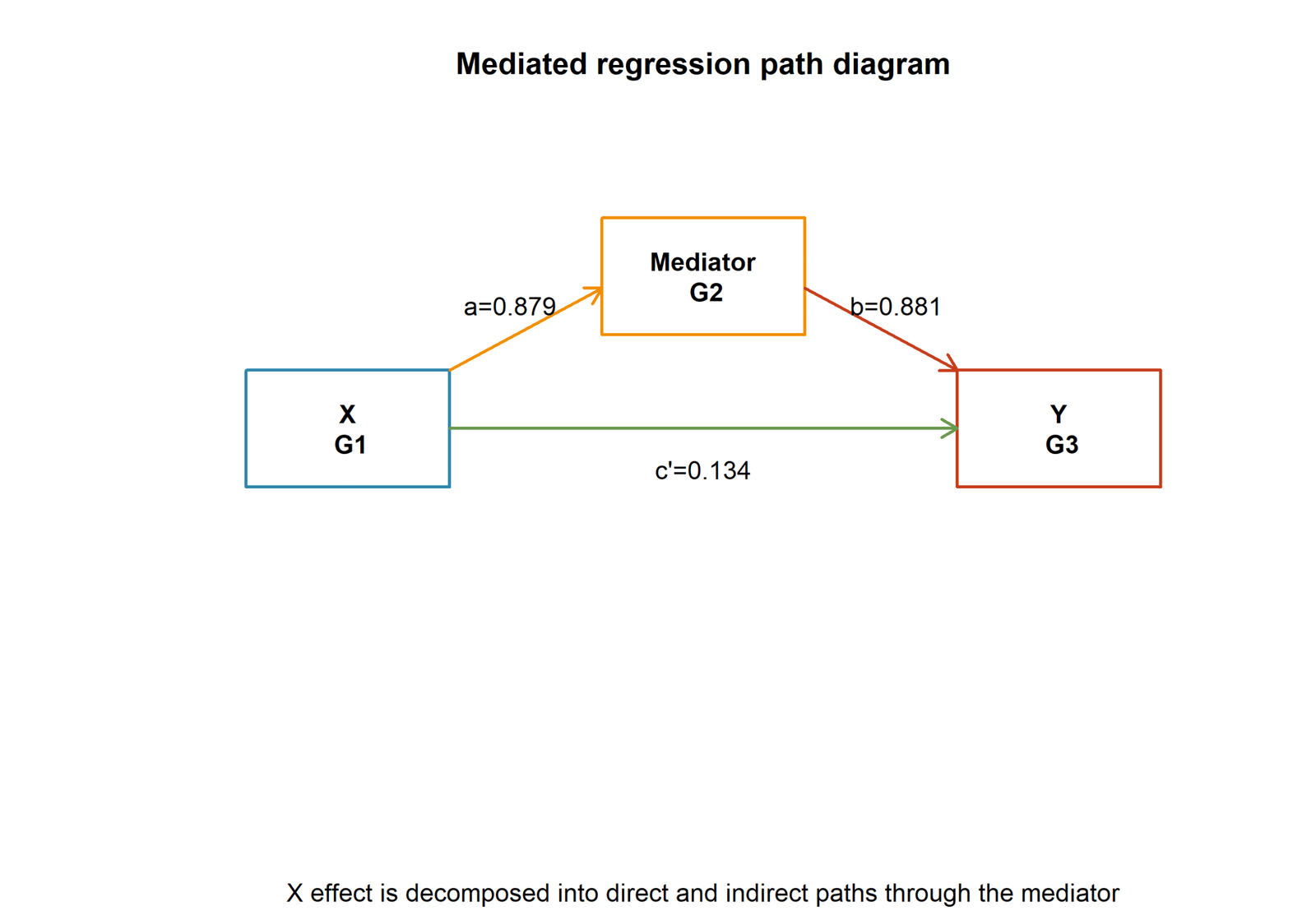
The diagram summarizes the complete single-mediator structure. G1 is the independent variable, G2 is the mediator and G3 is the outcome. Covariates are included in each regression equation but are omitted from the visual to preserve readability.
Path a is 0.879067, path b is 0.881441, total effect c is 0.908578, direct effect c′ is 0.133732, and a×b is 0.774846.
The total G1 effect is divided into a large indirect component through G2 and a smaller remaining direct component. The direct coefficient remains positive, so the pattern is partial rather than zero-direct-effect mediation.
Use the bootstrap interval as the primary indirect-effect decision. Do not conclude mediation only because paths a and b are individually significant.
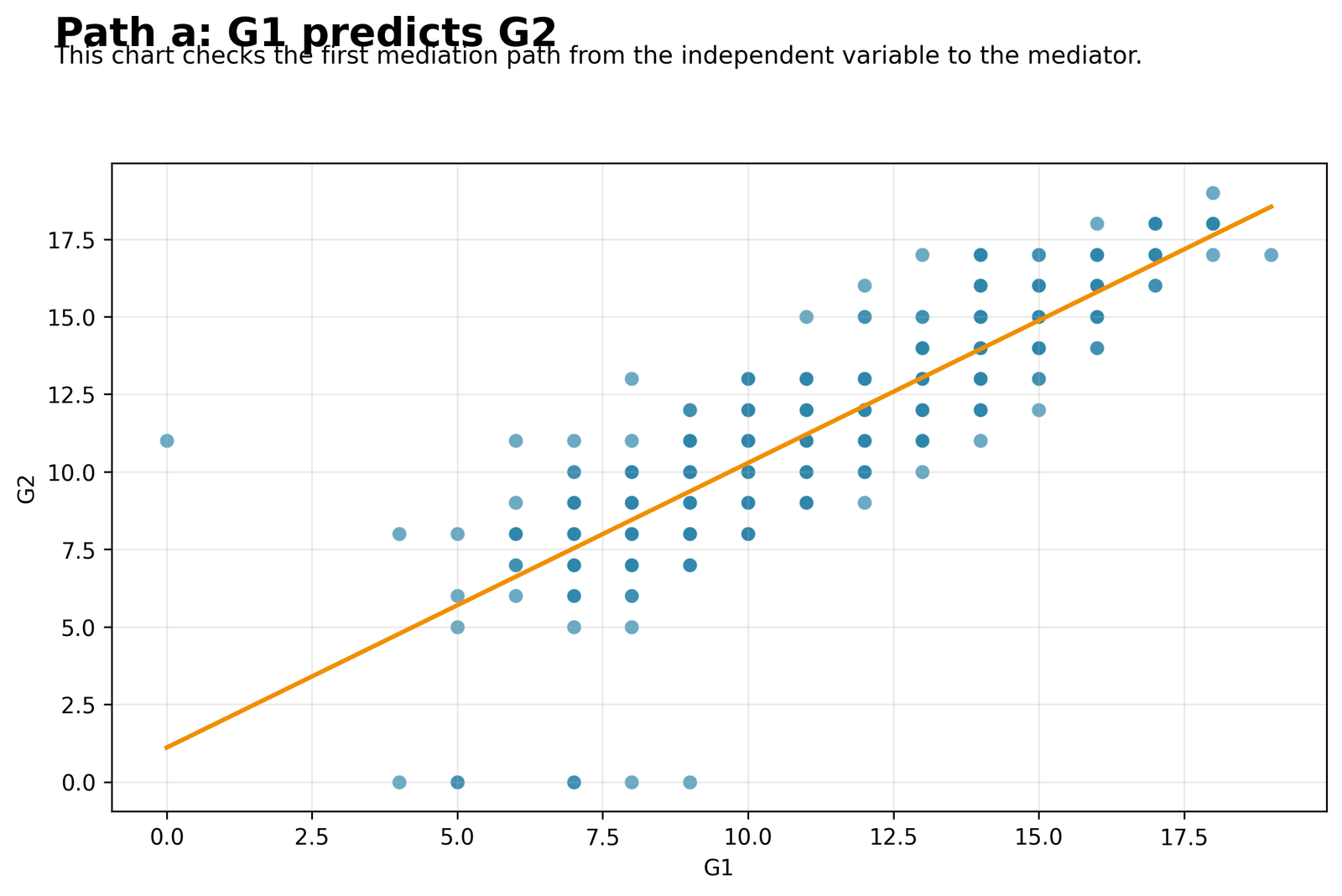
R Chart 2: Path a from G1 to G2
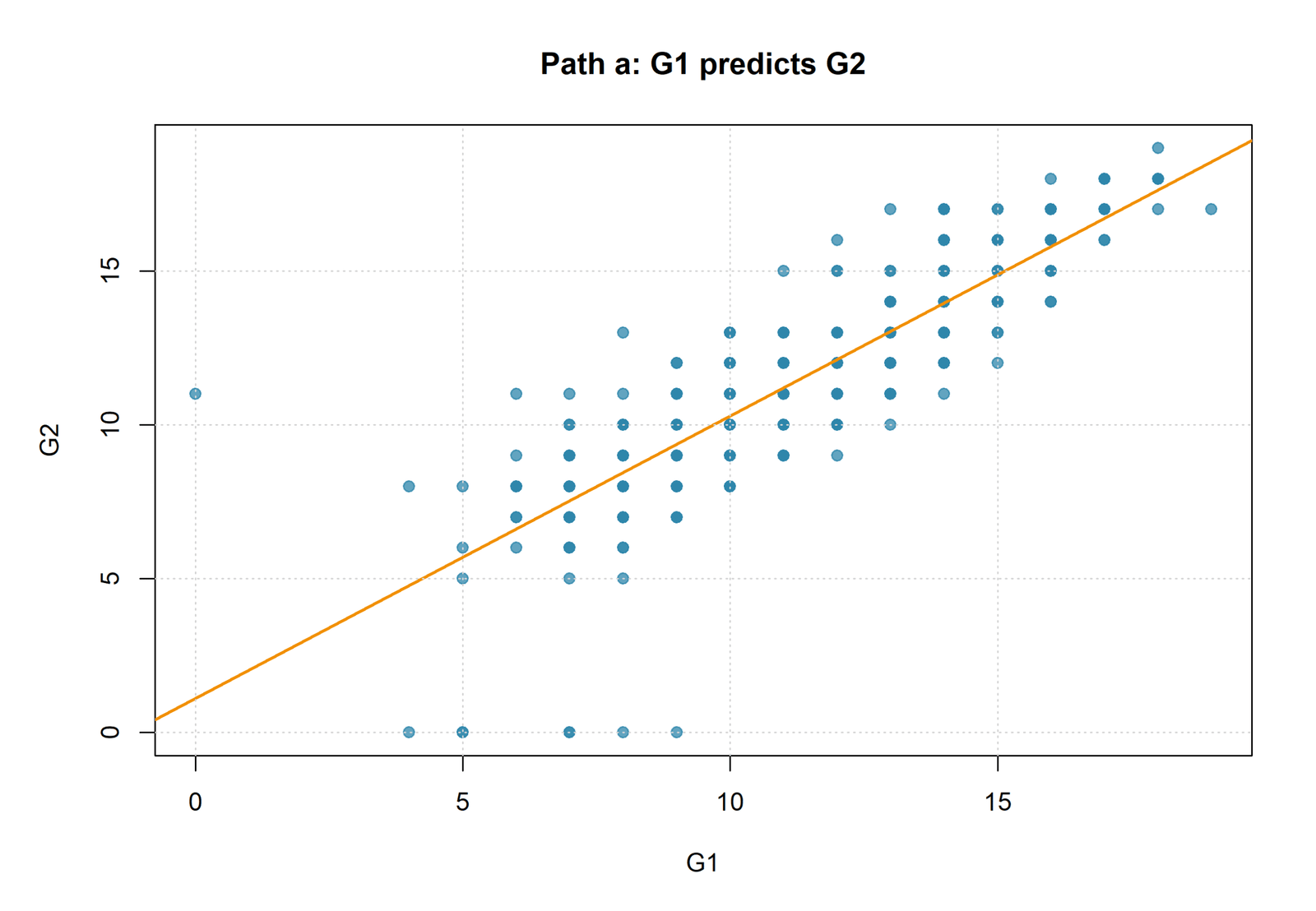
The figure displays the first regression equation in the mediated pathway. It asks whether variation in the independent variable is associated with variation in the proposed mediator.
a = 0.879067, SE = 0.024436, t = 35.9740, p < .001, 95% CI [0.831082, 0.927052]. The mediator model has R² = 0.7575.
Holding studytime, failures, absences, age, Medu, school, sex and address constant, each additional G1 point is associated with about 0.879 additional G2 points.
Inspect linearity, residual spread and influential observations. A strong path a is compatible with mediation but is not sufficient evidence by itself.
R Chart 3: Path b from G2 to G3
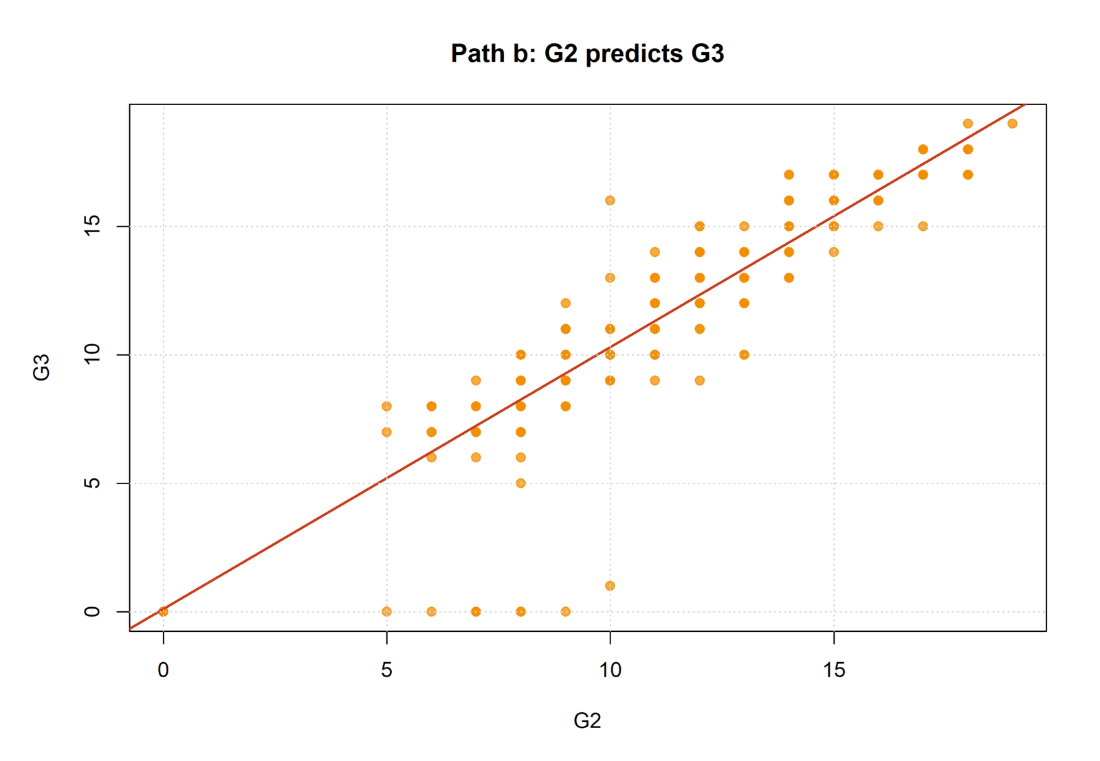
This plot represents the mediator-to-outcome component. The coefficient is conditional on G1, which distinguishes path b from the simple G2–G3 correlation.
Path b is 0.881441. The complete outcome model has R² = 0.8524, adjusted R² = 0.8501, and F = 368.3748, p < .001.
Students with the same G1 and covariate profile are expected to differ by about 0.881 G3 points for each one-point difference in G2. G2 carries substantial information from earlier performance to the final grade.
Interpret the coefficient conditionally and examine multicollinearity between G1 and G2. A strong b path can remain estimable even when the two grades are highly correlated.
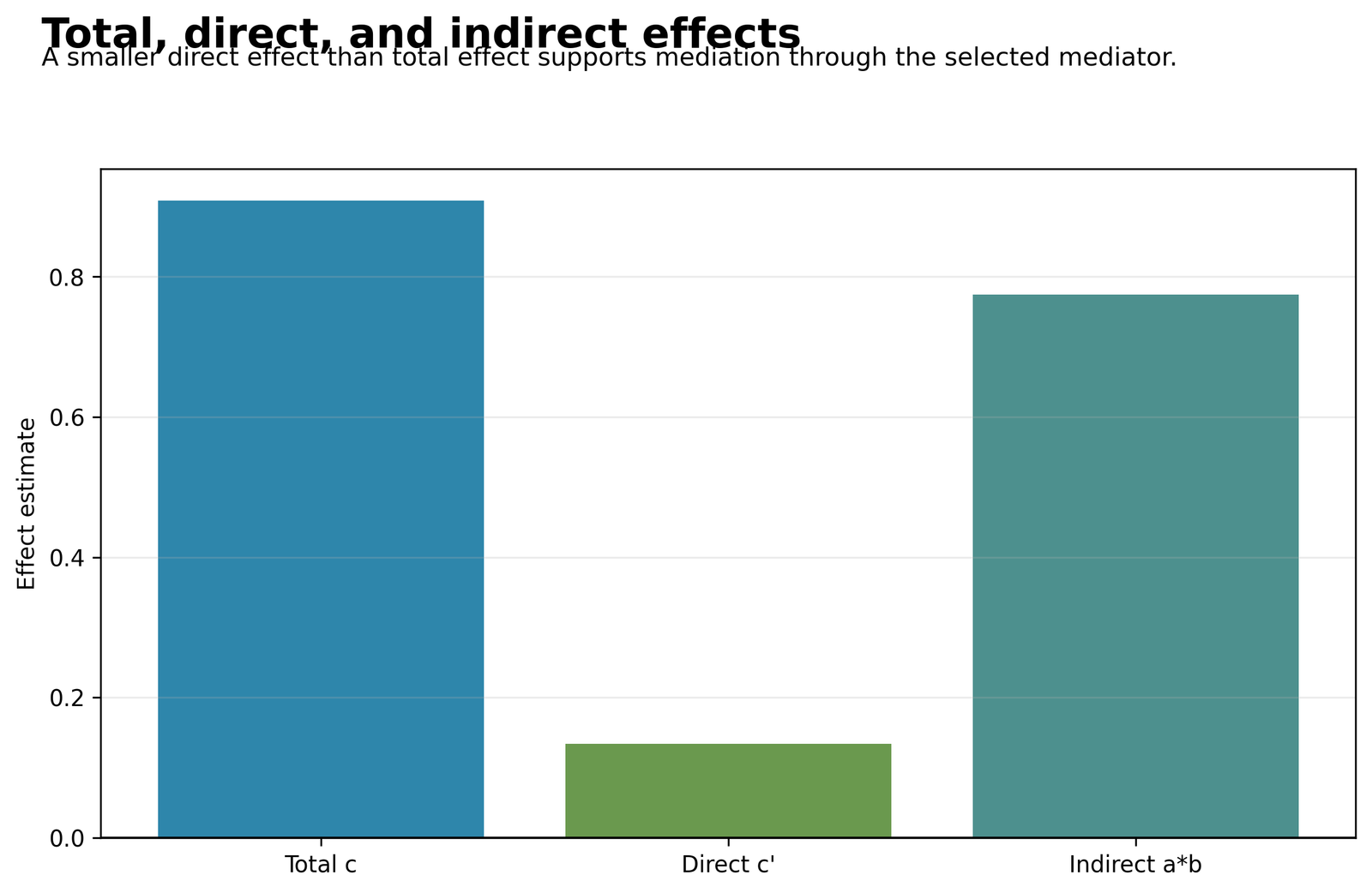
R Chart 4: Mediated Regression Effect Decomposition
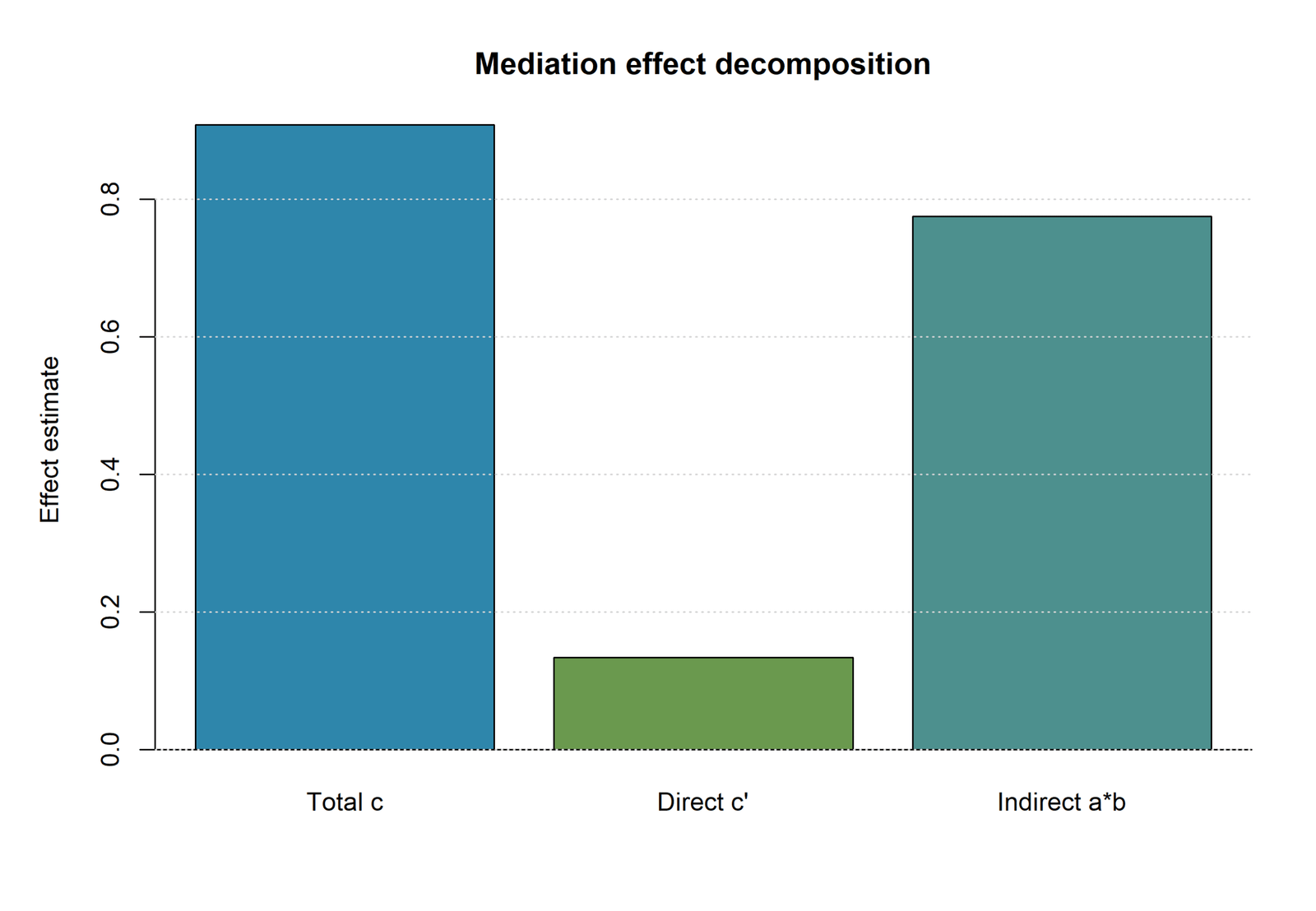
The bars compare the total G1 effect, the direct effect after adding G2, and the product-of-coefficients indirect effect.
Total effect c = 0.908578; direct effect c′ = 0.133732; indirect effect a×b = 0.774846. The decomposition satisfies c ≈ c′ + a×b.
Approximately 85.28% of the total association is represented by the indirect pathway. The proportion is descriptive and should be interpreted carefully when effects have different signs or when the total effect is close to zero.
Report unstandardized effects, bootstrap uncertainty and the remaining direct effect. Avoid using the proportion as a universal causal percentage.
R Chart 5: Bootstrap Indirect-Effect Distribution
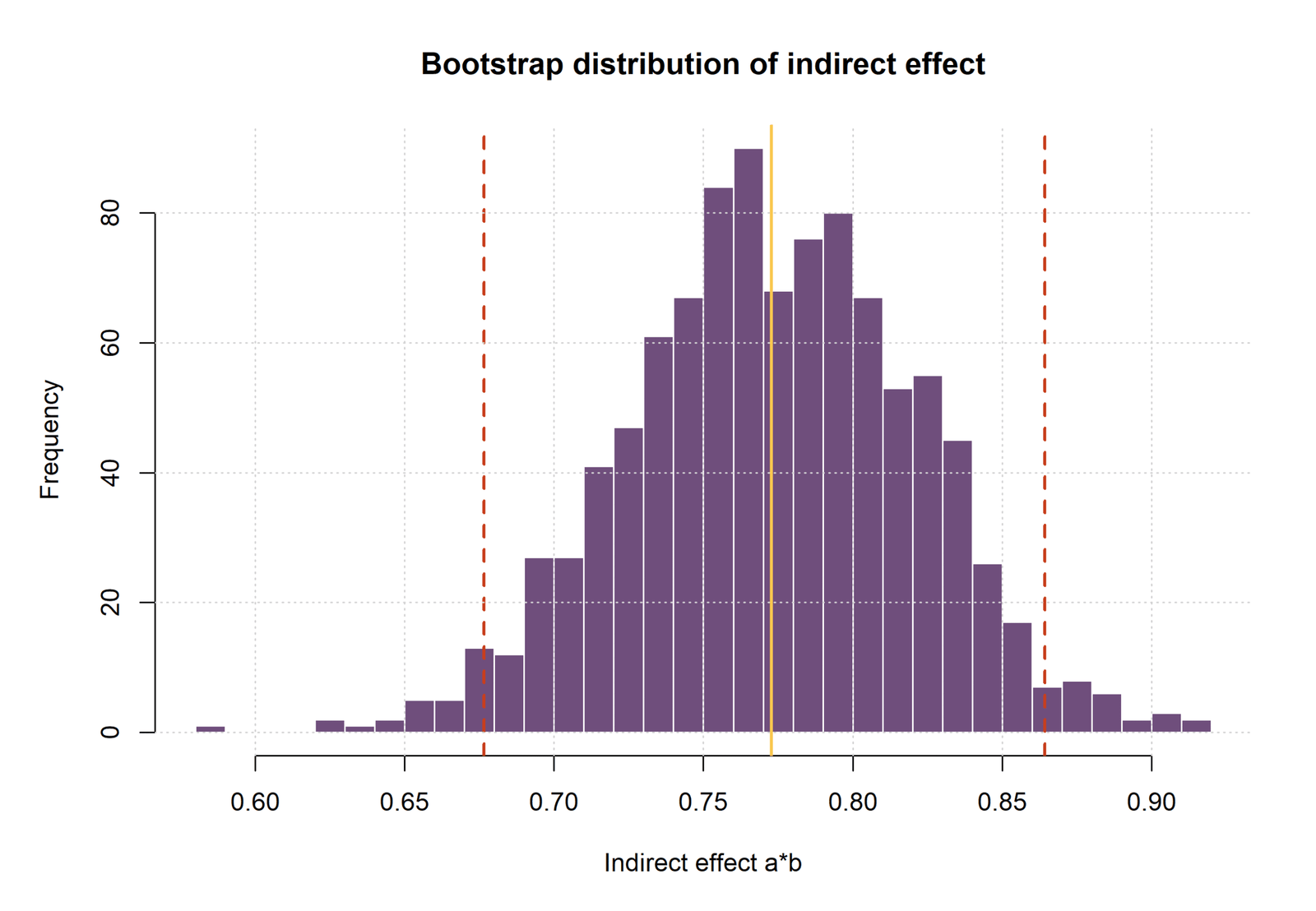
The histogram shows the empirical sampling distribution of a×b created by repeatedly resampling the 649 observations and refitting both regression equations.
Observed indirect effect = 0.774846; R bootstrap mean = 0.772725; bootstrap SD = 0.048042; R 95% percentile CI = [0.676560, 0.864288].
The entire percentile interval is above zero, so the indirect effect is supported. Bootstrap inference is preferred because the product a×b is not generally normally distributed.
State the number of successful resamples, interval method and sampling unit. Use cluster-aware resampling when observations are nested.
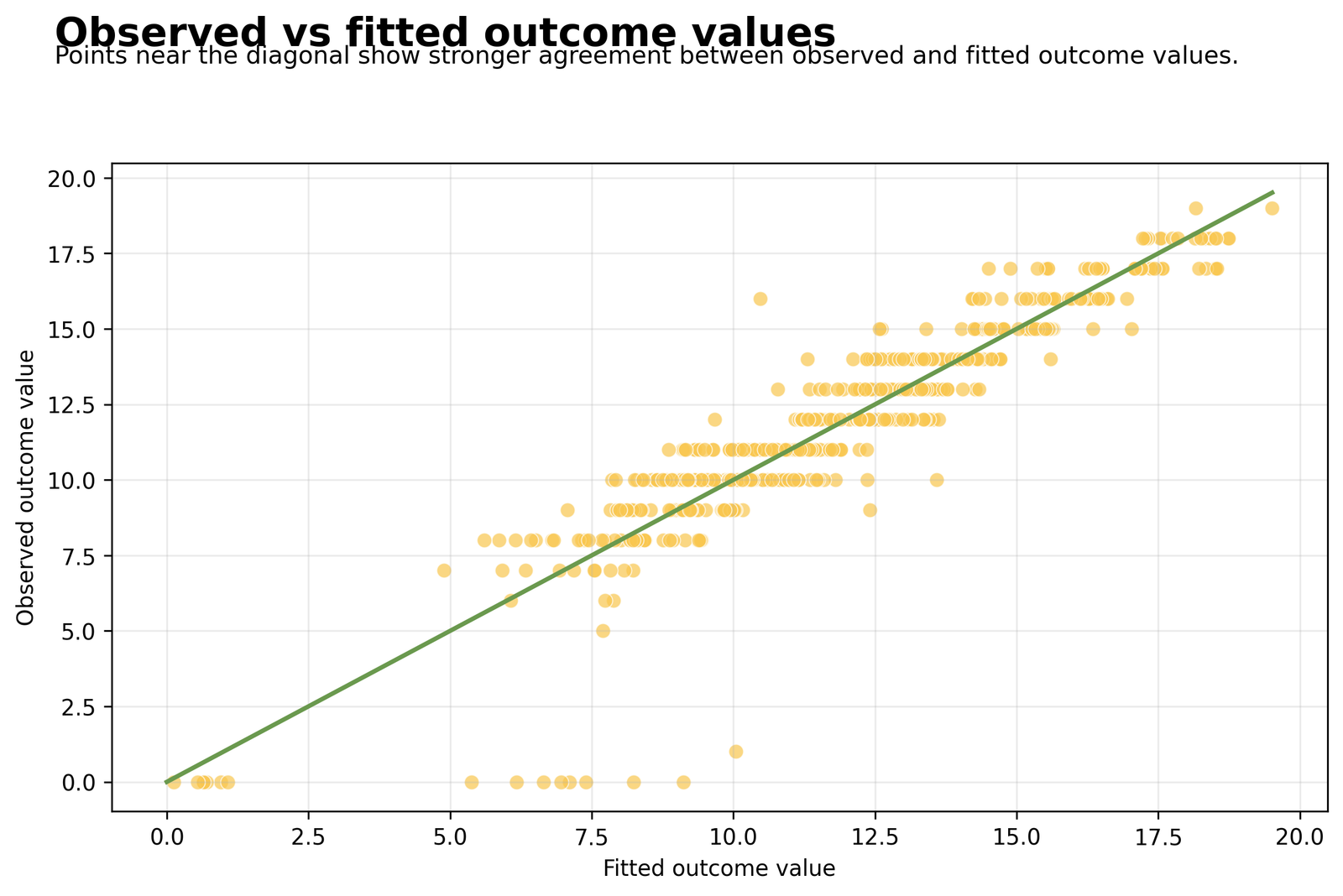
R Chart 6: Observed vs Fitted G3
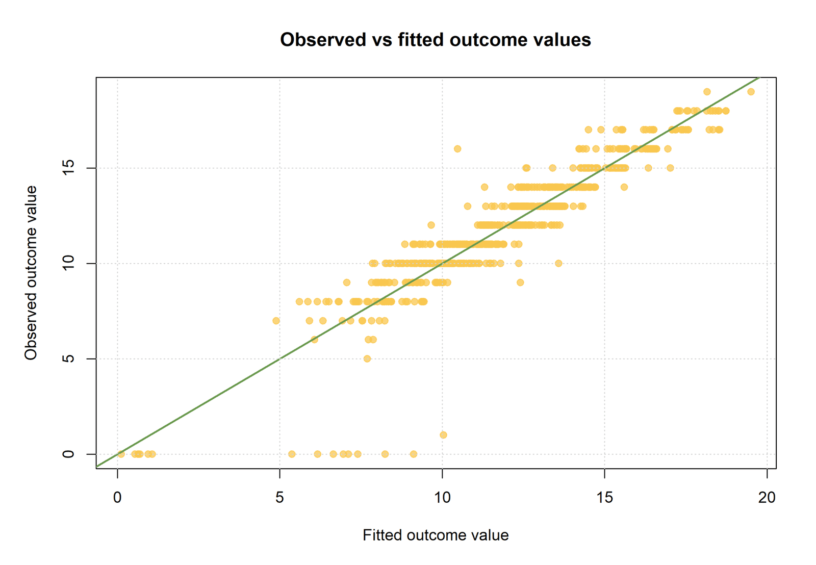
The plot compares observed final grades with predictions from the outcome equation containing G1, G2 and all covariates.
Outcome-model R² = 0.8524, adjusted R² = 0.8501. Most fitted values follow the agreement line through the central grade range, while some observed zeros receive substantially higher predictions.
The model fits the dominant grade pattern well, but high explained variance does not eliminate individual prediction errors. G2 creates the major increase in fit relative to the total-effect model R² of 0.6991.
Review fitted error, calibration and unusual low-grade cases. Prediction performance is not the same question as indirect-effect inference.
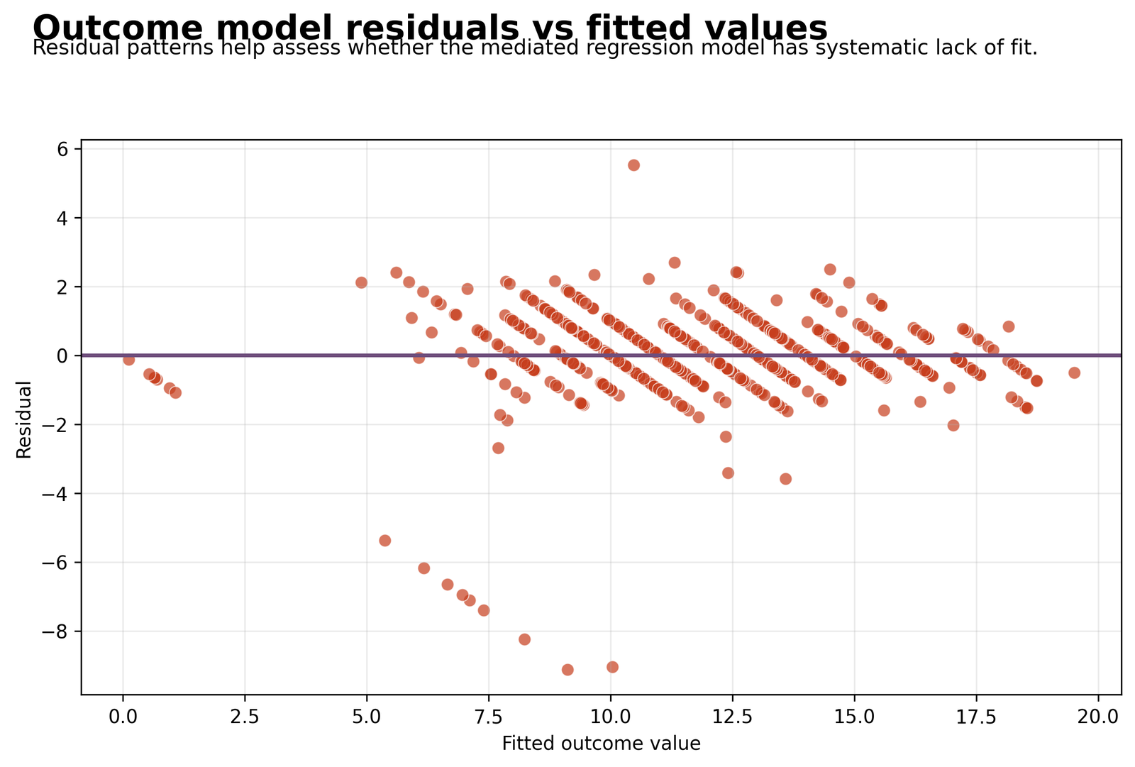
R Chart 7: Outcome Residuals vs Fitted Values
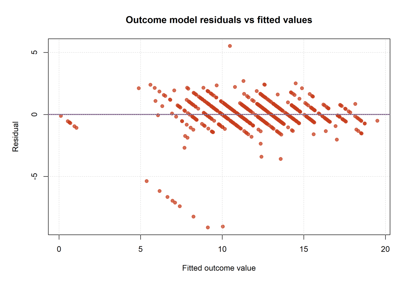
Residuals equal observed G3 minus fitted G3. The chart checks centering, nonlinear patterns, changing variance and extreme observations.
Most residuals cluster near zero and within approximately two grade points. A small number of negative residuals extend much farther because observed G3 is zero or very low while fitted G3 is moderate.
The central linear pattern is strong, but the long negative tail can affect normality and influence. The residual structure should be reported even though the indirect-effect interval is clearly positive.
Use studentized residuals, leverage, Cook’s distance and robust or bootstrap sensitivity analyses. Confirm that extreme observations are genuine before considering exclusions.
Python Mediated Regression Charts in Paired Validation Layout
Why the Python charts are shown second: they confirm the same story with a separate software workflow. The left chart and left explanation belong together, and the right chart and right explanation belong together.
After the R charts are explained in full, the Python charts appear two at a time. Two aligned explanation boxes sit directly underneath in the same left-to-right order, and the mobile layout stacks each chart with its correct explanation.
Mediated Regression is therefore supported by the same effect decomposition in both software workflows.
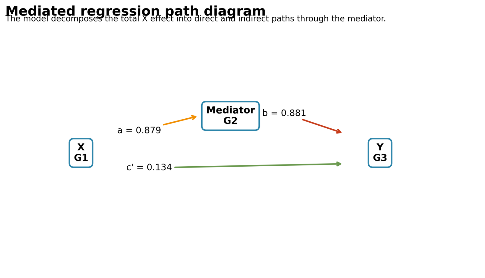
Python Chart 1: Mediated Regression Path Diagram
a = 0.879067, b = 0.881441, c = 0.908578, c′ = 0.133732, a×b = 0.774846.
Python Chart 2: Path a Predictor-to-Mediator Relationship
Path a has SE 0.024436, t 35.9740, p approximately 9.61×10⁻156, CI [0.831082, 0.927052].
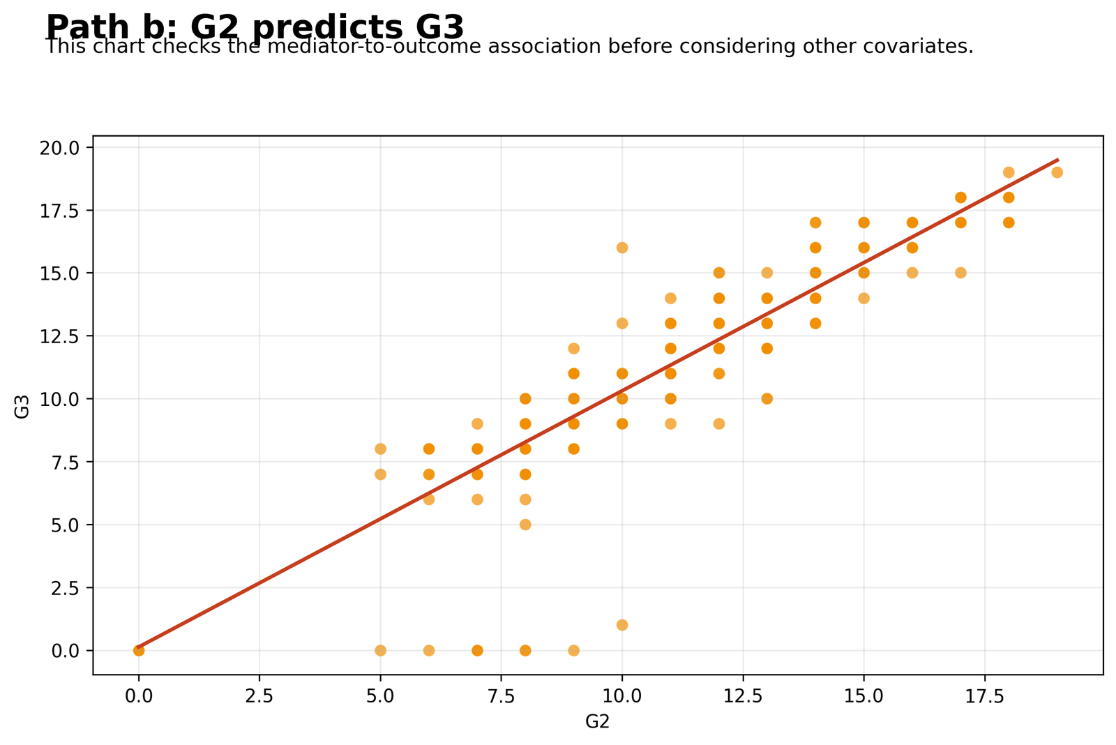
Python Chart 3: Path b Mediator-to-Outcome Relationship
b = 0.881441; direct-and-mediator outcome R² = 0.852375, adjusted R² = 0.850061.
Python Chart 4: Effect Decomposition
c = 0.908578, c′ = 0.133732, a×b = 0.774846, proportion mediated = 0.852811.
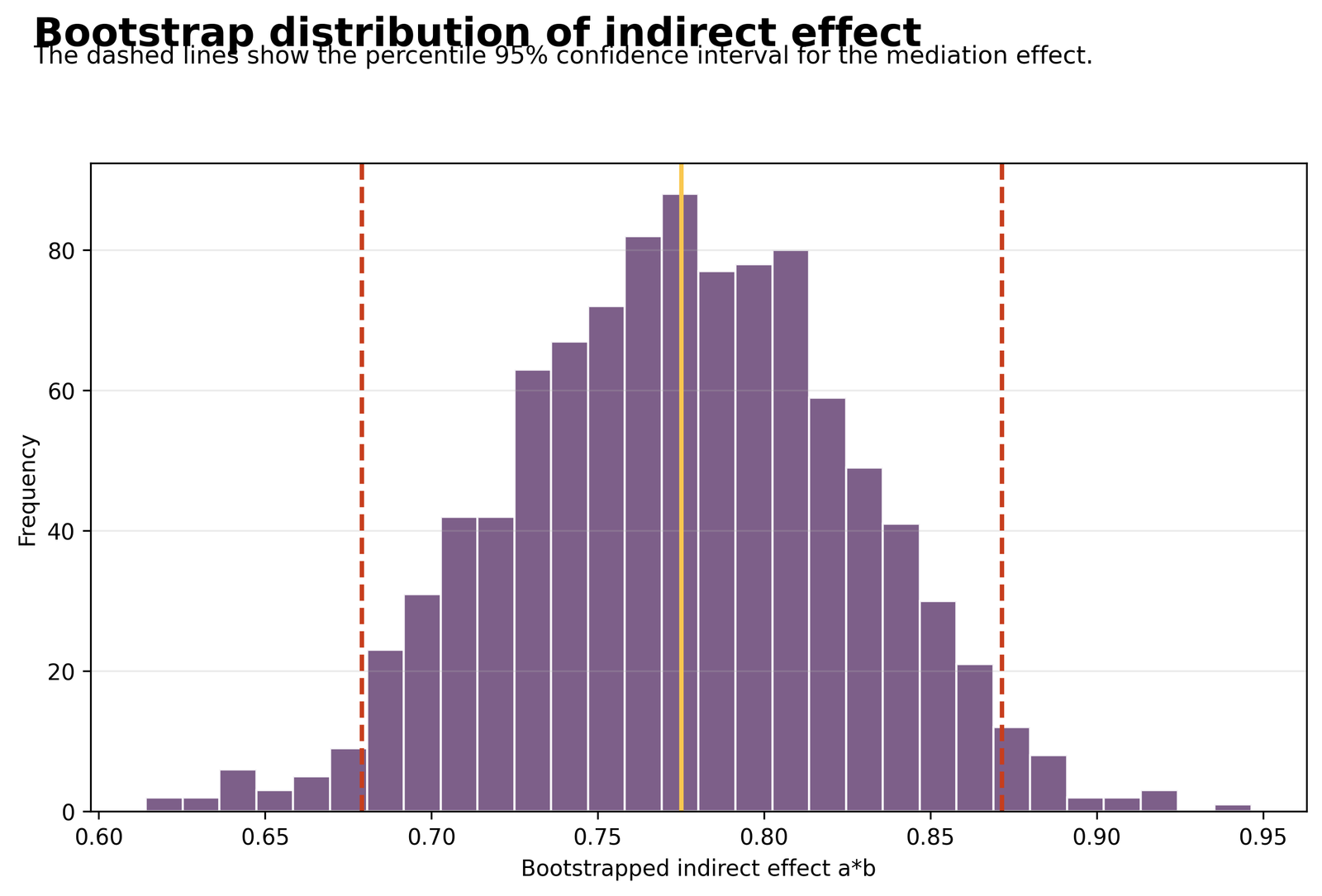
Python Chart 5: Bootstrap Indirect-Effect Distribution
Bootstrap mean = 0.7752, SD = 0.0512, 95% CI = [0.679190, 0.871526].
Python Chart 6: Observed vs Fitted Outcome
The outcome model explains 85.24% of G3 variance, compared with 69.91% in the total-effect model.
Bootstrap 95% confidence intervals
Python Chart 7: Residuals vs Fitted Values
Most residuals are modest, while several low observed G3 cases fall far below their fitted values.
Python Chart 8: Bootstrap Interval Cross-Check
Python CI = [0.679190, 0.871526]; R CI = [0.676560, 0.864288]; observed a×b = 0.774846.
Mediated Regression in SPSS: Model and Coefficient Cross-Checks
The SPSS output fits the same G1 → G2 → G3 structure but includes higher-education intention and internet access in addition to studytime, failures, age, absences, school, sex and address. This expanded specification produces coefficients that are close to the Python and R results.
SPSS path and total models
- Path a B = 0.877, SE = 0.025, p < .001
- Path-a model R² = 0.757
- Total effect c = 0.899, SE = 0.030, p < .001
- Total-model R² = 0.701
SPSS direct and mediator model
- Direct effect c′ = 0.130, SE = 0.037, p < .001
- Path b = 0.877, SE = 0.034, p < .001
- Outcome-model R² = 0.852
- Approximate product a×b = 0.769
The SPSS outcome equation also finds failures negative, B = -0.213, p = .027. The sex contrast is borderline at p = .050, while studytime, age, absences, school, address, higher-education intention and internet access are not statistically significant in the complete equation.
SPSS regression tables provide a useful coefficient and fit cross-check, but the bootstrap product interval from Python and R remains the principal evidence for the indirect effect. A manual product estimate or a change from c to c′ is not a substitute for bootstrap uncertainty.
Mediated Regression Assumptions and Diagnostics
Beginner idea: a result can be statistically significant and still come from a poorly fitted model. Diagnostics check whether the regression equations behave reasonably and whether a few unusual observations are controlling the conclusion.
Check the regression equations
- Linearity: the average relationship should be reasonably straight unless nonlinear terms are added.
- Residual spread: errors should not become much wider as fitted values increase.
- Influence: one or two cases should not determine the path coefficients.
- Multicollinearity: predictors should not be so strongly related that the slopes become unstable.
Check the mediation logic
- G1 should occur before G2, and G2 should occur before G3.
- Important confounders of G1–G2 and G2–G3 should be considered.
- The mediator and outcome should be measured reliably.
- The bootstrap should resample the correct independent unit.
Residual checks
Residuals are the differences between observed and predicted values. Large residuals mean the model predicted a case poorly. Start with Studentized Residuals, then use Cook’s Distance and Influence Diagnostics to identify observations that may strongly affect the fitted paths.
For unusual combinations of several predictors, use Mahalanobis Distance. For a general introduction, see Outlier Detection.
Residual variance checks
If residual spread changes across fitted values, classical standard errors may be inaccurate. The Breusch-Pagan Test and White Test are useful checks for heteroskedasticity.
Normality checks
The raw grades do not need to be perfectly normal. What matters more is whether the residual distribution is reasonable for the inference being used. Review a Q-Q Plot, a P-P Plot, and the Shapiro-Wilk Test. The Skewness and Kurtosis guide explains how shape statistics should be interpreted.
Multicollinearity checks
G1 and G2 are strongly related, which is expected, but the relationship can make the direct and mediator slopes less stable. Use the Multicollinearity Check, Variance Inflation Factor, and Tolerance Statistic guides.
Mediated Regression in Python, R, SPSS and Excel
Python Mediated Regression
New Python users can first review Correlation in Python to understand data loading, variables and basic statistical output.
Fit three statsmodels OLS equations, extract a, b, c and c′, and bootstrap rows to estimate the percentile interval for a×b.
- 1,000 bootstrap samples
- Exact path-coefficient tables
- Model-fit tables
- Seven charts
R Mediated Regression
New R users can first review Correlation in R before working with multiple linked regression equations.
Fit equivalent lm equations, resample row indices, calculate a×b in every successful sample and report the percentile endpoints.
- Independent bootstrap replication
- Same core specification
- Path and fit verification
- Seven chart outputs
SPSS Mediated Regression
New SPSS users can first review Correlation in SPSS to understand variable selection, output tables and significance columns.
Fit the mediator, total-effect and direct-plus-mediator equations with linear regression. Use PROCESS or a compatible bootstrap routine when available for the indirect-effect interval.
- Model summaries and ANOVA
- Coefficients and confidence intervals
- Collinearity diagnostics
- Distribution and residual outputs
Excel Mediated Regression
New Excel users can first review Correlation in Excel to understand worksheet ranges, formulas and interpretation.
Use the workbook to organize path coefficients, calculate a×b, the proportion mediated and Sobel quantities, and document bootstrap endpoints exported from Python or R.
- Data template
- Path-coefficient sheet
- Mediation-effects formulas
- Bootstrap and report templates
Mediated Regression Excel Formulas and Workbook Structure
The worked workbook separates data preparation, path coefficients, effect calculations, bootstrap values and reporting. The Path_Coefficients sheet stores a, b, c and c′ with their standard errors. The Mediation_Effects sheet links those values and calculates the indirect effect, proportion mediated, Sobel standard error and final bootstrap decision.
For the exact analysis, the product is 0.879067 × 0.881441 = approximately 0.774846. The proportion is 0.774846 ÷ 0.908578 = approximately 0.852811. The workbook should record the bootstrap endpoints from the analytical software because a small demonstration list is not a replacement for the complete 1,000-sample distribution.
The Bootstrap_CI sheet can store one row per resample, including the estimated a path, b path, product and direct effect. The 2.5th and 97.5th percentiles become the percentile confidence interval. The Report_Template sheet then converts the values into a structured narrative.
Mediated Regression Code: Expand the Software You Need
Python Mediated Regression and bootstrap code
import numpy as np
import pandas as pd
import statsmodels.formula.api as smf

df = pd.read_csv("dataset.csv")

mediator_formula = (
    "G2 ~ G1 + studytime + failures + absences + age + Medu"
    " + C(school) + C(sex) + C(address)"
)
total_formula = (
    "G3 ~ G1 + studytime + failures + absences + age + Medu"
    " + C(school) + C(sex) + C(address)"
)
outcome_formula = (
    "G3 ~ G1 + G2 + studytime + failures + absences + age + Medu"
    " + C(school) + C(sex) + C(address)"
)

m_a = smf.ols(mediator_formula, data=df).fit()
m_total = smf.ols(total_formula, data=df).fit()
m_outcome = smf.ols(outcome_formula, data=df).fit()

a = m_a.params["G1"]
b = m_outcome.params["G2"]
c = m_total.params["G1"]
c_prime = m_outcome.params["G1"]
indirect = a * b

rng = np.random.default_rng(42)
boot = []

for _ in range(1000):
    indices = rng.integers(0, len(df), len(df))
    sample = df.iloc[indices].copy()
    try:
        a_star = smf.ols(mediator_formula, data=sample).fit().params["G1"]
        b_star = smf.ols(outcome_formula, data=sample).fit().params["G2"]
        boot.append(a_star * b_star)
    except Exception:
        continue

lower, upper = np.percentile(boot, [2.5, 97.5])

print(a, b, c, c_prime, indirect)
print(lower, upper)
R Mediated Regression and bootstrap code
df <- read.csv("dataset.csv", stringsAsFactors = TRUE)

mediator_formula <- G2 ~ G1 + studytime + failures +
  absences + age + Medu + school + sex + address

total_formula <- G3 ~ G1 + studytime + failures +
  absences + age + Medu + school + sex + address

outcome_formula <- G3 ~ G1 + G2 + studytime + failures +
  absences + age + Medu + school + sex + address

m_a <- lm(mediator_formula, data = df)
m_total <- lm(total_formula, data = df)
m_outcome <- lm(outcome_formula, data = df)

a <- coef(m_a)[["G1"]]
b <- coef(m_outcome)[["G2"]]
c_total <- coef(m_total)[["G1"]]
c_prime <- coef(m_outcome)[["G1"]]
indirect <- a * b

set.seed(42)
boot_indirect <- replicate(1000, {
  ids <- sample(seq_len(nrow(df)), replace = TRUE)
  d <- df[ids, ]
  a_star <- coef(lm(mediator_formula, data = d))[["G1"]]
  b_star <- coef(lm(outcome_formula, data = d))[["G2"]]
  a_star * b_star
})

quantile(boot_indirect, c(.025, .975), na.rm = TRUE)
SPSS regression-equation syntax
* Path a: mediator model.
REGRESSION
 /DEPENDENT G2
 /METHOD=ENTER G1 studytime failures age absences
   school_MS sex_M address_U higher_yes internet_yes
 /STATISTICS COEFF OUTS R ANOVA CI(95) COLLIN TOL.

* Total-effect model.
REGRESSION
 /DEPENDENT G3
 /METHOD=ENTER G1 studytime failures age absences
   school_MS sex_M address_U higher_yes internet_yes
 /STATISTICS COEFF OUTS R ANOVA CI(95) COLLIN TOL.

* Direct and mediator outcome model.
REGRESSION
 /DEPENDENT G3
 /METHOD=ENTER G1 G2 studytime failures age absences
   school_MS sex_M address_U higher_yes internet_yes
 /STATISTICS COEFF OUTS R ANOVA CI(95) COLLIN TOL
 /SAVE PRED RESID ZPRED ZRESID COOK LEVER.

OUTPUT SAVE
 /OUTFILE='D:\DATA ANALYSIS\H Regression Tests and Models\Mediated Regression\SPSS_Output\spv\Mediated-Regression.spv'.

OUTPUT EXPORT
 /CONTENTS EXPORT=ALL LAYERS=PRINTSETTING MODELVIEWS=PRINTSETTING
 /PDF DOCUMENTFILE='D:\DATA ANALYSIS\H Regression Tests and Models\Mediated Regression\SPSS_Output\pdf\Mediated-Regression-SPSS-Output.pdf'.
Excel effect formulas
Indirect effect:
=Path_A_Cell*Path_B_Cell

Proportion mediated:
=Indirect_Effect_Cell/Total_Effect_Cell

Sobel standard error:
=SQRT((Path_B^2*SE_A^2)+(Path_A^2*SE_B^2))

Sobel z:
=Indirect_Effect/Sobel_SE

Bootstrap CI lower:
=PERCENTILE.INC(Bootstrap_Indirect_Range,0.025)

Bootstrap CI upper:
=PERCENTILE.INC(Bootstrap_Indirect_Range,0.975)

Decision:
=IF(OR(CI_Lower>0,CI_Upper<0),
 "Indirect effect supported",
 "Interval includes zero")
How a New Student Should Study This Mediated Regression Example
- Identify X, M and Y: G1 is X, G2 is M and G3 is Y.
- Read the path diagram: follow G1 → G2 → G3, then notice the remaining G1 → G3 arrow.
- Learn paths a and b: these two paths create the indirect effect.
- Compare c and c′: the G1 coefficient becomes much smaller after G2 enters.
- Read the bootstrap interval: both limits are above zero, so the indirect effect is supported.
- Check diagnostics: strong statistical evidence does not remove the need to examine residuals and influential cases.
- Write the conclusion carefully: describe a supported indirect association unless the design justifies causal language.
Before moving to advanced material, make sure you can explain the model without symbols: earlier grade predicts middle grade, middle grade predicts final grade, and most of the earlier-to-final relationship is represented by the middle grade.
For broader foundations, review Descriptive Statistics, Histogram Interpretation, and Normal Distribution.
Advanced Mediated Regression Interpretation and Extensions
The main reading path remains compact. Expand only the technical topics needed for the study.
Students planning a new study should also review Statistical Power and Effect Size. Power concerns whether the sample is large enough to detect the indirect effect, while effect size concerns the practical magnitude of the pathway.
Mediated Regression versus path analysis
- A single observed-variable mediator can be estimated with ordinary regression equations.
- Path analysis generalizes the structure to several simultaneous observed pathways.
- Structural equation modeling adds latent variables, measurement models and global fit.
Mediated Regression versus moderation
- Mediation asks how or through what variable an association operates.
- Moderation asks when, for whom or at what level an association changes.
- Moderated mediation combines the two questions through conditional indirect effects.
Why c approximately equals c-prime plus a times b
- The decomposition holds for the same linear sample and compatible covariate specification.
- The reported values sum to 0.908578 after rounding.
- Different links, scales or samples can break the simple equality.
Interpreting the residual model improvement
- Adding G2 raises outcome R² from 0.6991 to 0.8524.
- The increase reflects the strong conditional predictive contribution of G2.
- The fit increase supports the pathway description but is not itself the indirect-effect test.
Why independent bootstrap replications are valuable
- Python and R independently resample rows and refit both equations.
- Their intervals overlap strongly despite different random draws.
- Independent replication reduces concern that one software implementation or seed drives the decision.
How to report near-zero p-values
- Write p < .001 rather than p = .000.
- R may display scientific notation for extremely small probabilities.
- The confidence interval and effect magnitude remain more informative than a very small p-value alone.
Why raw-variable normality tests reject
- Large samples make formal tests sensitive to minor departures.
- Bounded integer grades are not expected to be perfectly normal.
- Focus on residual behavior, model form and bootstrap robustness.
Counterfactual interpretation
- A causal indirect effect compares potential mediator and outcome values under different exposures.
- Regression products equal causal effects only under identification assumptions.
- Observational results should use cautious language unless those assumptions are defended.
Mediator-outcome confounding affected by X
- A variable caused by X that also affects M and Y creates a difficult post-treatment confounding problem.
- Simply controlling it can introduce bias.
- Study design and causal diagrams should guide adjustment.
Sequential ignorability
- One assumption concerns exposure assignment given baseline covariates.
- A second concerns mediator assignment given exposure and covariates.
- These assumptions are strong and cannot be verified solely from the observed regression tables.
Cluster bootstrap
- When students are sampled within schools, resampling individual rows may understate uncertainty.
- A cluster bootstrap resamples schools and retains students within selected schools.
- The appropriate resampling unit follows the independent sampling unit.
Monte Carlo confidence intervals
- An alternative simulates a and b from their estimated joint distribution.
- The product is calculated in every simulation.
- Bootstrap intervals remain more direct when row-level data and computing resources are available.
Joint significance approach
- The joint-significance approach requires significant a and b paths.
- It has reasonable power but does not directly produce an interval for a×b.
- Use the bootstrap product interval as the main result.
Suppression and inconsistent mediation
- Direct and indirect effects can have opposite signs.
- The total effect may then be smaller than either component or close to zero.
- Proportion-mediated ratios are inappropriate in inconsistent mediation.
Effect scaling
- All focal grades use the same 0–19 scale, making unstandardized coefficients especially interpretable.
- One G1 point predicts about 0.879 G2 points, and one G2 point predicts about 0.881 G3 points conditional on G1.
- The indirect product is expressed in G3 points per one G1 point.
Robust standard errors
- Heteroskedasticity-consistent standard errors can be applied to each regression equation.
- A bootstrap that refits the equations can also reflect some non-normal sampling behavior.
- Use both as sensitivity analyses when residual variance changes substantially.
Nonlinear mediated pathways
- A linear product can miss threshold, ceiling or curved relationships.
- Polynomial or spline terms may be included with careful effect definition.
- The indirect effect can become conditional on the value of X.
Interaction between X and mediator
- If G1 changes the effect of G2 on G3, the indirect effect varies with G1.
- The outcome equation must include the G1×G2 interaction.
- Report conditional indirect effects rather than one constant product.
Measurement timing in the student example
- G1 precedes G2 and G2 precedes G3 in the school-year sequence.
- This temporal order is stronger than measuring all three simultaneously.
- Unmeasured academic ability, motivation and classroom factors can still confound the pathways.
Practical meaning of the remaining direct effect
- The direct coefficient 0.1337 represents the adjusted G1–G3 association not represented by the included G2 pathway.
- It can reflect other mechanisms, measurement overlap or omitted mediators.
- It should not be interpreted as a single known direct process.
Why the indirect effect is a product
- Path a converts a one-unit X difference into an expected M difference.
- Path b converts a one-unit M difference into an expected Y difference while X is controlled.
- Multiplying the two coefficients places the pathway on the Y scale per one-unit X difference.
Why bootstrap inference is preferred
- The product of two approximately normal coefficients is not generally normal.
- Percentile resampling estimates the empirical shape without relying on a symmetric Sobel interval.
- Report the resampling unit, number of successful samples and interval method.
Partial versus complete mediation
- The direct effect remains positive and significant in this analysis.
- The term partial mediation describes coexistence of indirect and direct components.
- Avoid treating a non-significant direct effect as proof that no direct pathway exists.
Why the total effect need not be significant first
- A positive and negative pathway can cancel in the total effect.
- Modern indirect-effect testing does not require a significant c path as a preliminary gate.
- Theory and bootstrap evidence should guide the pathway conclusion.
Interpreting the proportion mediated
- The ratio is about 0.8528 in this analysis.
- It is most stable when direct and indirect effects have the same sign.
- It should not be interpreted as a literal causal percentage without stronger assumptions.
Unstandardized versus standardized effects
- Unstandardized effects retain grade-point units and satisfy the simple c = c′ + a×b decomposition.
- Standardized effects depend on variable variances and may not decompose identically under every convention.
- Use unstandardized bootstrap effects as the primary report.
Covariate selection
- Include variables that confound focal paths rather than every available variable automatically.
- Post-treatment covariates can distort the mediated pathway.
- State why each covariate belongs in the mediator and outcome equations.
Temporal ordering
- A defensible sequence requires G1 before G2 before G3 in time.
- Temporal order strengthens interpretation but does not remove all confounding.
- Repeated measurement designs are stronger than one-time cross-sectional data.
Mediator measurement reliability
- Measurement error in G2 can attenuate path b and distort the indirect effect.
- Reliability should be reported for latent or multi-item mediators.
- Structural equation modeling can represent measurement error explicitly.
Multiple mediators
- Parallel mediators estimate several indirect effects without ordering the mediators.
- Serial mediators impose an ordered chain.
- Shared mediator variance makes individual indirect effects conditional on the other mediators.
Moderated mediation
- A pathway may vary across levels of another variable.
- Conditional indirect effects require interaction terms in path a, path b or both.
- Report index-of-moderated-mediation intervals rather than separate subgroup significance claims.
Categorical mediators or outcomes
- Binary or count variables require generalized models rather than ordinary Gaussian equations.
- Products from nonlinear models need scale-aware interpretation.
- Natural-effect or simulation approaches may be preferable for causal interpretation.
Multilevel mediated regression
- Students nested within schools can violate independence.
- Within-school and between-school indirect effects are different quantities.
- Use multilevel mediation when the sampling and pathway structure are clustered.
Longitudinal mediated regression
- Measure X before M and M before Y when possible.
- Control prior levels of M and Y to distinguish change from stable differences.
- Cross-lagged or latent-change models can address more complex temporal processes.
Sensitivity to unmeasured confounding
- A positive bootstrap interval does not test the no-unmeasured-confounding assumptions.
- Sensitivity analysis can quantify how strong an omitted confounder would need to be.
- State this limitation explicitly in observational research.
Linearity and functional form
- Each equation assumes a linear conditional mean unless nonlinear terms are added.
- Grade ceiling and floor effects may create curvature.
- Use partial-residual plots, polynomial terms or splines when justified.
Homoscedasticity
- Constant residual variance supports classical standard errors in each equation.
- Bootstrap inference for a×b does not automatically fix every model misspecification.
- Review residual plots and robust-standard-error sensitivity.
Multicollinearity between G1 and G2
- The strong a path implies substantial shared variation.
- Path b and c′ remain conditional coefficients in the presence of that overlap.
- Report VIF or tolerance and avoid interpreting c′ as a simple G1–G3 association.
Influential observations
- An observation can affect a, b or both and therefore have a multiplied effect on a×b.
- Inspect influence in both equations.
- Bootstrap distributions may reveal instability when influential cases are repeatedly selected.
Missing data
- All equations should use the same analysis sample.
- Listwise deletion can change the target population and reduce precision.
- Multiple imputation should preserve the mediation structure and combine indirect effects appropriately.
Bootstrap sample size
- One thousand samples provide a useful worked analysis.
- Five thousand or more may stabilize tail percentiles for publication.
- More resamples reduce Monte Carlo error but do not correct model bias.
Percentile versus bias-corrected intervals
- This analysis reports percentile endpoints.
- Bias-corrected methods adjust for bias and acceleration but may behave differently in small samples.
- Name the interval method so results can be reproduced.
Sobel test limitations
- The Sobel test uses a normal approximation for a×b.
- It can be conservative or inaccurate when the product distribution is asymmetric.
- Use it as a supplementary calculation rather than the primary decision.
Prediction versus pathway explanation
- The outcome model R² increases strongly when G2 enters.
- High prediction fit does not by itself prove the proposed mechanism.
- Pathway claims require theory, timing and confounding control in addition to fit.
Comparing Python and R bootstrap intervals
- The Python lower and upper limits are 0.6792 and 0.8715.
- The R limits are 0.6766 and 0.8643.
- The small difference is consistent with independent random resamples and both intervals support the same decision.
Comparing SPSS with Python and R
- SPSS adds higher and internet covariates, while Python and R use Medu.
- The rounded SPSS paths remain close: a ≈ 0.877, b ≈ 0.877, c ≈ 0.899 and c′ ≈ 0.130.
- Compare scientific conclusions rather than demanding identical numbers from different specifications.
AIC and BIC differences across software
- Python and R show identical fitted coefficients and R² but AIC/BIC differ by small constants.
- Software can define likelihood constants and parameter counts differently.
- Compare information criteria within one software implementation and identical data specification.
Effect decomposition check
- The observed values satisfy 0.133732 + 0.774846 ≈ 0.908578.
- This arithmetic check helps identify coding or extraction errors.
- Rounding can create tiny discrepancies.
Statistical power for indirect effects
- Power depends on both a and b, their uncertainty and sample size.
- A weak link can make the product difficult to detect even when the other path is strong.
- Simulation-based planning is more informative than planning from one coefficient alone.
Causal language
- Use ‘indirect association’ or ‘statistically supported indirect effect’ for observational designs.
- Use causal terms only with appropriate identification assumptions and design.
- Distinguish statistical mediation from a proven mechanism.
Reproducibility
- Save formulas, covariate lists, factor references, seed and bootstrap indices.
- Export the complete path and model-fit tables.
- Regenerate charts and reports directly from code.
APA-Style Reporting for Mediated Regression
Mediated Regression Publication Checklist and Common Mistakes
Report these items
- X, mediator and outcome with measurement timing
- All covariates and categorical references
- Path a, path b, total c and direct c′
- Indirect effect a×b
- Bootstrap sample count and interval method
- Bootstrap confidence interval and decision
- Proportion mediated with caution
- Model R² and residual diagnostics
- Software-specific specification differences
- Design and causal limitations
Avoid these mistakes
- Requiring a significant total effect before testing a×b
- Calling mediation supported only because a and b are significant
- Using c−c′ without uncertainty as the final test
- Reporting a Sobel p-value instead of bootstrap evidence
- Mixing standardized and unstandardized effects
- Changing covariates across equations without explanation
- Ignoring temporal order and confounding assumptions
- Interpreting the proportion as a proven causal percentage
- Deleting outliers only to improve significance
- Claiming identical software results from different models
Mediated Regression Downloads
R Mediated Regression ReportIndependent path replication, bootstrap CI and seven charts.
SPSS Mediated Regression OutputRegression equations, coefficients, model summaries and diagnostics.
Mediated Regression Worked Excel FilePath formulas, effect calculations, bootstrap sheet and report template.
Frequently Asked Questions About Mediated Regression
What is Mediated Regression?
Mediated Regression uses linked regression equations to estimate whether X is associated with Y through a mediator M.
What are X, M and Y in this example?
G1 is X, G2 is the mediator and G3 is the outcome.
How many observations are used?
All 649 observations are used.
What is path a?
Path a is 0.879067 and represents the adjusted G1–G2 association.
What is path b?
Path b is 0.881441 and represents the adjusted G2–G3 association after G1 is controlled.
What is the total effect?
The total G1 effect on G3 is 0.908578.
What is the direct effect?
The remaining direct G1 effect after G2 enters is 0.133732.
What is the indirect effect?
The product a×b is 0.774846.
Is the indirect effect supported?
Yes. Both Python and R bootstrap intervals exclude zero.
What is the Python bootstrap interval?
The Python percentile interval is [0.679190, 0.871526].
What is the R bootstrap interval?
The R percentile interval is [0.676560, 0.864288].
Why are the two intervals different?
They use independent random bootstrap samples and therefore have slightly different endpoints.
How many bootstrap samples were used?
Both reports use 1,000 successful bootstrap samples.
What is the proportion mediated?
The indirect effect divided by the total effect is approximately 0.8528 or 85.28%.
Does 85.28% prove a causal mechanism?
No. It is a descriptive ratio and causal interpretation requires stronger assumptions.
Must the total effect be significant?
No. The indirect effect can be tested directly with a bootstrap interval.
Is a significant path a enough?
No. The indirect product and its uncertainty must be evaluated.
Is a significant path b enough?
No. Mediation concerns the product a×b, not either path alone.
What does a positive direct effect mean?
Some positive G1–G3 association remains after G2 is controlled.
Is this complete mediation?
No. The remaining direct effect is positive and significant, so the pattern includes both direct and indirect components.
Why does SPSS differ slightly?
Its equation includes higher-education intention and internet access, while Python and R use Medu.
What is the SPSS path a coefficient?
The expanded SPSS model reports path a B = 0.877.
What is the SPSS path b coefficient?
The expanded SPSS outcome model reports path b B = 0.877.
Can Excel calculate the indirect effect?
Yes. Multiply path a by path b and import bootstrap endpoints from Python or R.
Should the Sobel test be the main decision?
No. Bootstrap inference is preferred for the asymmetric product distribution.
Can a binary outcome be used?
Yes, but generalized regression and scale-aware indirect-effect methods are required.
Can there be multiple mediators?
Yes. They can be specified in parallel or in a theoretically ordered serial pathway.
Can Mediated Regression establish causation?
Not by itself. Design, timing and confounding assumptions determine causal credibility.
What diagnostics should be checked?
Review linearity, residual variance, influence, multicollinearity and the quality of all focal measurements.
How should the result be reported?
Report X, M, Y, covariates, a, b, c, c′, a×b, bootstrap method, interval and design limitations.
Final Mediated Regression Conclusion
Beginner conclusion: G1 predicts G2, and G2 predicts G3. When G2 is added to the final equation, the G1 coefficient becomes much smaller. This means that G2 explains a large part of the statistical connection between G1 and G3.
Mediated Regression reporting should preserve the exact covariate set because every path is conditional on the variables in its equation.
Mediated Regression does not convert an observational association into a causal mechanism without additional identification assumptions.
Mediated Regression is strongest when theory, temporal order, bootstrap inference and diagnostic evidence point to the same pathway.
Mediated Regression should be interpreted as a linked set of conditional equations rather than as one isolated change in a coefficient.
Mediated Regression reporting should preserve the exact covariate set because every path is conditional on the variables in its equation.
Mediated Regression does not convert an observational association into a causal mechanism without additional identification assumptions.
Mediated Regression is strongest when theory, temporal order, bootstrap inference and diagnostic evidence point to the same pathway.
Mediated Regression should be interpreted as a linked set of conditional equations rather than as one isolated change in a coefficient.
Mediated Regression reporting should preserve the exact covariate set because every path is conditional on the variables in its equation.
Mediated Regression does not convert an observational association into a causal mechanism without additional identification assumptions.
Mediated Regression is strongest when theory, temporal order, bootstrap inference and diagnostic evidence point to the same pathway.
Mediated Regression should be interpreted as a linked set of conditional equations rather than as one isolated change in a coefficient.
Mediated Regression reporting should preserve the exact covariate set because every path is conditional on the variables in its equation.
Mediated Regression does not convert an observational association into a causal mechanism without additional identification assumptions.
Mediated Regression is strongest when theory, temporal order, bootstrap inference and diagnostic evidence point to the same pathway.
Mediated Regression should be interpreted as a linked set of conditional equations rather than as one isolated change in a coefficient.
Mediated Regression identifies a strong pathway from G1 through G2 to G3. Path a is 0.8791 and path b is 0.8814, producing an indirect effect of 0.7748. The total effect is 0.9086, while the direct effect after G2 enters is 0.1337.
The Python and R percentile intervals are entirely positive and overlap closely. Both analyses therefore support the indirect effect. The direct effect remains positive, so the result is best described as a substantial indirect pathway accompanied by a smaller remaining direct association.
SPSS produces closely related coefficients under an expanded covariate specification and confirms the same substantive pattern. The strongest conclusion comes from convergence among path estimates, model fit, bootstrap inference and chart interpretation—not from any single coefficient alone.

