
Ordinary Least Squares Regression: Formula, Interpretation, SPSS, Python, R and Excel Guide
Ordinary Least Squares Regression estimates the relationship between a continuous outcome and one or more predictors by finding the coefficient values that minimize the sum of squared residuals. This guide explains the method before applying it to final grade G3.
Model Overview
Ordinary Least Squares Regression, often shortened to OLS regression, is the standard regression method for a continuous dependent variable. It estimates how the expected value of an outcome changes when one predictor changes while the remaining predictors are held constant. The word ordinary distinguishes the method from weighted or generalized least squares; least squares refers to the rule used to fit the line or plane—the selected coefficients make the squared differences between observed and predicted values as small as possible.
The method answers three related questions. First, does the predictor set collectively explain meaningful variation in the outcome? Second, which predictors contribute unique information after adjustment for the others? Third, how accurately does the fitted equation predict new or existing observations? These questions are addressed through the model F test, R-squared and adjusted R-squared, coefficient tests and confidence intervals, and prediction-error measures such as RMSE and MAE.
Ordinary Least Squares Regression is used when the outcome is quantitative and the relationship with the predictors can be represented adequately by an additive linear equation. The predictors may be numeric, categorical, or a mixture of both. Categorical predictors enter through indicator coding, so their coefficients compare a category with a stated reference group. The method is widely used in education, economics, health research, psychology, business analytics, public policy, engineering, and social science because its coefficients have direct unit-based interpretations.
Why use OLS instead of a simple correlation? A Pearson correlation measures the strength of a two-variable linear association but does not adjust for additional variables. OLS estimates unique adjusted effects and creates a prediction equation. Why use it instead of a group-comparison test? Regression can include several continuous and categorical predictors in one model. Why not use logistic regression? Logistic models are intended for categorical outcomes, whereas OLS is designed for a continuous outcome such as G3.
The fitted equation takes the form Y = β₀ + β₁X₁ + … + βₖXₖ + ε. Each slope coefficient is the expected change in Y for a one-unit increase in that predictor, conditional on the others. The intercept is the expected outcome when all numeric predictors equal zero and all categorical variables are in their reference groups. The residual is the observed value minus the prediction. Squaring residuals prevents positive and negative errors from cancelling and gives larger errors greater influence on the fit.
Good use of Ordinary Least Squares Regression requires more than a high R-squared. The mean relationship should be reasonably linear, residual spread should be reasonably stable, observations should be independent, severe multicollinearity should be absent, and influential cases should be examined. Residual normality matters mainly for small-sample significance tests and confidence intervals; with a large sample, departures should be judged by their magnitude and effect on inference rather than by one normality p-value alone.
OLS differs from Generalized Least Squares Regression because GLS explicitly models unequal variance or correlated errors. It differs from Generalized Estimating Equations and hierarchical models because those methods address clustered or repeated observations. It differs from Generalized Additive Model because GAM can estimate flexible nonlinear functions. OLS remains preferable when the linear specification is adequate, independence is plausible, and readers need direct adjusted mean differences.
In this worked analysis, G3 is the continuous outcome. The Python model uses G1, G2, studytime, failures, absences, age, school, sex, and address. The model explains 85.22% of G3 variation, with adjusted R² of 0.8501, RMSE of 1.2410, and MAE of 0.7799. G2 is the dominant predictor, G1 and failures retain smaller independent effects, and the residual diagnostics reveal strong overall prediction with non-normality concentrated mainly in unusual low outcomes.
Quick Answer
Model result
- F(9,639) = 409.4514
- p < .001
- MAE = 0.7799
Key coefficients
- G2: B = 0.8794
- G1: B = 0.1328
- failures: B = −0.2266
Table of Contents
- What Ordinary Least Squares Regression is
- When and why it is used
- Formula and coefficient meaning
- Variables and coding
- Results at a glance
- Eight chart interpretations
- R chart interpretations
- Coefficient table
- Predictions and errors
- Assumptions and diagnostics
- SPSS, Python, R and Excel
- Code
- Advanced interpretation
- APA-style reporting
- Checklist
- Downloads
- Related guides
- FAQs
What Is Ordinary Least Squares Regression?
Ordinary Least Squares Regression estimates a linear prediction equation for a continuous outcome. The coefficients are selected so that the sum of squared residuals is smaller than it would be under any other set of coefficient values for the same model specification.
The method can be simple, with one predictor, or multiple, with several numeric and categorical predictors. Multiple OLS coefficients are partial effects: each one describes the expected outcome difference associated with its predictor after the other model terms are held constant. This is why partial correlation and semi-partial correlation are closely related concepts.
When and Why Ordinary Least Squares Regression Is Used
Use Ordinary Least Squares Regression when the outcome is continuous, the conditional mean can be represented adequately by a linear equation, and the research question concerns adjusted mean changes or predictions. It is especially useful when several plausible explanations overlap and the goal is to estimate their unique contributions.
The method is not automatically suitable for every numeric-looking outcome. Counts, binary outcomes, bounded proportions, repeated observations, or strongly nonlinear relationships may require another member of the Generalized Linear Model family, Generalized Estimating Equations, Generalized Least Squares Regression, or Generalized Additive Model.
Ordinary Least Squares Regression Formula and Interpretation
A coefficient of 0.8794 for G2 means that two students who differ by one G2 point are expected to differ by about 0.879 G3 points when G1, studytime, failures, absences, age, school, sex, and address are held constant. A coefficient of −0.2266 for failures means one additional prior failure is associated with a 0.227-point lower expected G3 under the same adjustment. This Ordinary Least Squares Regression result should be interpreted with the stated model specification and uncertainty.
Variables Used and Coding
| Variable | Role | Definition | Interpretation |
|---|---|---|---|
| G3 | Outcome | Final grade | Continuous dependent variable |
| G1 | Numeric predictor | First-period grade | Adjusted change per one point |
| G2 | Numeric predictor | Second-period grade | Adjusted change per one point |
| studytime | Numeric predictor | Study-time category | Adjusted mean change |
| failures | Numeric predictor | Previous failures | Adjusted mean change |
| absences | Numeric predictor | School absences | Adjusted mean change |
| age | Numeric predictor | Age in years | Adjusted mean change |
| school | Categorical predictor | GP or MS | MS compared with GP |
| sex | Categorical predictor | F or M | Male compared with female |
| address | Categorical predictor | R or U | Urban compared with rural |
Results at a Glance
Observed-model fit This Ordinary Least Squares Regression result should be interpreted with the stated model specification and uncertainty.
Complexity-adjusted fit
p < .001
Typical squared-error scale
Mean absolute error
9 predictors
Downloads
The Excel workbook uses an expanded 15-predictor specification, so its coefficients should be interpreted as a separate fitted model rather than substituted into the nine-predictor Python results.
Eight Chart Interpretations
Each figure is organized around the visible pattern, the values that define it, the statistical interpretation, and its relevance to the reader.
Chart 1: Outcome Distribution
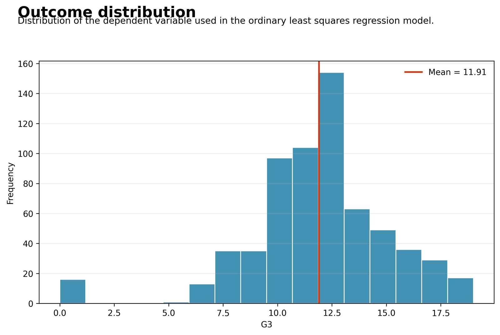
Most G3 values lie in the middle and upper part of the 0–19 scale, with a smaller group of zero outcomes separated from the main cluster.
The sample contains 649 students. G3 has mean about 11.906, standard deviation about 3.231, and range 0–19.
The central mass represents ordinary grade progression, while the zero outcomes create a long lower tail. Those zero cases are likely to produce the largest negative residuals because their G1 and G2 profiles may otherwise resemble students with nonzero final grades.
The model can fit the majority of students well while still failing on a small special subgroup. Distribution shape should therefore be connected to the residual plots rather than treated as a separate descriptive detail.
Chart 2: Observed Versus Predicted G3
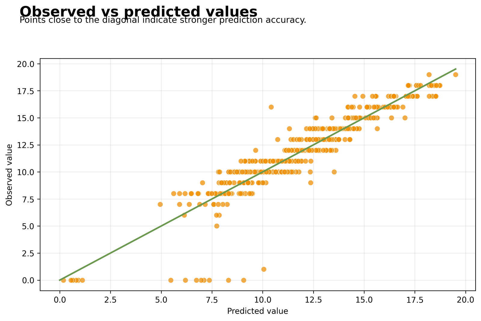
Most observations follow the diagonal agreement line, with the largest departures concentrated among very low observed outcomes.
The model achieves R² = 0.8522, RMSE = 1.2410, and MAE = 0.7799.
Earlier grades allow the equation to reproduce most middle and high outcomes closely. The largest overpredictions occur when students with plausible G1 and G2 values receive G3 = 0, suggesting that zero may reflect a process not fully captured by the predictors.
Prediction quality is strong for the main grade range, but the model should not be assumed equally reliable for zero outcomes. Those cases warrant substantive review and influence diagnostics.
Chart 3: Residuals Versus Predicted Values
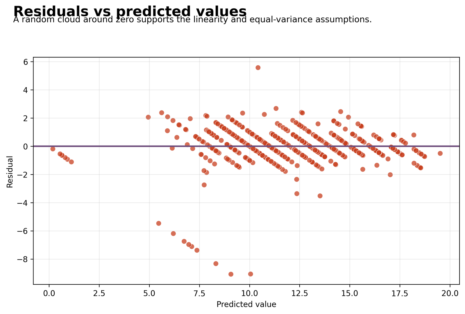
Residuals are concentrated around zero through most fitted values, with several large negative errors and visible diagonal bands.
Residual sum of squares is 999.4600, residual mean square is 1.5641, and residual degrees of freedom are 639.
The diagonal bands occur because observed grades are integers while predictions are continuous. The large negative residuals represent cases whose observed G3 is far below the value expected from their predictors. A mild shape in the cloud matters less than whether spread or curvature changes systematically.
The plot supports the model across the central range but highlights unusual low outcomes. Use studentized residuals, leverage, and Cook’s distance before deciding whether any case is influential.
Chart 4: Residual Distribution
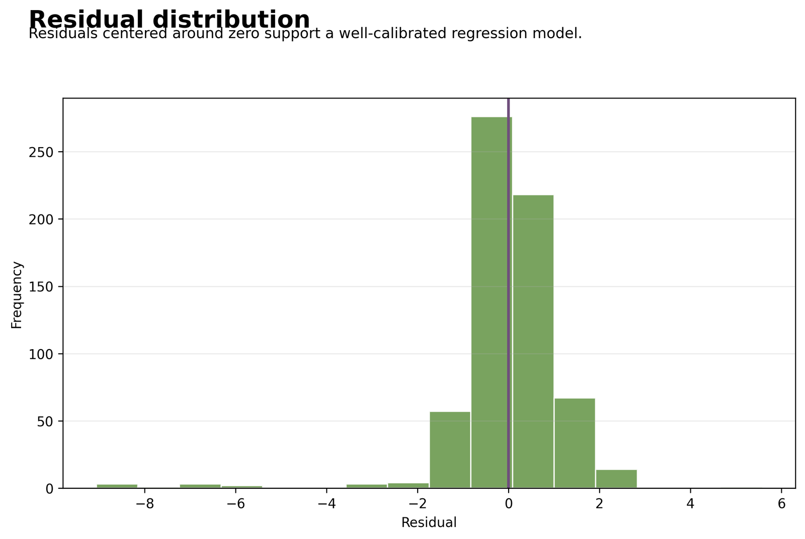
Most residuals cluster near zero, but the distribution has a long negative tail created by strong overprediction for a small number of observations.
The residual Shapiro–Wilk test has p < .001, while the sample size is 649.
The normality rejection does not mean the entire model is unusable. It indicates that the residual distribution departs from a perfect bell shape, mainly because of a limited set of unusually low outcomes. With this sample size, visual magnitude, robust sensitivity, and influence matter more than the test result alone.
Report the departure rather than hiding it. Confidence intervals and p-values should be checked for robustness, especially for coefficients close to the .05 threshold.
Chart 5: Residual Q–Q Plot
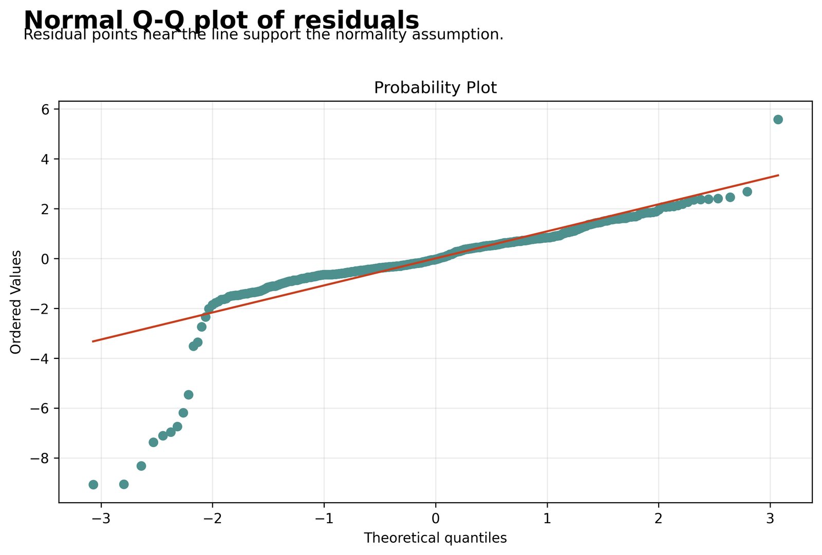
Points track the reference line through much of the centre and depart most strongly in the lower tail.
The accompanying Shapiro–Wilk result is p < .001; the centre of the Q–Q pattern is substantially closer to the line than the extreme lower tail.
Most ordinary prediction errors are approximately compatible with the normal reference, while a small group of negative residuals is more extreme than the distribution would predict. The problem is tail behaviour, not a complete failure of the central residual pattern.
Inference should acknowledge lower-tail non-normality. Robust standard errors or a sensitivity analysis excluding only well-justified special cases can show whether the main conclusions change.
Chart 6: Regression Coefficients
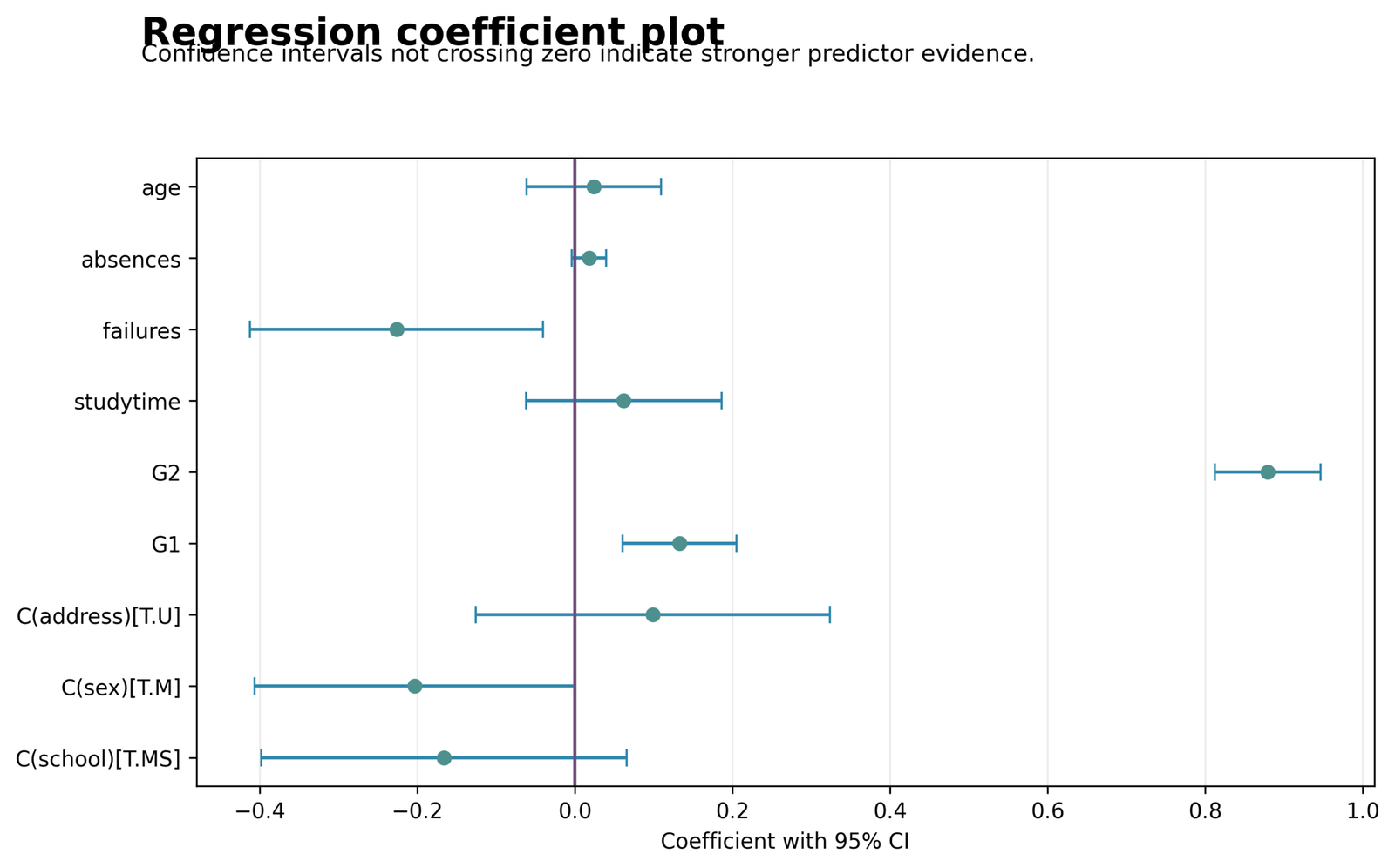
G2 has by far the largest positive coefficient. G1 remains positive, failures is negative, and the male coefficient is small and negative near the significance boundary.
G2: B = 0.8794, CI [0.8124, 0.9465]; G1: B = 0.1328, CI [0.0606, 0.2050]; failures: B = −0.2266, CI [−0.4127, −0.0406]; male: B = −0.2037, CI [−0.4068, −0.0007].
Second-period grade carries most of the unique predictive information. G1 contributes a smaller independent association, while each additional prior failure is linked to a modest reduction in expected G3. Several background variables add little once academic history is included.
Interpret effect size and uncertainty together. G2 is both precise and substantively large; the sex coefficient is much smaller and lies very close to zero, so it should not receive equal emphasis.
Chart 7: Model Fit Summary
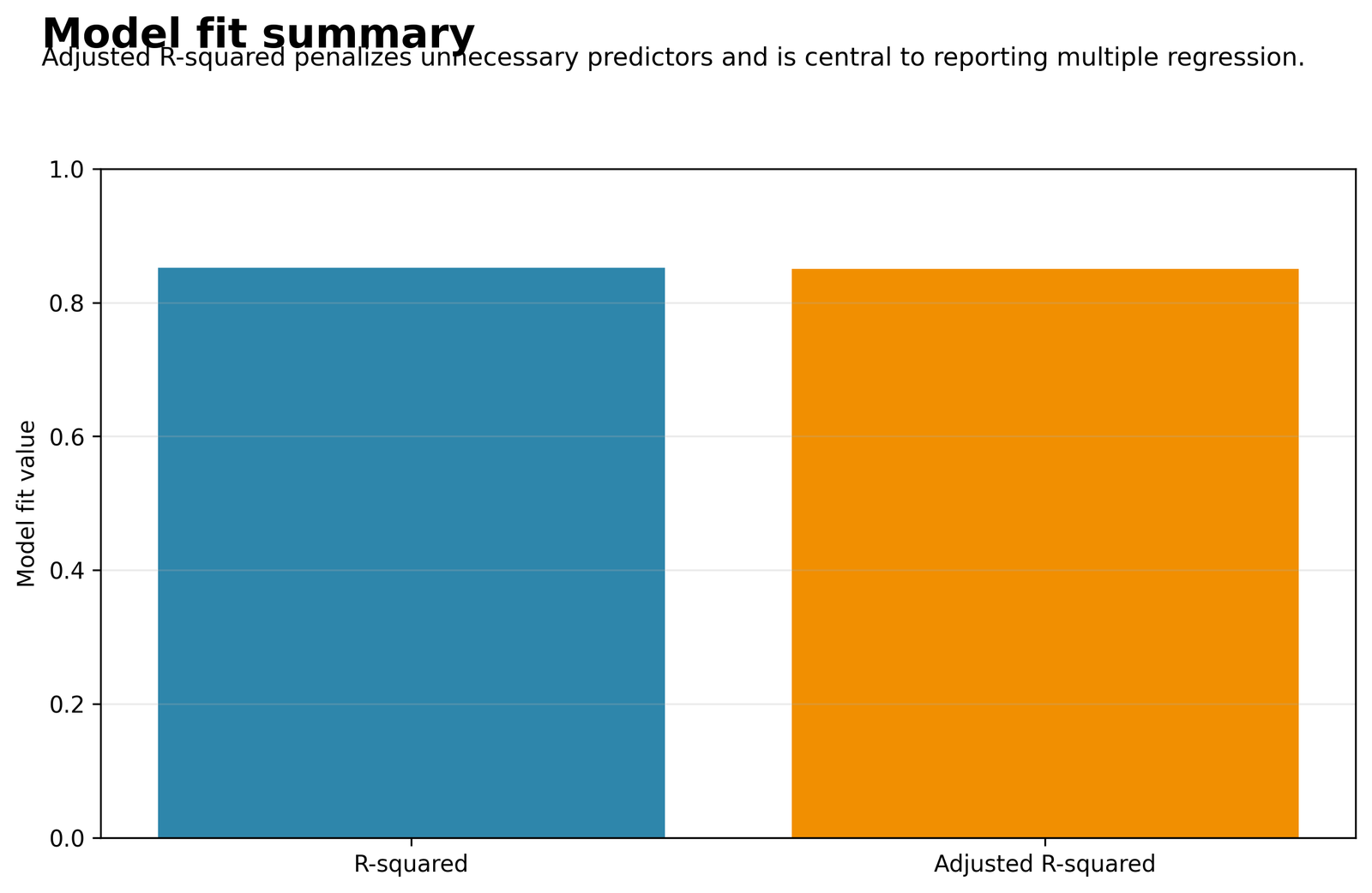
The model explains a large share of G3 variation, and adjusted R² remains almost identical to R².
R² = 0.8522, adjusted R² = 0.8501, F(9,639) = 409.4514, RMSE = 1.2410, and MAE = 0.7799.
The predictors collectively capture most of the systematic differences in final grades. The small gap between R² and adjusted R² indicates that the model is not gaining fit merely by adding unnecessary terms. Typical absolute prediction error is below one grade point, although larger errors remain for special cases.
Use fit statistics for different purposes: adjusted R² for explained variation, RMSE and MAE for prediction error, and the F test for evidence that the full predictor set improves on an intercept-only model.
Chart 8: Observed and Predicted G3 by G2

Observed and predicted G3 rise together across G2, with close agreement through the main data range.
The adjusted G2 slope is 0.8794. A one-point increase in G2 corresponds to about 0.88 additional expected G3 points, holding the other predictors constant.
G2 is the main bridge from earlier performance to final outcome. The fitted pattern follows the observed averages because students generally maintain similar performance between the second and final periods. Remaining vertical spread reflects the contribution of G1, failures, attendance, background variables, and individual error.
G2 provides the strongest basis for prediction and early support decisions. Students whose observed G3 falls far below the fitted trajectory are the cases most likely to require individual investigation.
R Chart Interpretations
The paired R figures use the same reader-facing interpretation structure and focus on the statistical pattern rather than software-specific repetition.
R Outcome Distribution
The central mass represents ordinary grade progression, while the zero outcomes create a long lower tail. Those zero cases are likely to produce the largest negative residuals because their G1 and G2 profiles may otherwise resemble students with nonzero final grades.
R Observed Versus Predicted G3
Earlier grades allow the equation to reproduce most middle and high outcomes closely. The largest overpredictions occur when students with plausible G1 and G2 values receive G3 = 0, suggesting that zero may reflect a process not fully captured by the predictors.
R Residuals Versus Predicted Values
The diagonal bands occur because observed grades are integers while predictions are continuous. The large negative residuals represent cases whose observed G3 is far below the value expected from their predictors. A mild shape in the cloud matters less than whether spread or curvature changes systematically.
R Residual Distribution
The normality rejection does not mean the entire model is unusable. It indicates that the residual distribution departs from a perfect bell shape, mainly because of a limited set of unusually low outcomes. With this sample size, visual magnitude, robust sensitivity, and influence matter more than the test result alone.
R Residual Q–Q Plot
Most ordinary prediction errors are approximately compatible with the normal reference, while a small group of negative residuals is more extreme than the distribution would predict. The problem is tail behaviour, not a complete failure of the central residual pattern.
R Regression Coefficients
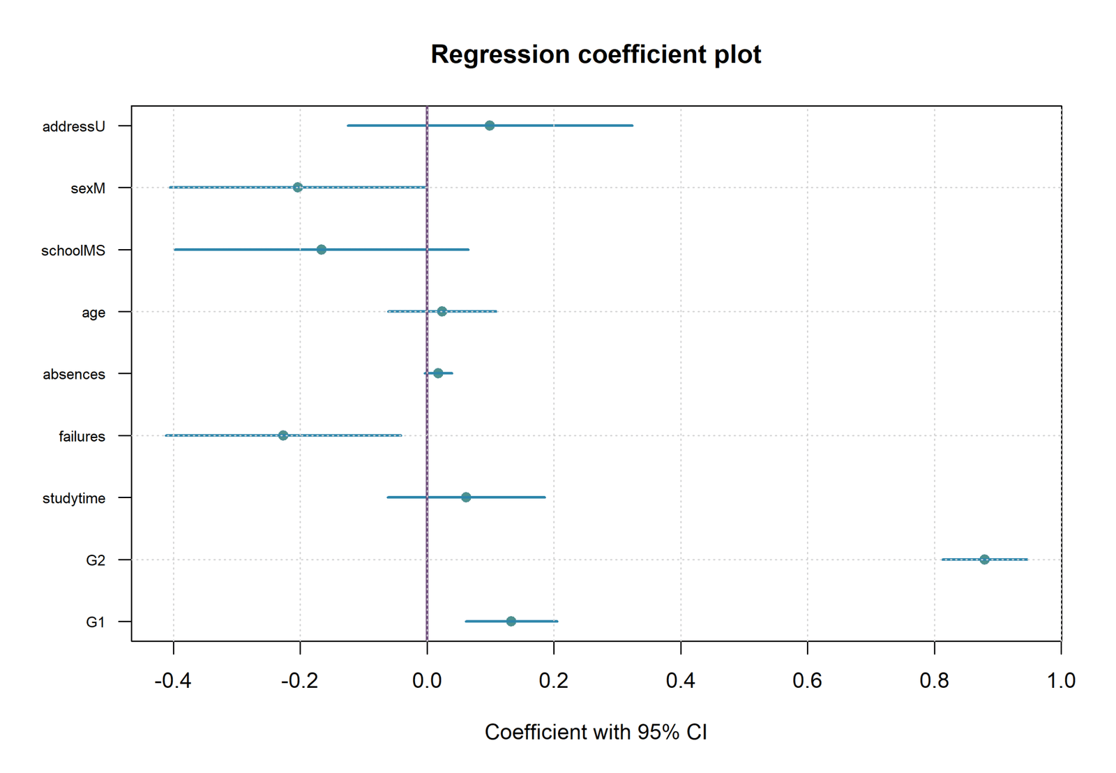
Second-period grade carries most of the unique predictive information. G1 contributes a smaller independent association, while each additional prior failure is linked to a modest reduction in expected G3. Several background variables add little once academic history is included.

R Model Fit Summary
The predictors collectively capture most of the systematic differences in final grades. The small gap between R² and adjusted R² indicates that the model is not gaining fit merely by adding unnecessary terms. Typical absolute prediction error is below one grade point, although larger errors remain for special cases.
R Observed and Predicted G3 by G2
G2 is the main bridge from earlier performance to final outcome. The fitted pattern follows the observed averages because students generally maintain similar performance between the second and final periods. Remaining vertical spread reflects the contribution of G1, failures, attendance, background variables, and individual error.
Ordinary Least Squares Regression Coefficients
| Term | B | SE | t | p | 95% CI | Meaning |
|---|---|---|---|---|---|---|
| Intercept | −0.2405 | 0.7779 | −0.3091 | .7573 | −1.7679 to 1.2870 | Not substantively meaningful at the all-zero setting |
| school MS | −0.1665 | 0.1181 | −1.4099 | .1590 | −0.3983 to 0.0654 | No reliable adjusted school difference |
| male | −0.2037 | 0.1034 | −1.9701 | .0493 | −0.4068 to −0.0007 | Small negative adjusted difference at the significance boundary |
| urban | 0.0989 | 0.1145 | 0.8636 | .3881 | −0.1260 to 0.3237 | No reliable adjusted address difference |
| G1 | 0.1328 | 0.0368 | 3.6121 | .0003 | 0.0606 to 0.2050 | Positive independent association |
| G2 | 0.8794 | 0.0342 | 25.7517 | <.001 | 0.8124 to 0.9465 | Dominant positive predictor |
| studytime | 0.0619 | 0.0632 | 0.9783 | .3283 | −0.0623 to 0.1860 | No reliable unique effect |
| failures | −0.2266 | 0.0947 | −2.3922 | .0170 | −0.4127 to −0.0406 | Additional failures predict lower G3 |
| absences | 0.0177 | 0.0112 | 1.5856 | .1133 | −0.0042 to 0.0396 | No reliable unique effect |
| age | 0.0236 | 0.0435 | 0.5432 | .5872 | −0.0618 to 0.1091 | No reliable unique effect |
The coefficient results should be read with P-Value and Confidence Interval. A coefficient can be statistically detectable but still small in practice, as illustrated by the male indicator. Conversely, G2 is large, precise, and central to both explanation and prediction.
Ordinary Least Squares Regression Predictions and Error Measures
RMSE
1.2410
Larger errors receive extra weight because residuals are squared before averaging.
MAE
0.7799
The average absolute difference between observed and predicted G3 is below one grade point.
Predictions represent conditional expected values, not guaranteed outcomes. A student may differ substantially from the fitted value because of omitted influences, measurement error, an unusual event, or a data process not represented by the equation.
The worked Excel file provides row-level predictions, residuals, squared residuals, absolute residuals, and a prediction calculator. Its expanded 15-predictor specification has R² = 0.8541 and adjusted R² = 0.8507, but those coefficients belong to that expanded model and should not be merged with the nine-predictor Python table.
Ordinary Least Squares Regression Assumptions and Diagnostics
Supported
- High model fit
- Residuals centred through the main range
- Acceptable VIF values
- No major R² inflation from extra terms
Requires attention
- Lower-tail residual non-normality
- Zero-outcome overprediction
- Potential influential cases
- Possible heteroskedasticity sensitivity
VIF values range from 1.0733 to 4.2214. G1 and G2 have the largest values, 4.2214 and 4.1019, but remain below common concern thresholds. Review Variance Inflation Factor and Tolerance Statistic alongside coefficient stability. This Ordinary Least Squares Regression result should be interpreted with the stated model specification and uncertainty.
The Shapiro–Wilk test rejects residual normality, but the Q–Q plot indicates that the largest departures are concentrated in the lower tail. Use Studentized Residuals, Cook’s Distance, and Influence Diagnostics to identify whether a small number of cases drive the departure.
Unequal variance should be assessed through the residual plot and formal checks such as the Breusch–Pagan Test or White Test. Functional form can be examined with residual curvature and the Ramsey RESET Test.
SPSS, Python, R and Excel Workflows
Python
Fits the nine-predictor OLS model, produces coefficient inference, VIF diagnostics, predictions, and eight figures. This Ordinary Least Squares Regression result should be interpreted with the stated model specification and uncertainty.
R
Uses lm(), summary(), anova(), and diagnostic plots for the same linear model structure.
SPSS
Uses the REGRESSION procedure for coefficients, confidence intervals, collinearity diagnostics, predicted values, and residuals.
Excel
The worked workbook contains an expanded 15-predictor model, coefficient table, row-level predictions, residual calculations, and a prediction calculator.
Code: Expand Only the Software You Need
Python Ordinary Least Squares Regression code
import pandas as pd
import statsmodels.formula.api as smf


df = pd.read_csv("dataset.csv")
formula = (
    "G3 ~ G1 + G2 + studytime + failures + absences + age + "
    "C(school) + C(sex) + C(address)"
)
model = smf.ols(formula, data=df).fit()
print(model.summary())
df["predicted_G3"] = model.predict(df)
df["residual"] = df["G3"] - df["predicted_G3"]
R Ordinary Least Squares Regression code
df <- read.csv("dataset.csv")
fit <- lm(
  G3 ~ G1 + G2 + studytime + failures + absences + age +
    school + sex + address,
  data = df
)
summary(fit)
anova(fit)
par(mfrow = c(2, 2))
plot(fit)
SPSS Ordinary Least Squares Regression syntax
REGRESSION
 /DEPENDENT G3
 /METHOD=ENTER G1 G2 studytime failures absences age school_MS sex_M address_U
 /STATISTICS COEFF OUTS R ANOVA CI(95) COLLIN
 /SAVE PRED RESID SRESID COOK LEVER.
Excel prediction equation
Predicted G3 = Intercept
 + B_G1*G1 + B_G2*G2 + B_studytime*studytime
 + B_failures*failures + B_absences*absences
 + B_age*age + B_school*school_dummy
 + B_sex*sex_dummy + B_address*address_dummy

Residual = Observed G3 - Predicted G3
Squared residual = Residual^2
Absolute residual = ABS(Residual)
Advanced Ordinary Least Squares Regression Interpretation
R-squared and adjusted R-squared
R² measures the proportion of observed outcome variation represented by the fitted values. Adjusted R² penalizes unnecessary predictors and is preferred when comparing models with different numbers of terms. See Adjusted R-Squared. This Ordinary Least Squares Regression result should be interpreted with the stated model specification and uncertainty.
The model F test
For Ordinary Least Squares Regression, The F test compares the fitted model with an intercept-only model. A significant result indicates that the predictor set improves prediction collectively; it does not show that every individual coefficient is significant.
Partial regression coefficients
Within an Ordinary Least Squares Regression model, Each slope estimates a conditional association. The coefficient for G1 is not its raw association with G3; it is the remaining relationship after G2 and the other predictors are controlled.
Categorical predictors
When interpreting Ordinary Least Squares Regression, Indicator coefficients compare each coded category with a reference category while all remaining predictors are held constant. The reference group must be stated for meaningful interpretation.
Prediction intervals
In Ordinary Least Squares Regression, A confidence interval estimates uncertainty around the mean expected outcome. A prediction interval is wider because it also includes person-level residual variation.
RMSE versus MAE
For Ordinary Least Squares Regression, RMSE penalizes large errors more strongly; MAE describes the average absolute error in the original outcome unit. Reporting both distinguishes general accuracy from sensitivity to extreme errors.
Residual normality
Within an Ordinary Least Squares Regression model, Normality applies to residuals, not necessarily to the raw outcome or predictors. Large samples can produce significant normality tests for modest tail departures.
Homoscedasticity
When interpreting Ordinary Least Squares Regression, Homoscedasticity means residual variance is reasonably stable across fitted values. Unequal spread can distort conventional standard errors even when coefficients remain unbiased under exogeneity.
Linearity
In Ordinary Least Squares Regression, Linearity concerns the conditional mean. Curvature in residual plots suggests polynomial, spline, transformation, or nonlinear modelling may be more appropriate.
Independence
For Ordinary Least Squares Regression, OLS assumes errors are independent under the ordinary model. Repeated observations, classrooms, families, clinics, or geographic units may require clustered, mixed, fixed-effects, or GEE methods.
Multicollinearity
Within an Ordinary Least Squares Regression model, High predictor overlap inflates coefficient standard errors and can make individual effects unstable. Prediction may remain strong even when coefficient interpretation becomes difficult.
Influential cases
When interpreting Ordinary Least Squares Regression, Influence combines residual size and leverage. A case should not be removed simply because it is influential; its validity and substantive meaning must be investigated first.
Omitted-variable bias
In Ordinary Least Squares Regression, A coefficient has a causal interpretation only under strong design and no-unmeasured-confounding assumptions. Good prediction does not by itself establish causation.
Standardized coefficients
For Ordinary Least Squares Regression, Standardization expresses numeric effects in standard-deviation units. It can aid comparison but does not replace the original-unit coefficients needed for practical interpretation.
Interaction terms
Within an Ordinary Least Squares Regression model, An interaction allows one predictor slope to change across another variable. Lower-order terms must remain in the model, and interpretation should use conditional slopes or predictions.
Polynomial terms
When interpreting Ordinary Least Squares Regression, Polynomial regression remains linear in coefficients even when predictors are squared or cubed. It is useful for smooth curvature but can behave poorly outside the observed range.
Robust standard errors
In Ordinary Least Squares Regression, Heteroskedasticity-consistent standard errors can test whether conclusions survive unequal variance. They modify inference, not the fitted coefficients.
Cross-validation
For Ordinary Least Squares Regression, In-sample R² can overstate performance on new data. Cross-validation or a held-out test set provides a stronger assessment of predictive generalization.
Model selection
Within an Ordinary Least Squares Regression model, Selection should combine theory, adjusted fit, prediction error, diagnostics, and interpretability rather than rely on automated p-value rules alone.
OLS versus generalized least squares
When interpreting Ordinary Least Squares Regression, Generalized Least Squares Regression is preferable when the error covariance structure is known or can be modelled credibly. OLS remains simpler and often sufficient when residual independence and stable variance are plausible.
OLS versus generalized additive models
In Ordinary Least Squares Regression, Generalized Additive Model can capture nonlinear predictor effects without specifying a fixed polynomial degree. OLS is preferable when the relationship is adequately linear and direct slopes are the reporting priority.
Statistical versus practical significance
For Ordinary Least Squares Regression, A small p-value does not guarantee a meaningful effect. Use coefficient units, confidence intervals, prediction improvement, and Effect Size to judge importance.
Reporting negative findings
Within an Ordinary Least Squares Regression model, Nonsignificant coefficients are informative when their confidence intervals exclude effects large enough to matter. They should not be described as proof of no relationship.
External validity
When interpreting Ordinary Least Squares Regression, The fitted equation reflects the sampled schools, students, measures, and time period. Performance should be reassessed before applying it to a different educational system or population.
Reproducible reporting
State the formula, coding, reference categories, sample size, missing-data handling, software, coefficient table, model fit, error metrics, and diagnostic findings.
Responsible prediction
Predictions should support—not replace—professional judgment. Cases near important decision thresholds deserve uncertainty intervals and contextual review.
APA-Style Ordinary Least Squares Regression Reporting
G2 was the strongest positive predictor, B = 0.879, SE = 0.034, t = 25.75, p < .001, 95% CI [0.812, 0.947]. G1 also remained positive, B = 0.133, p < .001, while failures was negative, B = −0.227, p = .017. Residual diagnostics indicated lower-tail non-normality, so influential cases and robust sensitivity should be reported. This Ordinary Least Squares Regression result should be interpreted with the stated model specification and uncertainty.
Publication Checklist and Common Mistakes
Include
- Outcome and predictor definitions
- Reference categories
- Model equation
- R² and adjusted R²
- F test
- Coefficients with 95% CIs
- RMSE and MAE
- Residual and influence diagnostics
Avoid
- Calling association causation
- Reporting R² without error metrics
- Ignoring residual structure
- Removing unusual cases automatically
- Mixing coefficients from different model specifications
- Repeating headings in the explanatory text
Connect inference to Null and Alternative Hypothesis, Type I and Type II Error, P-Value, Confidence Interval, and Statistical Power.
Downloads
Frequently Asked Questions
What is Ordinary Least Squares Regression?
When is OLS regression used?
What is the outcome here?
How many cases were analysed?
How much variation does the model explain?
What is the strongest predictor?
What does the G2 coefficient mean?
What do RMSE and MAE mean?
Is the overall model significant?
Are residuals normal?
Is multicollinearity severe?
Does a high R-squared prove causation?
Why do the Python and Excel coefficients differ?
Can categorical predictors be included?
What is the difference between OLS and correlation?
How should OLS be reported?
Final Ordinary Least Squares Regression Conclusion
The model provides a strong account of final-grade differences. G2 carries most of the unique predictive information, G1 adds a smaller independent association, and prior failures are linked to a modest reduction in expected G3. The remaining variables contribute little once academic history is controlled.
Fit is high and average prediction error is low, but the residual diagnostics identify a lower-tail group that the equation overpredicts. The strongest report therefore combines the high R-squared with the error metrics, coefficient uncertainty, and an honest discussion of unusual low outcomes.

