
Partial Least Squares Regression: Tutorial, Interpretation, Python, R, SPSS and Excel Guide
Partial Least Squares Regression builds outcome-focused latent components from correlated predictors and uses those components to estimate a continuous response. This worked example predicts G3 from twelve design variables and selects five components through cross-validation.
12 design predictors
5 selected components
R² = 0.8515
Model Overview
Partial Least Squares Regression, commonly shortened to PLS regression, is a supervised dimension-reduction method for predicting one or more outcomes from a set of predictors that may be numerous, highly correlated, noisy, or difficult to interpret separately. The method replaces the original predictors with a smaller collection of latent components and then uses those components in the prediction model.
The term partial least square regression is also used in search and software documentation, although Partial Least Squares Regression is the standard name. “Partial least squares” refers to the algorithm’s construction of latent scores from the predictor matrix and outcome information. “Regression” refers to the final relationship between those scores and the response.
What is Partial Least Squares Regression designed to answer? It estimates how well a smaller set of supervised latent dimensions can predict an outcome and identifies which original variables contribute most to those dimensions. It is particularly useful when ordinary Multiple Linear Regression is unstable because predictors overlap strongly, when the number of predictors is large relative to the sample, or when prediction is more important than classical coefficient-by-coefficient inference.
Partial Least Squares Regression works by searching for weighted combinations of the predictors that have high covariance with the outcome. Each component is constructed to retain information from X while remaining directly relevant to Y. Later components explain additional predictive structure after the earlier component information has been extracted.
This supervised construction separates Partial Least Squares Regression from principal component analysis and principal component regression. Principal components regression first finds directions that explain predictor variance without using the outcome, then regresses Y on selected principal components. PLS regression allows Y to guide component construction from the beginning. A predictor direction with modest X variance can therefore be retained when it has strong outcome relevance.
The distinction between principal components regression and Partial Least Squares Regression is one of the most common search questions. Neither method is universally superior. Principal components regression can be useful when representing X is the main goal, whereas PLS regression is usually more directly aligned with prediction because the response contributes to the latent directions.
Partial Least Squares Regression also differs from ordinary least squares and multiple linear regression. OLS estimates coefficients directly in the original predictor space and is attractive when the sample is adequate, multicollinearity is manageable, and inferential interpretation is central. PLS reduces the predictor space before reconstructing a prediction equation. This often improves stability under collinearity, but the reconstructed coefficients do not automatically carry standard OLS p-values or confidence intervals.
When to use Partial Least Squares Regression depends on the data and research goal. Common situations include spectroscopy, chemometrics, metabolomics, neuroscience, marketing research, sensor data, image-derived features, and other applications with many correlated measures. It is also useful in smaller educational or clinical examples when researchers want to demonstrate supervised component selection, coefficient reconstruction, variable importance in projection, and cross-validated prediction.
The method supports continuous numeric predictors and can incorporate categorical variables after appropriate dummy coding. Because the latent components depend on scale, numeric predictors are commonly standardized. The number of components is a tuning parameter and should be selected through cross-validation rather than by maximizing training fit.
Partial Least Squares Regression assumptions are less focused on predictor independence than ordinary least squares assumptions. Correlated predictors are expected rather than prohibited. The analysis still requires a meaningful outcome, a reasonably linear predictive relationship in the transformed space, representative observations, careful treatment of missing values, protection against extreme outliers, and validation that reflects the intended population. Independence remains important when ordinary cross-validation is used; grouped or time-aware validation may be needed for clustered or longitudinal data.
Coefficients, component scores, loadings, cross-validation error, and VIP scores answer different questions. Coefficients reconstruct the prediction equation in the original design columns. Scores locate observations in the latent component space. Loadings describe how variables relate to components. VIP scores summarize a variable’s contribution across the selected components. None of these should be treated as a substitute for external validation.
In this Partial Least Squares Regression example, G3 is the outcome. Numeric predictors are G1, G2, studytime, failures, absences, age, Medu, and Fedu. School, sex, address, and famsize are dummy coded, producing twelve design columns. Five components are selected from models containing one through five components.
The final Partial Least Squares Regression model explains 85.15% of G3 variation and has RMSE = 1.2442 and MAE = 0.7843. G2 has the largest reconstructed coefficient and the highest VIP score, while G1 is the only other predictor above the conventional VIP threshold of 1.
Quick Answer
Prediction results
- Adjusted R²: 0.8503
- RMSE: 1.2442
- MAE: 0.7843
- SSE: 1004.6828
Predictor ranking
- G2 VIP: 2.1711
- G1 VIP: 1.9192
- Failures VIP: 0.9546
- Best tested CV RMSE: 0.3905
Table of Contents
- What is Partial Least Squares Regression?
- When to use Partial Least Squares Regression
- How Partial Least Squares Regression works
- PLS vs principal component and multiple linear regression
- Partial Least Squares Regression assumptions
- Variables and design matrix
- Results at a glance
- Eight Python chart explanations
- Partial Least Squares Regression in R
- Coefficients and VIP scores
- Prediction equation and component selection
- Diagnostics and validation
- Python, R, SPSS and Excel
- Code and software steps
- Advanced Partial Least Squares Regression topics
- APA-style reporting
- Publication checklist
- Downloads
- Related Salar Cafe guides
- Frequently asked questions
What Partial Least Squares Regression Is and When It Is Used
What Is Partial Least Squares Regression?
Partial Least Squares Regression is a prediction method that compresses correlated predictors into latent components chosen with direct reference to the outcome. The components are weighted sums of the original design columns and are extracted sequentially.
A simple explanation of Partial Least Squares Regression is that it searches for a small number of hidden predictor patterns that matter for Y. Instead of asking twelve correlated predictors to compete separately in one unstable equation, the method combines their shared information into supervised dimensions.
The method is often described as projection on latent structures. That name emphasizes that observations are projected into a lower-dimensional score space before the outcome is estimated. The final coefficients then translate the component model back into the original predictor columns.
This structure makes Partial Least Squares Regression both a dimension-reduction method and a regression model. It is not the same as partial correlation, Partial Correlation, ordinary least squares, or a structural equation model using the similar abbreviation PLS-SEM.
When to Use Partial Least Squares Regression
Partial Least Squares Regression is used when predictor collinearity makes ordinary coefficient estimates unstable, when the design matrix is wide, or when an outcome-focused reduction is preferable to an unsupervised reduction.
It can also be selected when researchers need one model to combine dimension reduction, prediction, component selection, and variable ranking. Chemometrics and spectroscopy are classic applications, but Partial Least Squares Regression appears in biological data, imaging, ecology, marketing, engineering, and machine learning workflows.
The method is less attractive when the principal goal is a causal coefficient with a conventional standard error and p-value for each predictor. In that setting, a well-specified Multiple Linear Regression model, Generalized Linear Model, penalized regression, or design-based estimator may answer the question more directly.
How Partial Least Squares Regression Works, Compares, and Is Validated
Encode categories, handle missing values, and standardize predictors.
Find predictor scores with high covariance with the outcome.
Choose the number of components through cross-validation.
Transform the component solution into fitted outcomes and predictor coefficients.
The score vector tₕ is a weighted combination of predictor columns. Each component captures outcome-relevant structure not already represented by earlier components. After component extraction, the model reconstructs a coefficient matrix B for prediction in the original design space.
Scaling is important because variables measured on larger numeric ranges could otherwise dominate the component weights. Dummy variables also enter the scaled design and should be interpreted with their reference categories in mind.
Partial Least Squares vs Principal Component and Multiple Linear Regression
| Method | How dimensions are chosen | Strength | Main caution |
|---|---|---|---|
| Partial Least Squares Regression | Uses covariance between predictors and outcome | Outcome-focused reduction under collinearity | Component and coefficient interpretation requires care |
| Principal component regression | Uses predictor variance without the outcome | Stable unsupervised representation of X | High-variance components may not be predictive |
| Multiple linear regression | No dimension reduction | Direct coefficient interpretation and standard inference | Can be unstable with severe multicollinearity or high dimensionality |
| Elastic Net Regression | Penalizes original coefficients | Prediction and variable selection with correlated predictors | Penalty tuning changes coefficient shrinkage |
The high-volume question “principal components regression partial least squares” is best answered through the role of Y. Principal component regression ignores Y while constructing components; Partial Least Squares Regression uses Y during component extraction.
For Partial Least Squares vs multiple linear regression, the choice depends on the intended result. Multiple linear regression is usually easier to report when individual effects and confidence intervals are the main goal. Partial Least Squares Regression is often stronger when prediction must remain stable despite correlated or numerous predictors.
Elastic Net Regression and Lasso Regression retain the original variable space while shrinking coefficients. PLS retains all predictors indirectly through a smaller latent space. These approaches can be compared through nested cross-validation rather than training R².
Partial Least Squares Regression Assumptions and Data Requirements
Required decisions
- A meaningful continuous response
- Consistent coding of numeric and categorical predictors
- Scaling appropriate to variable units
- A validation strategy matched to the data structure
- A component range selected before examining the test set
Diagnostic concerns
- Nonlinear relationships
- Influential observations
- Data leakage during scaling or selection
- Unstable components across resamples
- Dependent observations handled with ordinary random folds
Partial Least Squares Regression does not require predictors to be independent. Correlation among predictors is one of the reasons to use the method. It also does not rely on residual normality in the same way as a classical OLS significance test when the goal is prediction.
Linearity remains important because standard PLS regression builds linear latent scores and a linear response model. Nonlinear effects may require transformed variables, interaction terms, kernel PLS, or Generalized Additive Model methods.
Outliers can rotate component directions and affect both coefficients and VIP rankings. Use Outlier Detection, Cook’s Distance, and validation sensitivity analyses rather than assuming latent modelling automatically protects against unusual observations.
Variables and Design Matrix
| Variable | Role | Definition | Design treatment |
|---|---|---|---|
| G3 | Outcome | Final grade | Continuous response |
| G1 | Numeric predictor | First-period grade | Scaled numeric column |
| G2 | Numeric predictor | Second-period grade | Scaled numeric column |
| studytime | Numeric predictor | Study-time category | Scaled numeric column |
| failures | Numeric predictor | Prior failures | Scaled numeric column |
| absences | Numeric predictor | School absences | Scaled numeric column |
| age | Numeric predictor | Age in years | Scaled numeric column |
| Medu, Fedu | Numeric predictors | Maternal and paternal education | Scaled numeric columns |
| school | Categorical predictor | GP or MS | school_MS dummy |
| sex | Categorical predictor | F or M | sex_M dummy |
| address | Categorical predictor | R or U | address_U dummy |
| famsize | Categorical predictor | GT3 or LE3 | famsize_LE3 dummy |
The final design matrix contains twelve columns. Partial Least Squares Regression with categorical variables is therefore possible after reference-coded dummy variables are created and processed consistently inside each validation fold.
Partial Least Squares Regression Results at a Glance
Lowest tested CV RMSE
Strong in-sample fit
Adjusted using 5 components
Original G3 scale
Typical absolute error
Scaled outcome
Eight Partial Least Squares Regression Chart Explanations
Each figure is organized around the visible pattern, the values that define it, the statistical interpretation, and its relevance to prediction.
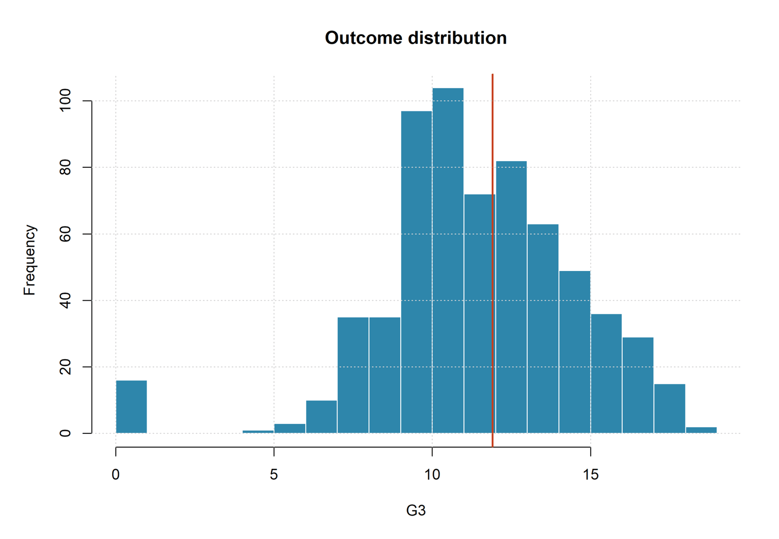
Chart 1: G3 Outcome Distribution
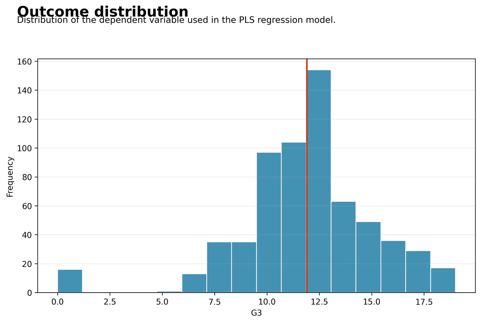
Most G3 values fall between about 9 and 15, with the highest frequency near 12. A separate group of zero scores creates a long lower tail.
The analysis contains 649 students. G3 has mean 11.906, standard deviation approximately 3.231, and observed range 0–19.
The central distribution is compact enough for stable prediction, but the zero-grade cases differ substantially from the majority. Their predictor profiles often resemble students with nonzero final grades, which makes them harder for a continuous prediction model to reproduce.
The outcome structure explains why the model performs well across the main grade range but produces some large negative residuals for zero outcomes. Background concepts are covered in Descriptive Statistics, Histogram Interpretation, and Standard Deviation.
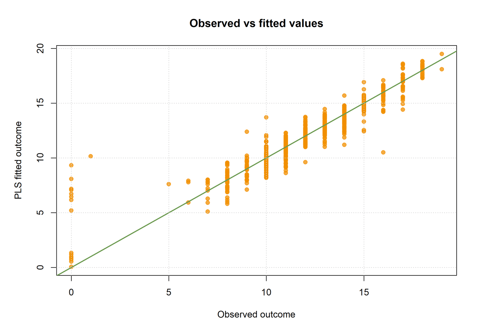
Chart 2: Observed Versus Fitted G3
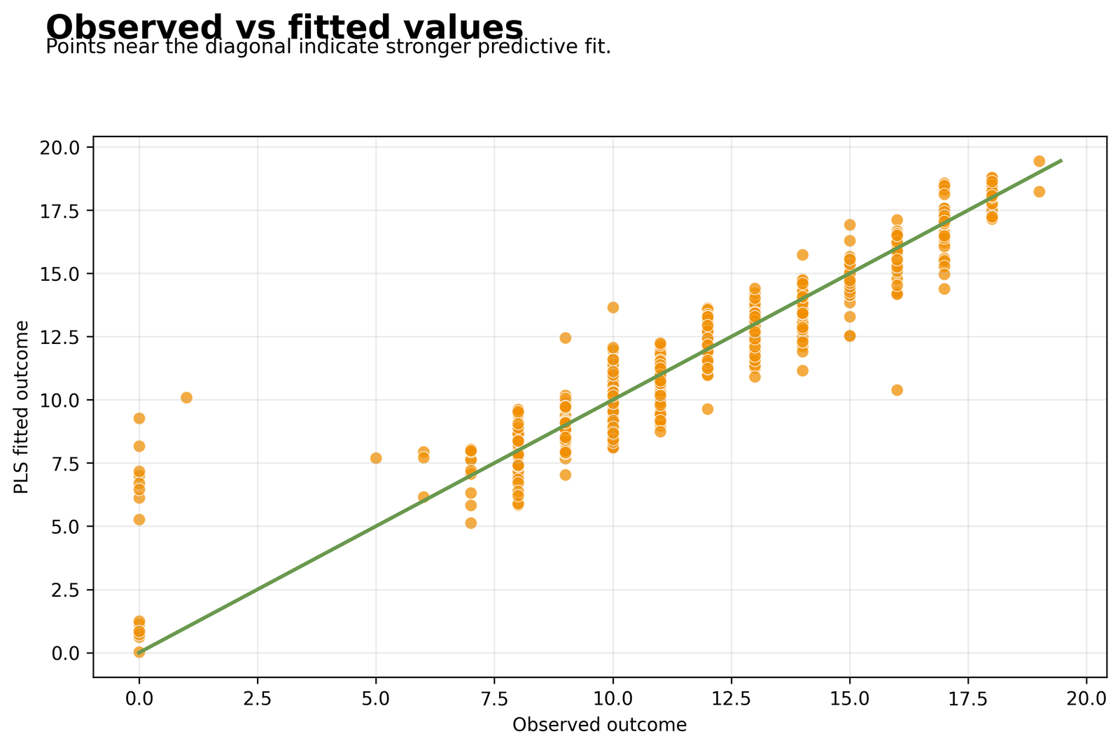
Predictions track the diagonal closely from the middle to the upper grade range. Observations with G3 = 0 spread vertically from fitted values near 0 to about 10.
R² = 0.8515, adjusted R² = 0.8503, RMSE = 1.2442, and MAE = 0.7843. The model uses 5 latent components built from 12 design predictors.
The latent components retain nearly all of the predictive information needed to estimate ordinary grade outcomes. The largest misses occur among students with zero final grades because the model combines their otherwise typical predictor values into midrange predictions.
The model is strong for prediction across the main data range, but its performance is not uniform. Decisions involving unusually low outcomes should consider the residual pattern rather than relying on the overall R² alone.
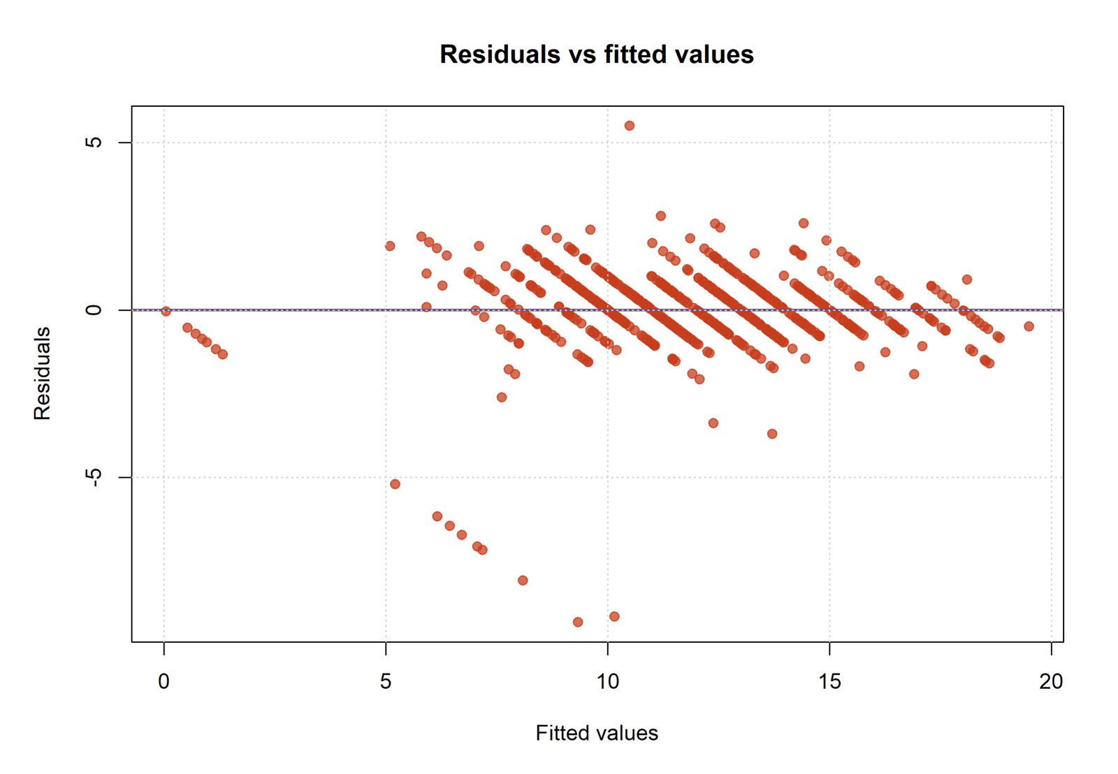
Chart 3: Residuals Versus Fitted Values
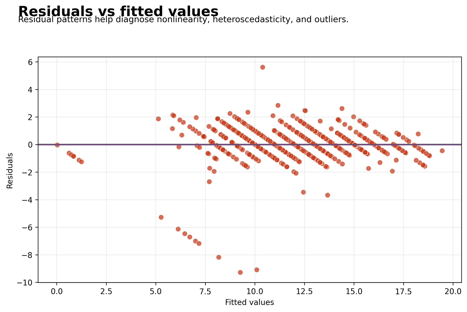
Most residuals lie between approximately −2 and +2. Diagonal bands run downward because G3 is recorded as integer grades. Several residuals fall below −6, and one positive residual is above +5.
The fitted model has RMSE = 1.2442 and MAE = 0.7843. The most extreme negative residuals occur around fitted grades of roughly 6–10.
Prediction error is small for most students, but the model substantially overpredicts a limited set of zero-grade cases. The diagonal bands are a consequence of the discrete outcome scale, not evidence that the fitted relationship repeatedly reverses.
Residual diagnostics identify where the prediction equation is least reliable. Review Studentized Residuals, Cook’s Distance, and Influence Diagnostics before treating unusual cases as data errors.
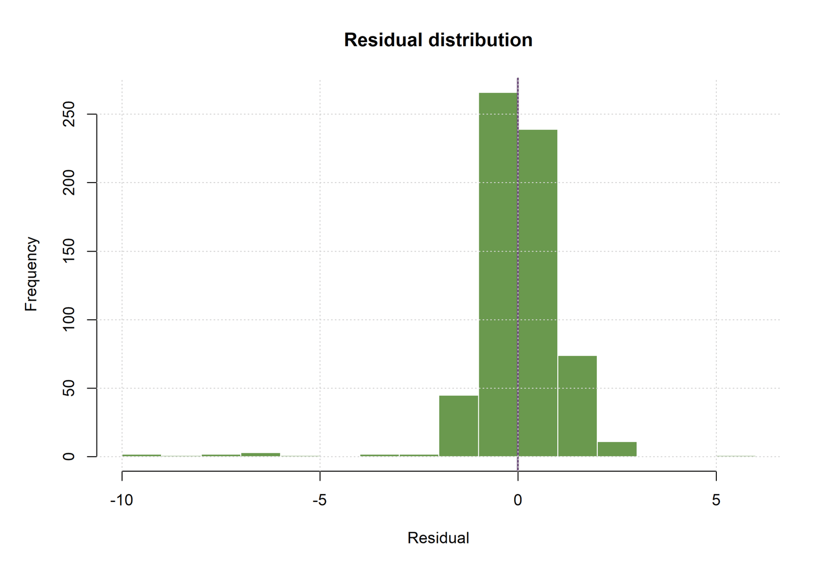
Chart 4: Residual Distribution
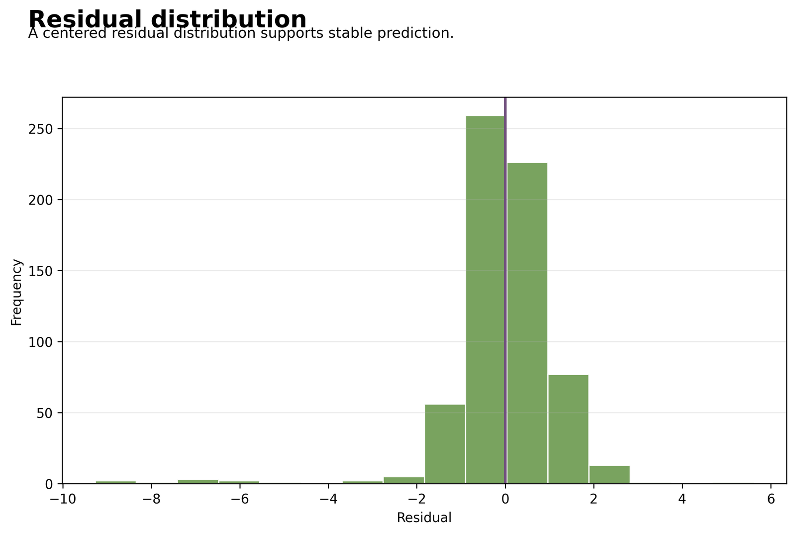
The highest bars fall around residuals from −1 to +1. The positive tail ends near +3 for most cases, while a thin negative tail extends toward −9.
The mean residual is close to 0 by construction. Most errors are small enough to support MAE = 0.7843, but the zero-grade cases increase RMSE to 1.2442 because squared error gives large misses more weight.
Typical prediction error is modest, yet the error distribution is not symmetric. A small number of severe overpredictions have a greater effect on RMSE than on MAE, which explains the gap between the two metrics.
Reporting both RMSE and MAE gives a more complete performance summary. Normality is not the primary goal of Partial Least Squares Regression prediction, but Q-Q Plot Normality Check can help describe the error distribution when inferential extensions are considered.
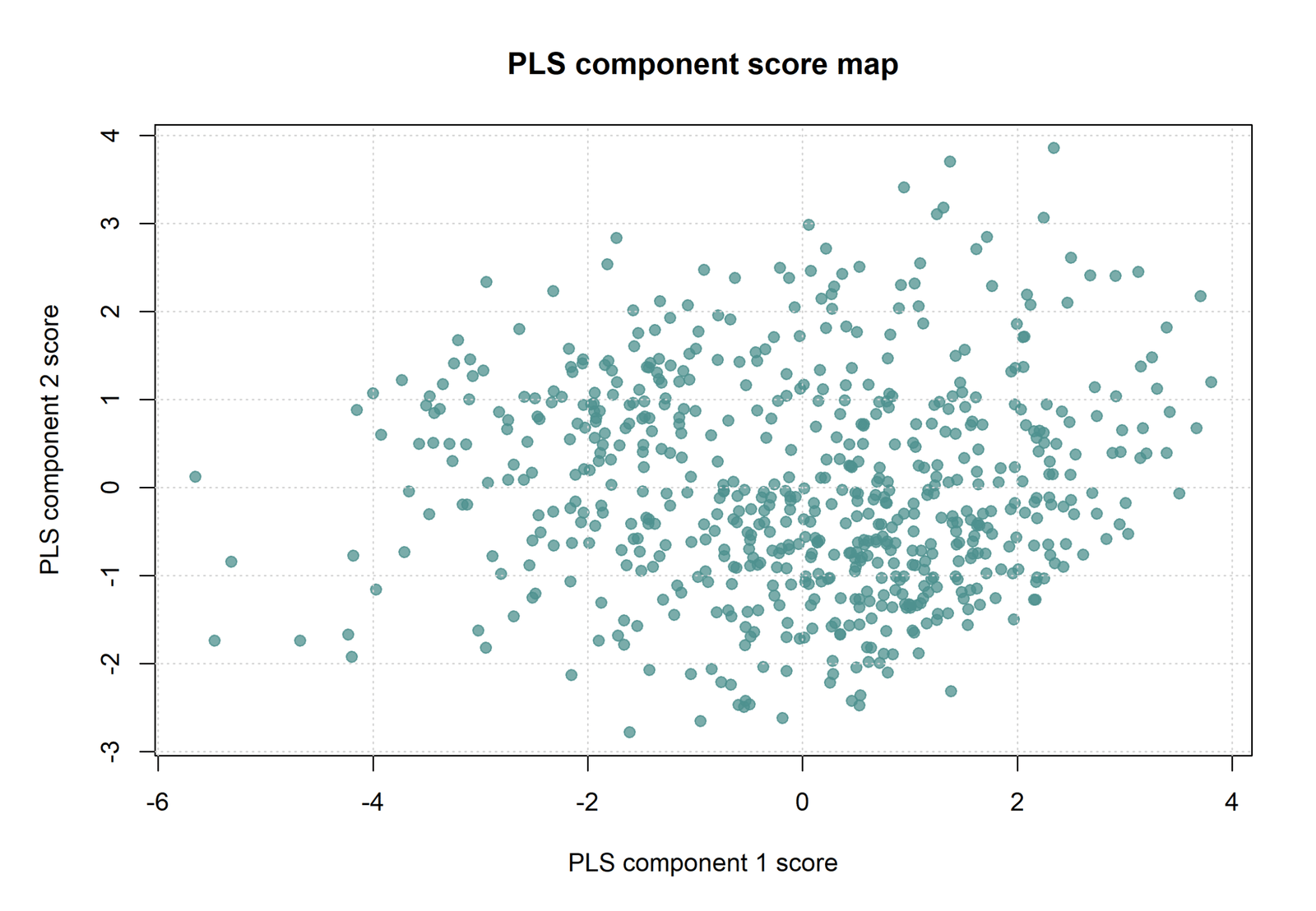
Chart 5: PLS Component Score Map
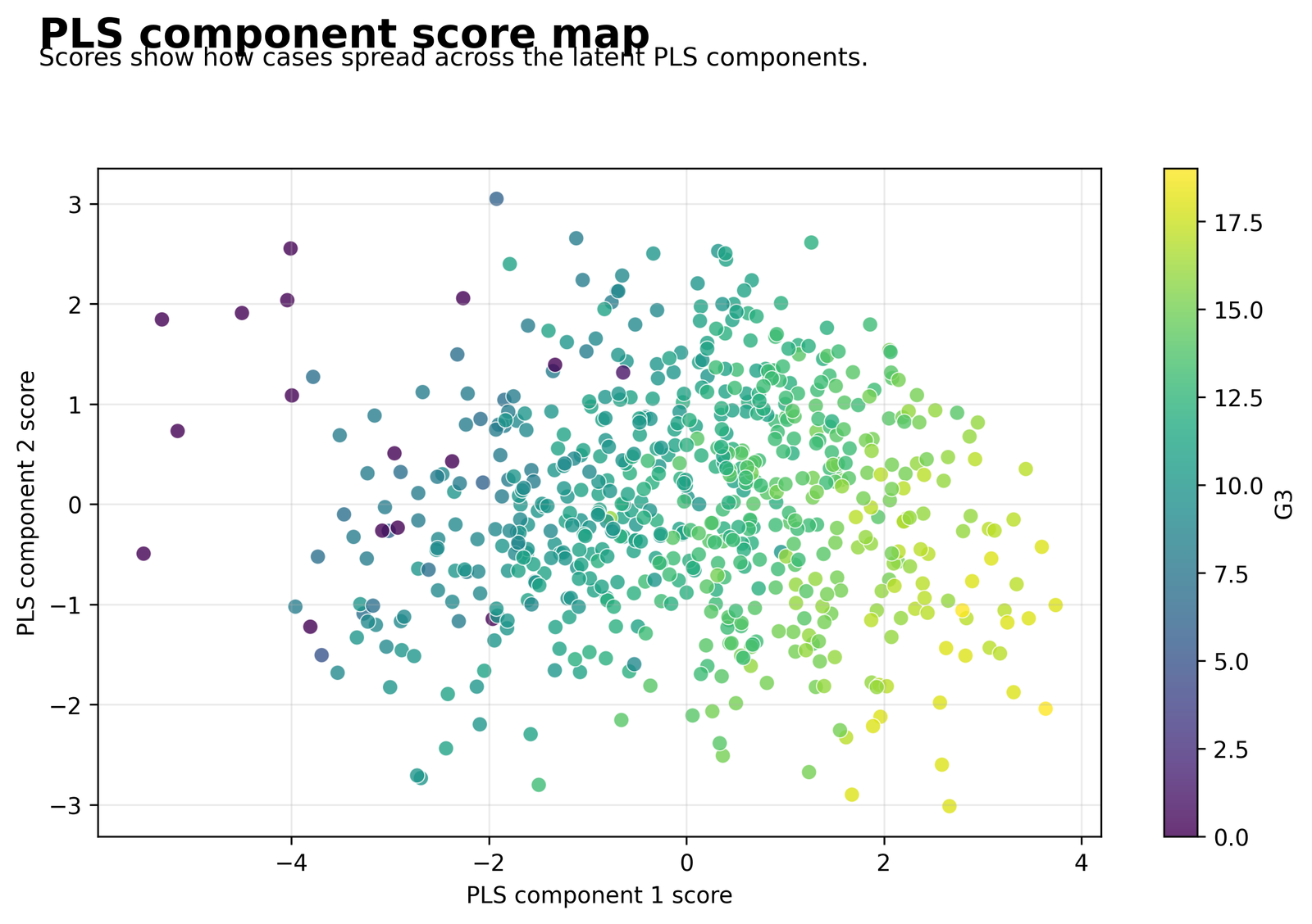
Lower G3 values are concentrated toward the left side of component 1, while higher G3 values become more common toward the right. Component 2 adds vertical spread but less obvious outcome ordering.
Component 1 scores extend approximately from −5 to +4, and component 2 scores from about −3 to +3. The color scale covers G3 values from 0 to 19.
The first latent component captures a combination of predictors that aligns strongly with final grade. Component 2 represents additional predictor structure that improves prediction without separating the outcome as strongly on its own. Overlap remains because students with similar latent scores can still have different final outcomes.
Component scores reduce twelve correlated design columns to a smaller supervised coordinate system. They are useful for understanding structure, but they are not original variables and should not be interpreted as direct measurements such as grade or studytime.
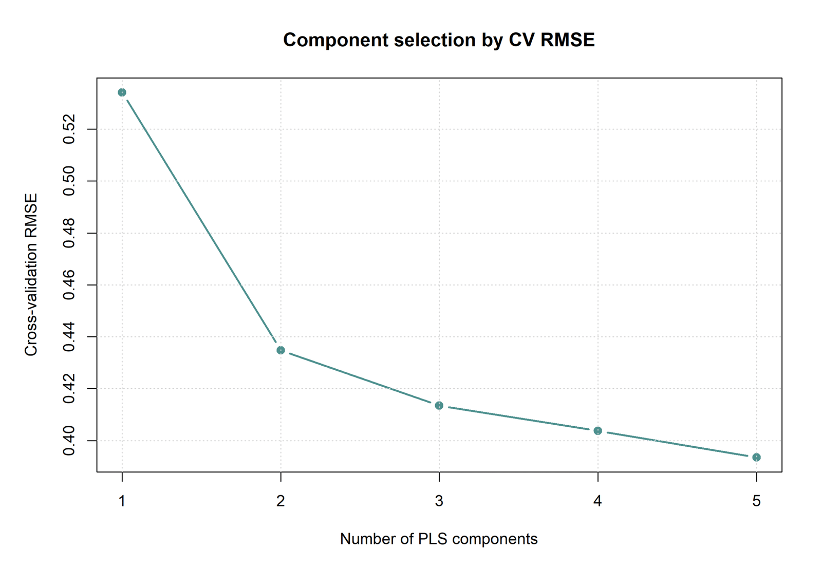
Chart 6: Cross-Validation RMSE by Number of Components
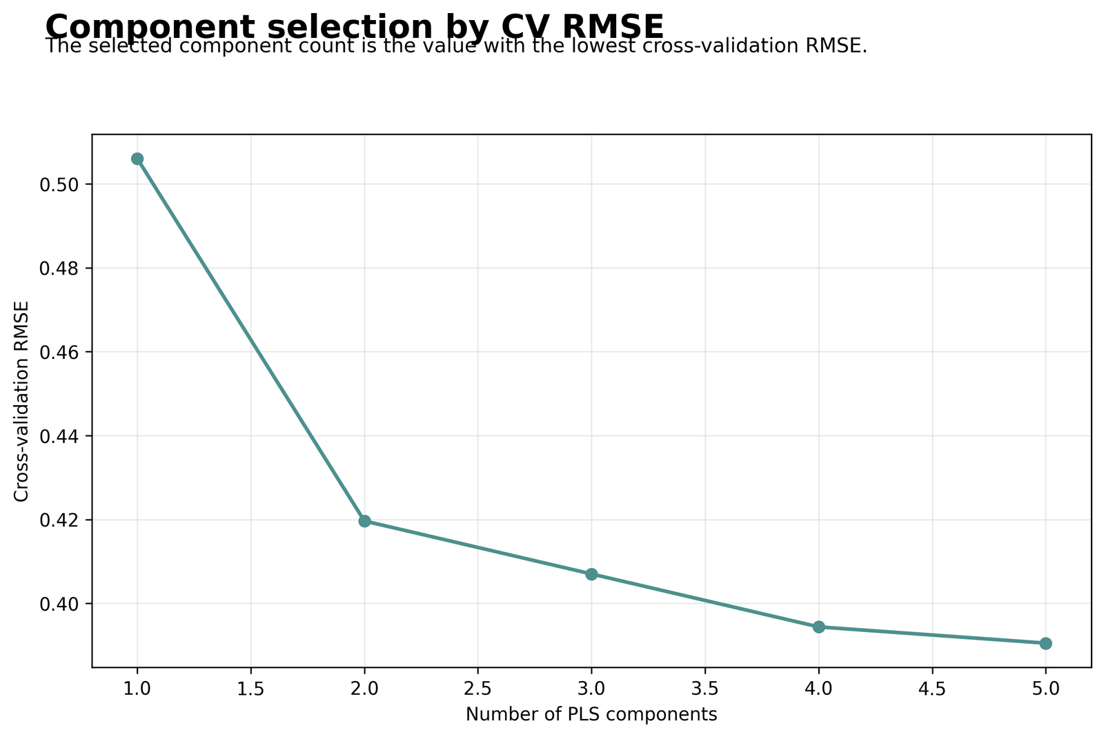
The largest improvement occurs between one and two components. Later components continue to reduce error, but the gains become progressively smaller.
1 component: 0.5060; 2: 0.4196; 3: 0.4070; 4: 0.3944; 5: 0.3905. The corresponding standard deviation at five components is 0.0909.
One component compresses the predictor space too aggressively. Two components recover most of the available predictive structure, while components three through five provide smaller refinements. Five components are selected because they produce the lowest cross-validation RMSE among the evaluated range of one through five.
The cross-validation values are reported on the scaled outcome used during component selection and should not be compared directly with the original-scale RMSE of 1.2442. Testing more components could change the minimum, so the conclusion applies to the evaluated range.
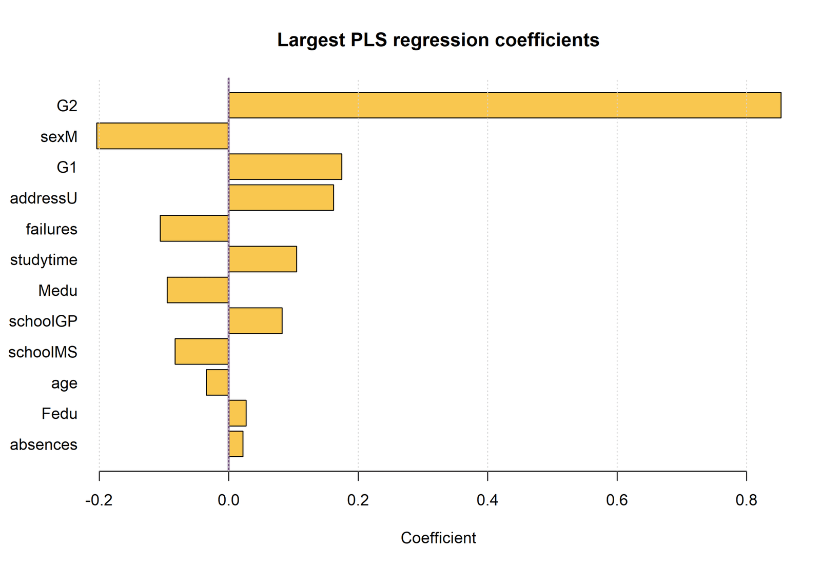
Chart 7: PLS Regression Coefficients
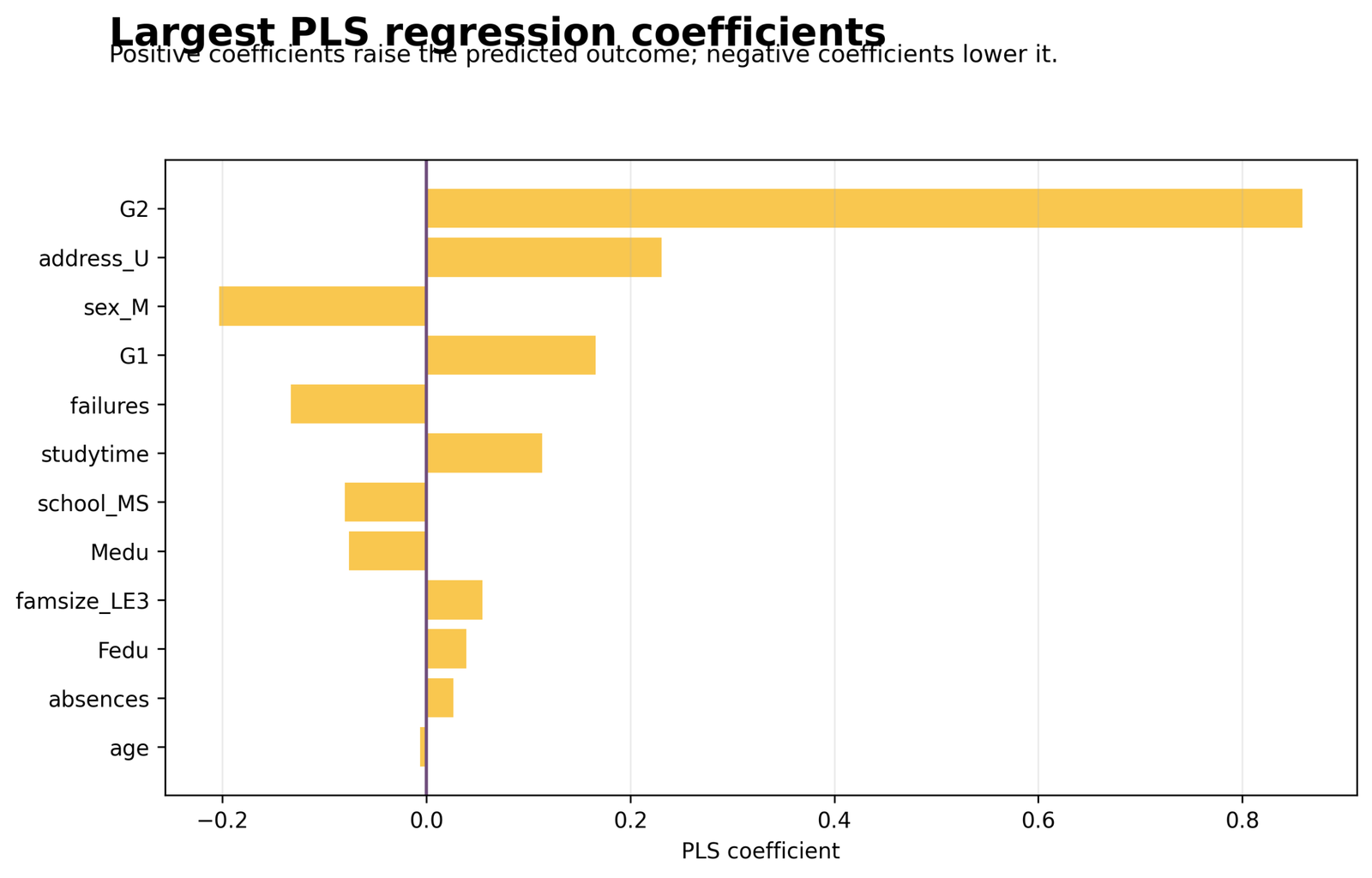
G2 has a much larger positive coefficient than every other predictor. Address_U is the next largest positive coefficient, sex_M the largest negative coefficient, and G1 provides a smaller positive contribution.
G2 = 0.8592; address_U = 0.2308; sex_M = −0.2033; G1 = 0.1657; failures = −0.1330; studytime = 0.1133. All remaining absolute coefficients are below 0.081.
The fitted prediction equation depends mainly on second-period grade. G1, failures, studytime, and several coded group variables make smaller adjustments after the latent-component structure has been reconstructed in the original predictor space.
PLS coefficients are prediction weights, not ordinary least squares significance tests. Their size and direction should be interpreted with scaling, collinearity, VIP scores, and validation performance rather than p-values that were not produced by this model.
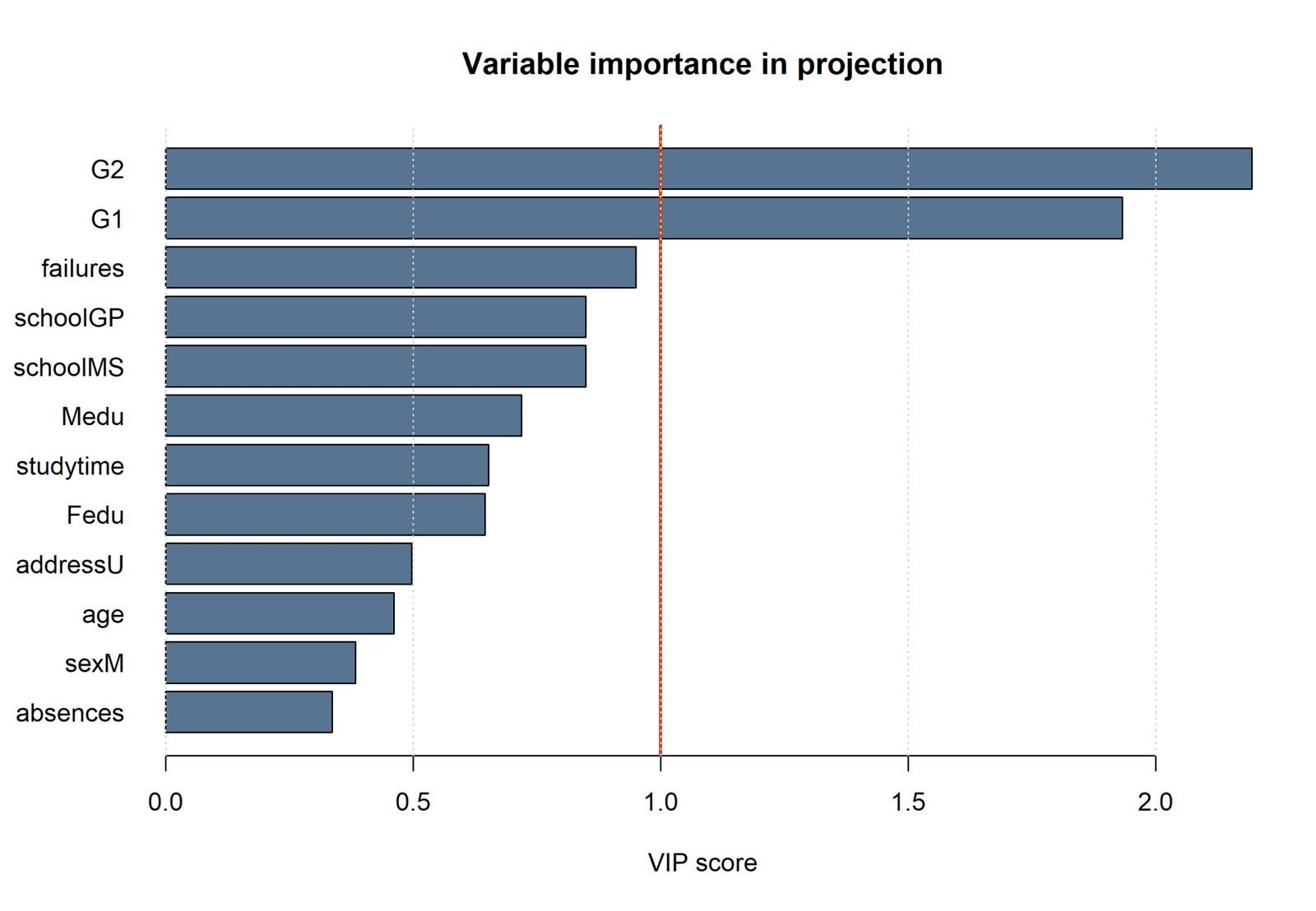
Chart 8: Variable Importance in Projection Scores
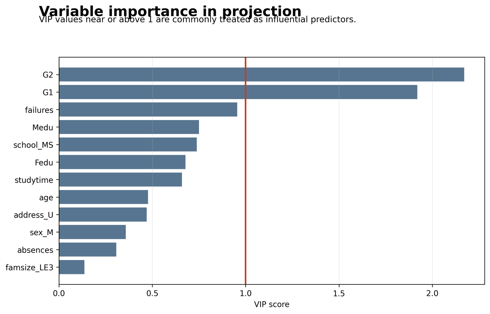
G2 ranks first, G1 second, and failures third. A reference line at VIP = 1 separates the two predictors that exceed the conventional influence threshold.
G2 = 2.1711; G1 = 1.9192; failures = 0.9546; Medu = 0.7508; school_MS = 0.7380; Fedu = 0.6778; studytime = 0.6584. The remaining scores are below 0.50.
Prior academic performance carries most of the information used across the five latent components. Failures contributes meaningfully but sits just below the conventional cutoff. Background and demographic predictors contribute less to the overall latent prediction structure.
VIP is a ranking aid rather than a hypothesis test. A score above 1 suggests influence across the component system, but variable retention should also consider prediction error, subject knowledge, stability across resamples, and the purpose of the model.
Partial Least Squares Regression in R
The complete R chart set covers the outcome, fitted values, residual behavior, latent component structure, component selection, reconstructed coefficients, and variable importance.
R Outcome Distribution
Most final grades fall between about 9 and 15, with the greatest concentration near 12. A smaller group of zero outcomes creates the long lower tail and accounts for several of the model’s largest prediction errors.
R Observed Versus Fitted Values
Predictions follow the agreement line closely across the middle and upper grade ranges. The largest departures occur for students with G3 = 0, whose predictor profiles often generate fitted grades well above zero.
R Residuals Versus Fitted Values
Most residuals remain close to zero, commonly within about two grade points. The diagonal bands result from the integer outcome scale, while the long negative tail reflects substantial overprediction for several zero-grade observations.
R Residual Distribution
Errors are concentrated around zero, but the distribution is asymmetric because a small number of large negative residuals extend farther than the positive tail. Those extreme errors have more influence on RMSE than on MAE.
R Component Score Map
The first component carries the strongest visible grade gradient, with lower outcomes concentrated toward one side and higher outcomes toward the other. The second component adds separation among students with similar first-component scores.
R Cross-Validation RMSE by Components
The largest reduction in error occurs when the model moves from one to two components. Components three through five provide smaller improvements, with five producing the lowest error among the tested component counts.
R Coefficient Importance
G2 has the largest positive prediction coefficient, followed by substantially smaller contributions from the remaining predictors. Negative coefficients indicate downward adjustments to the fitted G3 value after the complete component model is considered.
R Variable Importance in Projection Scores
G2 and G1 rank highest and exceed the commonly used VIP threshold of 1. Failures is close to that threshold, while the demographic and background predictors contribute less to the full latent prediction system.
Partial Least Squares Regression Coefficients and VIP Scores
Reconstructed prediction coefficients
| Predictor | Coefficient | Absolute coefficient | VIP score | Reading |
|---|---|---|---|---|
| G2 | 0.8592 | 0.8592 | 2.1711 | Dominant positive prediction contribution |
| address_U | 0.2308 | 0.2308 | 0.4705 | Positive coefficient but modest component-wide importance |
| sex_M | −0.2033 | 0.2033 | 0.3580 | Negative prediction adjustment with low VIP |
| G1 | 0.1657 | 0.1657 | 1.9192 | Strong component-wide importance despite smaller coefficient than G2 |
| failures | −0.1330 | 0.1330 | 0.9546 | Negative contribution and near-threshold VIP |
| studytime | 0.1133 | 0.1133 | 0.6584 | Smaller positive contribution |
| school_MS | −0.0800 | 0.0800 | 0.7380 | Negative coefficient with moderate VIP |
| Medu | −0.0760 | 0.0760 | 0.7508 | Small reconstructed coefficient |
| famsize_LE3 | 0.0547 | 0.0547 | 0.1365 | Minimal component-wide importance |
| Fedu | 0.0394 | 0.0394 | 0.6778 | Small positive coefficient |
| absences | 0.0264 | 0.0264 | 0.3077 | Small prediction contribution |
| age | −0.0060 | 0.0060 | 0.4770 | Near-zero reconstructed coefficient |
Partial Least Squares Regression coefficients represent the prediction equation after the latent components are translated back into the original design columns. They should not be described as statistically significant or nonsignificant unless a valid resampling or inferential procedure supplies uncertainty estimates.
VIP scores summarize importance across the complete component system. The common threshold of 1 is a convention, not a universal decision boundary. G2 and G1 exceed 1, while failures at 0.9546 may still deserve attention because it lies close to the threshold and has a meaningful negative coefficient.
Component Selection and the Prediction Equation
The displayed equation uses the complete set of twelve reconstructed coefficients. The workbook’s prediction calculator enters the sample means and category proportions and returns a predicted G3 of approximately 11.9060, matching the sample mean outcome.
The intercept is −0.0755. It should not be interpreted as a realistic expected grade for a student with every predictor equal to zero because several zero values are outside the relevant data profile and dummy variables use reference categories.
Five components are retained because cross-validation RMSE decreases from 0.5060 at one component to 0.3905 at five components. The biggest gain occurs by component two; later components refine the prediction more modestly.
Partial Least Squares Regression Diagnostics and Validation
Model diagnostics
- Observed versus fitted agreement
- Residual pattern and tail behavior
- Stability of coefficients and VIP rankings
- Cross-validation error by component count
- Performance on an untouched test set
Workflow safeguards
- Fit scaling inside each training fold
- Keep outcome information out of preprocessing decisions
- Use grouped folds for dependent observations
- Tune components inside nested validation
- Report prediction intervals only when properly estimated
The reported R², RMSE, and MAE describe the fitted sample. Cross-validation provides a stronger estimate of generalization, but the component count and any feature decisions should be selected inside the validation process to avoid optimistic bias.
Partial Least Squares Regression is designed for collinearity, so a high Variance Inflation Factor does not invalidate the latent model in the same way it threatens direct OLS coefficient interpretation. VIF and Tolerance Statistic remain useful for explaining why an ordinary regression alternative may be unstable.
Residual heteroskedasticity can be explored with Breusch-Pagan Test and White Test, although the main evaluation should remain predictive. Outliers and leverage can alter component directions and should be examined through case-level sensitivity analysis.
Partial Least Squares Regression Python, R, SPSS and Excel Workflows
Partial Least Squares Regression Python
Python uses scikit-learn to encode predictors, scale inputs, tune component count, fit PLSRegression, calculate predictions, and derive VIP scores.
Partial Least Squares Regression in R
R packages such as pls, mixOmics, and tidymodels workflows support component tuning, scores, loadings, and resampling. The plsr() function is a common starting point.
Partial Least Squares Regression SPSS
SPSS users can install and run the PLS extension when it is available in their installation. Predictor roles, dummy coding, component count, validation, and output requests should match the model used in Python or R.
Partial Least Squares Regression Excel
The worked Excel file summarizes model fit, coefficients, component selection, predictions, and a live prediction calculator. Excel is useful for reporting and scenario calculations, while model fitting is more dependable in dedicated statistical software.
Partial Least Squares Regression software choices should not change the statistical question. Differences in scaling defaults, cross-validation folds, dummy coding, and algorithm variants can change numerical results and must be documented.
Partial Least Squares Regression Code and Software Steps
Partial Least Squares Regression Python example
import numpy as np
import pandas as pd
from sklearn.cross_decomposition import PLSRegression
from sklearn.model_selection import KFold, cross_val_score
from sklearn.preprocessing import StandardScaler
from sklearn.metrics import mean_squared_error, mean_absolute_error, r2_score

df = pd.read_csv("dataset.csv")

predictors = [
    "G1", "G2", "studytime", "failures", "absences",
    "age", "Medu", "Fedu", "school", "sex", "address", "famsize"
]
X = pd.get_dummies(df[predictors], drop_first=True, dtype=float)
y = df["G3"].to_numpy(dtype=float)

# Component selection on a standardized outcome.
y_scaled = StandardScaler().fit_transform(y.reshape(-1, 1)).ravel()
cv = KFold(n_splits=5, shuffle=True, random_state=42)

cv_rmse = {}
for n_components in range(1, 6):
    model = PLSRegression(n_components=n_components, scale=True)
    scores = cross_val_score(
        model, X, y_scaled,
        cv=cv,
        scoring="neg_root_mean_squared_error"
    )
    cv_rmse[n_components] = -scores.mean()

best_components = min(cv_rmse, key=cv_rmse.get)

final_model = PLSRegression(
    n_components=best_components,
    scale=True
).fit(X, y)

predicted = final_model.predict(X).ravel()
print("R2:", r2_score(y, predicted))
print("RMSE:", mean_squared_error(y, predicted) ** 0.5)
print("MAE:", mean_absolute_error(y, predicted))
Partial Least Squares Regression R code
library(pls)

df <- read.csv("dataset.csv")

fit <- plsr(
  G3 ~ G1 + G2 + studytime + failures + absences +
    age + Medu + Fedu + school + sex + address + famsize,
  data = df,
  ncomp = 5,
  scale = TRUE,
  validation = "CV"
)

summary(fit)
validationplot(fit, val.type = "RMSEP")
predicted <- drop(predict(fit, ncomp = 5))
scores(fit)
loadings(fit)
coef(fit, ncomp = 5)
How to do Partial Least Squares Regression in SPSS
Install the PLS extension supported by the available SPSS version, then specify:
- Dependent variable: G3
- Scale predictors: G1, G2, studytime, failures, absences, age, Medu, Fedu
- Categorical predictors: school, sex, address, famsize
- Maximum components: at least 5
- Selection: cross-validation error
- Output: scores, loadings, coefficients, predictions, residuals, and VIP values when supported
Record the installed extension version and default scaling rules because SPSS PLS syntax and available output can vary by installation.
Partial Least Squares Regression Excel formulas
Prediction from reconstructed coefficients:
=Intercept
 + G1_Input*G1_Coefficient
 + G2_Input*G2_Coefficient
 + Studytime_Input*Studytime_Coefficient
 + Failures_Input*Failures_Coefficient
 + ...

Residual:
=Observed_G3-Predicted_G3

Absolute residual:
=ABS(Residual)

Squared residual:
=Residual^2

RMSE:
=SQRT(AVERAGE(Squared_Residual_Range))

MAE:
=AVERAGE(Absolute_Residual_Range)
Advanced Partial Least Squares Regression Topics
PLS Regression Explained for Beginners
PLS regression replaces a crowded predictor set with a few outcome-focused patterns. Those patterns summarize shared predictor information and retain the parts most useful for predicting the response.
PLS Regression Tutorial Workflow
A complete Partial Least Squares Regression tutorial should cover data preparation, dummy coding, scaling, component tuning, model fitting, coefficient reconstruction, VIP calculation, residual review, and validation on unseen data.
Worked PLS Regression Example
In this PLS regression example, five components explain 85.15% of G3 variation. G2 and G1 dominate the latent prediction structure, while failures is close to the conventional VIP threshold.
Principal components regression vs Partial Least Squares Regression
Principal components regression selects directions that explain X variance. Partial Least Squares Regression selects directions with high X–Y covariance. The response therefore influences the PLS components but not the initial PCR components.
Partial Least Squares vs multiple linear regression
Multiple linear regression estimates original-variable effects directly. PLS regression uses latent components to stabilize prediction when original predictors overlap strongly or the design is high dimensional.
Partial Least Squares Regression vs ordinary least squares
OLS minimizes residual sum of squares in the original predictor space. Partial Least Squares Regression first reduces X to supervised latent dimensions, then performs prediction through that reduced representation.
Scaling Predictors and the Outcome
Scaling prevents predictors with large units from dominating component construction. The scaling operation must be estimated inside each training fold to prevent information leakage.
Interpreting PLS Coefficients
Partial Least Squares Regression coefficients reconstruct the latent model in the original design space. Their signs and magnitudes describe prediction contributions, but they do not automatically include classical inferential uncertainty.
Interpreting VIP Scores
VIP scores combine a variable’s contribution across all selected components, weighted by outcome explanation. Values near or above 1 are often highlighted, but the threshold is conventional rather than a hypothesis test.
Scores and Loadings
Scores locate observations in latent space; loadings describe how the original variables relate to that space. Both are useful for interpretation, clustering, and identifying unusual observations.
R-Squared and Prediction Error
R² = 0.8515 summarizes fitted-sample outcome variation. Adjusted R-Squared using five components is 0.8503, but external or cross-validated prediction remains more important than training fit.
Categorical Predictors in PLS
Categorical predictors enter Partial Least Squares Regression through dummy or contrast coding. Their coefficients depend on the selected reference category and the scaling used for the design matrix.
Non-Normal Data and PLS
Prediction with PLS regression does not require every predictor to be normally distributed. Severe skew, outliers, and nonlinear response patterns can still destabilize components and should be investigated.
Supervised Dimension Reduction
The selected components provide a lower-dimensional supervised representation of the predictor matrix. Five components replace twelve design columns in this worked model.
Latent-Component Regularization
Component truncation acts as a form of regularization because weak directions are excluded. Unlike Lasso or Elastic Net, the method regularizes through latent projection rather than direct coefficient penalties.
Sparse PLS
Sparse Partial Least Squares Regression adds variable selection to component construction. It can improve interpretability in very wide datasets but introduces additional tuning decisions.
Robust PLS
Robust PLS regression reduces the influence of outliers or heavy-tailed observations during component estimation. It is useful when standard PLS scores change substantially after unusual cases are removed.
Kernel PLS
Kernel Partial Least Squares Regression represents nonlinear relationships through a kernel function. Kernel choice and tuning can improve prediction but make interpretation less direct.
Orthogonal PLS
Orthogonal PLS separates predictive variation from structured X variation unrelated to Y. The separation can aid visualization, but validation remains necessary because added model flexibility can overfit.
SIMPLS algorithm
SIMPLS is an alternative algorithm for extracting Partial Least Squares Regression components. Different algorithms can reach equivalent prediction spaces while using different computational procedures.
PLS in Machine Learning
Machine learning workflows treat component count as a hyperparameter and evaluate PLS regression through resampling, pipelines, and an untouched test set.
Scikit-Learn PLSRegression
Scikit-learn provides PLSRegression for Partial Least Squares Regression Python projects. Preprocessing, component tuning, and metric calculation should be placed in a reproducible pipeline.
R Packages for PLS
R implementations include pls, mixOmics, and model interfaces in broader resampling frameworks. Defaults for scaling, validation, and coefficient extraction should be checked.
SPSS PLS Output
Partial Least Squares Regression SPSS output should identify the number of latent factors, fit metrics, predictor weights, loadings, coefficients, and validation method. Available tables depend on the installed extension.
Excel Capabilities and Limitations
Excel can reproduce a fitted prediction equation and summarize results, but deriving stable latent components, resampling, and VIP scores is safer in Python, R, SPSS extensions, MATLAB, Minitab, or specialist software.
Reporting a PLS Model
Report the outcome, design columns, scaling, selected components, cross-validation method, R², RMSE, MAE, coefficients, VIP scores, and residual findings. Use Confidence Interval language only when uncertainty has actually been estimated.
APA-Style Reporting
G2 had the largest reconstructed coefficient, B = 0.859, and the highest VIP score, 2.171. G1 also exceeded the conventional VIP threshold, VIP = 1.919. Failures had a negative coefficient, B = −0.133, and VIP = 0.955.
The report should avoid describing coefficients as statistically significant because the fitted Partial Least Squares Regression output does not provide standard errors or p-values. Validation metrics, coefficient stability, and VIP rankings should be reported as prediction evidence rather than classical hypothesis tests.
Publication Checklist and Common Mistakes
Include
- Outcome and complete predictor list
- Dummy-coding and reference categories
- Scaling procedure
- Candidate and selected component counts
- Cross-validation design
- R², RMSE, and MAE with scales identified
- Coefficients, VIP scores, scores, and loadings where relevant
- Residual and outlier findings
Avoid
- Selecting components from training R²
- Scaling the full dataset before validation
- Treating VIP > 1 as statistical significance
- Calling coefficients causal effects
- Comparing scaled and original-scale RMSE directly
- Using random folds for dependent observations
- Ignoring zero-outcome residuals
Model claims should distinguish prediction from inference and should connect uncertainty to P-Value, Confidence Interval, Effect Size, and Statistical Power only when those concepts are supported by the fitted procedure.
Downloads
Frequently Asked Questions
What is Partial Least Squares Regression?
When to use Partial Least Squares Regression?
How does Partial Least Squares Regression work?
What is the difference between principal component regression and Partial Least Squares Regression?
What is the difference between Partial Least Squares Regression and multiple linear regression?
How many components were selected in this example?
What is the Partial Least Squares Regression R squared?
What is the RMSE of the model?
How do you interpret Partial Least Squares Regression coefficients?
What are VIP scores in Partial Least Squares Regression?
Which variables are most important here?
Can Partial Least Squares Regression use categorical variables?
How do you perform Partial Least Squares Regression Python analysis?
How do you perform Partial Least Squares Regression in R?
How do you do Partial Least Squares Regression in SPSS?
Can Partial Least Squares Regression be done in Excel?
Partial Least Squares Regression Conclusion
Partial Least Squares Regression provides an outcome-focused alternative to ordinary regression and unsupervised principal component regression when predictors contain overlapping information. The method compresses the design into latent components, selects the component count through validation, and reconstructs predictions in the original variable space.
In this example, five components explain 85.15% of G3 variation with RMSE of 1.2442 and MAE of 0.7843. G2 and G1 dominate the latent prediction structure, failures contributes a smaller negative signal, and the remaining variables provide limited additional importance.
The model performs well across the main outcome range, while zero-grade cases produce the largest errors. The most defensible conclusion combines the strong fitted performance with the validation curve, residual pattern, and the distinction between VIP ranking and statistical significance.

