
Lasso Regression: Formula, Interpretation, Python, R, SPSS and Excel Guide
Lasso Regression combines linear prediction with an L1 penalty that can shrink weak coefficients exactly to zero. This complete worked guide uses 649 students, predicts G3 from twelve encoded predictors, explains alpha and lambda selection, interprets every chart, compares Python and R results, and provides reproducible SPSS and Excel teaching workflows.
12 encoded predictors
7 Python charts
8 paired R visuals
Lasso Regression Model Overview
What this model is and when it is used: Lasso Regression is a regularized linear model for a continuous outcome. It is used when the analyst wants prediction, coefficient shrinkage and automatic feature selection in one procedure, especially when candidate predictors are numerous, partially redundant or vulnerable to overfitting. The dependent variable should be continuous for the standard Gaussian form used here, while predictors may be continuous, ordinal, binary or categorical after categorical values are encoded as indicator columns. Lasso Regression minimizes squared prediction error plus the sum of absolute coefficient magnitudes multiplied by a penalty parameter. As the penalty increases, weak coefficients become smaller and some become exactly zero.
Quick Answer: Lasso Regression Results
Python Lasso Regression
The Python workflow selects the penalty using five-fold cross-validation inside 486 training observations and evaluates the final pipeline on 163 held-out observations.
- Alpha = 0.016927
- 10 non-zero predictors
- Test MAE = 0.7253
- Test RMSE = 1.1156
- Test R² = 0.8765
R Lasso Regression
The R workflow uses five-fold cross-validation on all 649 rows and reports both the minimum-error penalty and the simpler one-standard-error penalty.
- lambda.min = 0.054286
- 8 non-zero predictors
- lambda.1se = 0.461293
- 2 non-zero predictors at lambda.1se
- R² = 0.8508 at lambda.min
Table of Contents
- What Lasso Regression is
- How Lasso Regression works
- Variables and coding
- Scaling, splitting and cross-validation
- Results at a glance
- Python chart stories
- R charts with explanation boxes
- Selected coefficients
- Prediction and diagnostics
- Lasso, Ridge, OLS and Elastic Net
- Python, R, SPSS and Excel
- Worked Excel explanation
- Code
- Advanced interpretation
- APA-style reporting
- Publication checklist
- Downloads
- Related guides
- FAQs
What Is Lasso Regression?
Lasso Regression stands for Least Absolute Shrinkage and Selection Operator Regression. It starts with the ordinary squared-error objective and adds an L1 penalty equal to the sum of the absolute coefficient values. The penalty creates a practical distinction from ordinary least squares: Lasso Regression can remove variables from the active model by setting their coefficients exactly to zero.
Lasso Regression is commonly used for continuous-outcome prediction, high-dimensional modeling, sparse feature selection and situations where a simpler model is preferred to one that retains every candidate variable. It is especially useful when the research goal is to build a compact predictive equation rather than test a separate null hypothesis for every coefficient.
Lasso Regression does not automatically prove that a retained variable is causally important, and a zero coefficient does not prove that the variable is unrelated to the outcome in the population. Selection depends on the observed sample, penalty grid, cross-validation folds, scaling, coding and correlation among predictors.
How Lasso Regression Works
Encode categorical variables and standardize numeric scales inside the modeling pipeline.
Use cross-validation to compare alpha or lambda values.
Retain non-zero coefficients and evaluate predictions.
The first term measures squared prediction error. The second term is the L1 penalty. In Python, the penalty is commonly called alpha; in R glmnet output, it is commonly called lambda. The symbols differ by software convention, but both control the strength of shrinkage in this Lasso Regression analysis.
When the penalty is very small, Lasso Regression approaches an unpenalized regression and retains more predictors. When the penalty is large, coefficients move toward zero and prediction may deteriorate because useful information is removed. Cross-validation estimates the penalty that best balances these competing effects.
The L1 geometry is responsible for exact zeros. The optimization solution often touches a corner of the constrained coefficient region, producing a sparse active set. This makes Lasso Regression different from Ridge, which shrinks all slopes but ordinarily retains all predictors.
Lasso Regression Variables Used and Coding
| Variable | Role | Definition | Model type |
|---|---|---|---|
| G3 | Outcome | Final grade from 0 to 19. | Continuous |
| G1 | Predictor | First-period grade. | Continuous |
| G2 | Predictor | Second-period grade. | Continuous |
| studytime | Predictor | Weekly study-time category. | Ordinal |
| failures | Predictor | Number of previous class failures. | Ordinal/count |
| absences | Predictor | School absence count. | Count |
| age | Predictor | Student age in years. | Continuous |
| Medu | Predictor | Mother’s education level. | Ordinal |
| Fedu | Predictor | Father’s education level. | Ordinal |
| school_MS | Encoded predictor | MS compared with GP. | Binary indicator |
| sex_M | Encoded predictor | Male compared with female. | Binary indicator |
| address_U | Encoded predictor | Urban compared with rural. | Binary indicator |
| famsize_LE3 | Encoded predictor | Family size ≤3 compared with GT3. | Binary indicator |
Lasso Regression Data Preparation, Scaling and Validation
The model begins with 649 rows and 33 original columns. The selected outcome is G3. Eight numeric predictors and four categorical contrasts create 12 encoded predictor columns. The Python workflow divides the data into 486 training rows and 163 held-out test rows, while the R report fits and summarizes the cross-validated model using all 649 rows.
Scaling is essential because the L1 penalty acts directly on coefficient magnitudes. Without standardization, a variable measured on a wide numeric scale can receive a small coefficient merely because of its units, while a binary variable can receive a different penalty effect. A defensible Lasso Regression pipeline learns means and standard deviations from training data only and applies the learned transformation to validation or test data.
Dummy-variable creation, missing-data handling and scaling should occur inside each training fold. Preprocessing the full dataset before cross-validation leaks information from validation folds and makes prediction error too optimistic. The same principle applies to imputation and any outcome-informed feature selection.
Five-fold cross-validation means the training sample is divided into five parts. Four parts fit the Lasso Regression model and the remaining part measures error. The process rotates through all five parts and averages the errors for each candidate penalty. The selected penalty is then used to refit the model on the complete training sample.
Lasso Regression Results at a Glance
Selected with five-fold CV
Lower than Ridge and OLS
163 held-out rows
Eight active predictors
Two active predictors
All 649 rows
| Comparison item | Python Lasso Regression | R Lasso Regression | Interpretation |
|---|---|---|---|
| Sample/evaluation | Train 486; test 163 | All 649 rows | Python reports held-out performance; R reports fitted all-data performance. |
| Penalty rule | alpha = 0.016927 | lambda.min = 0.054286 | Both are chosen by five-fold cross-validation but use different grids and implementations. |
| Simpler rule | Not separately reported | lambda.1se = 0.461293 | The one-standard-error rule retains only two predictors. |
| Non-zero predictors | 10 | 8 at lambda.min; 2 at lambda.1se | Different selection counts are expected when penalty rules and scaling differ. |
| RMSE | 1.1156 on test | 1.246956 at lambda.min | The metrics are not directly comparable because the evaluation samples differ. |
| MAE | 0.7253 on test | 0.775720 at lambda.min | Lower values indicate smaller average prediction errors. |
| R² | 0.8765 on test | 0.850793 at lambda.min | The Python test split happened to produce stronger performance than the R all-data fitted value. |
| Strongest retained term | G2 standardized = 2.4765 | G2 = 0.877895 | The numerical scales differ, but both implementations identify G2 as dominant. |
Download the Lasso Regression Outputs
The same resources appear again in the complete Downloads section.
Python Lasso Regression Chart Stories
Every Python figure is followed by four interpretation boxes so that Lasso Regression charts are treated as analytical evidence rather than decoration.
Python Chart 1: Lasso Regression Outcome Distribution
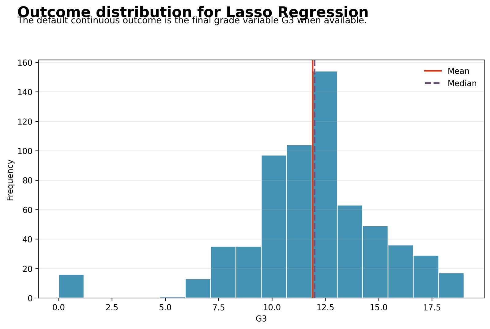
This histogram establishes the continuous outcome that the Python Lasso Regression pipeline predicts. It shows the central grade concentration, the lower tail and the small zero-grade group before any regularization is applied.
The sample contains 649 rows. G3 has mean approximately 11.906, median 12, standard deviation approximately 3.231, and range 0–19. About 16 observations occur at G3 = 0.
The outcome is concentrated around grades 10–13 but is not perfectly symmetric because the isolated zero group creates a longer lower tail. Lasso Regression still models the conditional mean as continuous, so residual and influence checks remain important.
Compare the histogram with observed-versus-predicted and residual charts. Investigate zero-grade cases rather than deleting them automatically, because they may represent valid difficult-to-predict outcomes.
Python Chart 2: Lasso Regression Cross-Validation MSE
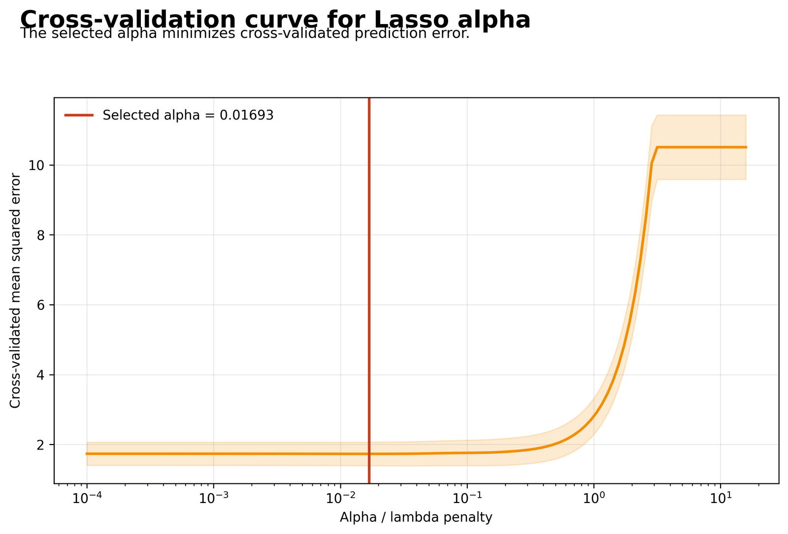
The curve displays mean cross-validated squared error across a logarithmic grid of penalty strengths. The vertical line marks the alpha selected inside the training data.
The Python workflow uses five folds and selects alpha = 0.016927. At this penalty, Lasso Regression retains 10 of 12 encoded predictors.
Very small penalties behave similarly to an almost unregularized model, while large penalties sharply increase prediction error by overshrinking useful coefficients. The selected alpha lies near the broad low-error region.
Repeat the full pipeline with repeated cross-validation or nested cross-validation when penalty-selection stability is important. Keep scaling and dummy coding inside the training workflow.
Python Chart 3: Lasso Regression Coefficient Path
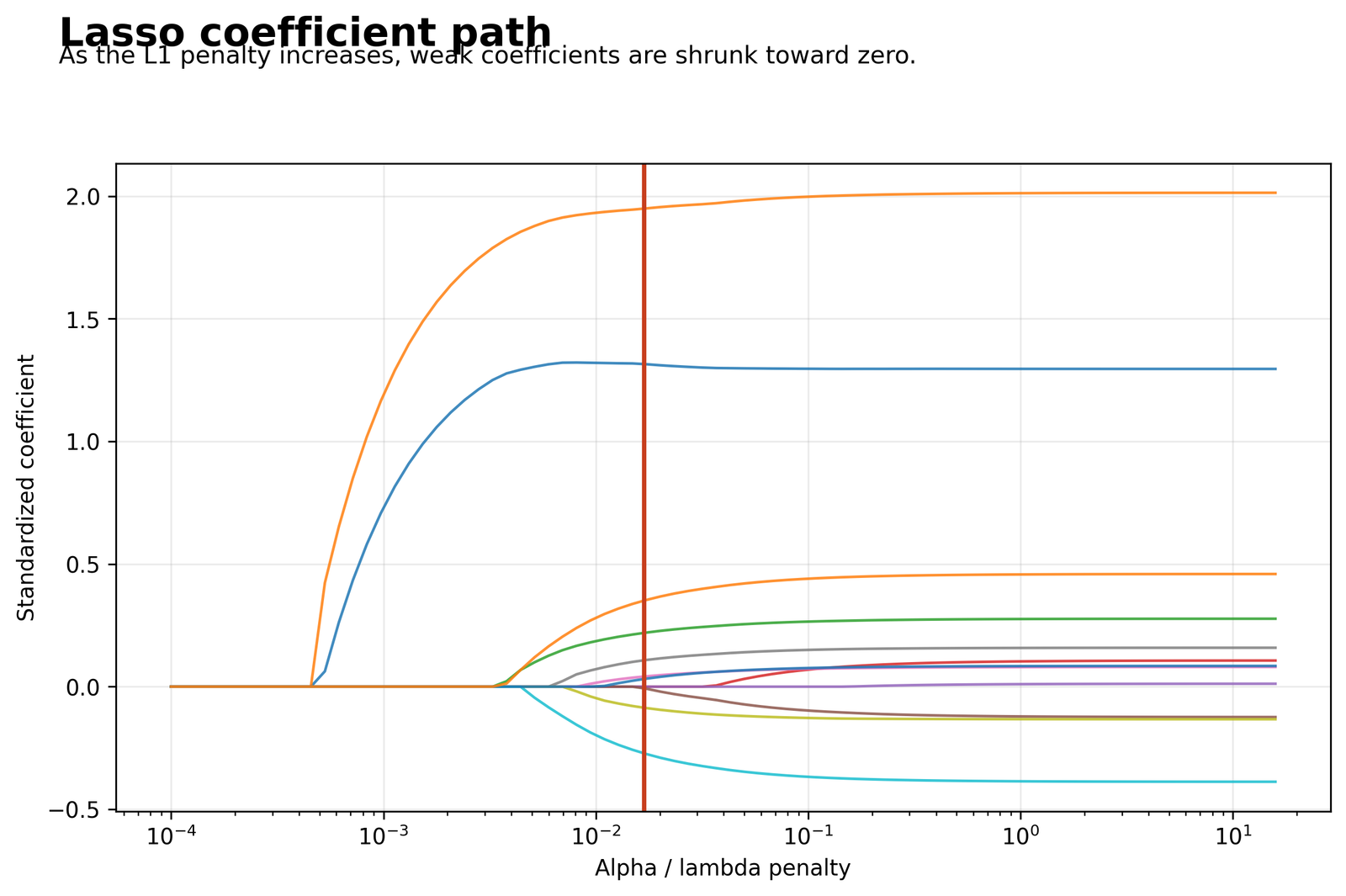
Every line represents one encoded predictor. Moving toward stronger regularization increases the L1 constraint, causing weak paths to reach zero earlier than strong paths.
The selected vertical line is near alpha = 0.01693. G2 and G1 remain the dominant positive paths, while school_MS, Medu, failures and sex_M remain negative at the chosen penalty.
Lasso Regression performs continuous shrinkage and discrete selection at the same time. Variables with zero coefficients are excluded from the active prediction equation at the selected penalty.
Do not interpret entry order as a p-value ranking. Examine coefficient stability across resamples, especially when predictors such as G1 and G2 are correlated.
Python Chart 4: Predictors Selected by Lasso Regression
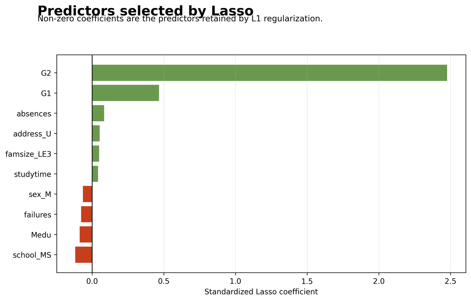
The horizontal bars display the selected standardized coefficients. Positive bars increase predicted G3; negative bars decrease predicted G3, conditional on the remaining retained variables.
G2 = 2.4765, G1 = 0.4670, school_MS = -0.1176, Medu = -0.0867, absences = 0.0834, failures = -0.0766, sex_M = -0.0640, address_U = 0.0532, famsize_LE3 = 0.0485 and studytime = 0.0412. Fedu and age are zero.
G2 is by far the strongest standardized predictor, followed by G1. The smaller bars represent weak conditional contributions after the strongest grade variables are included.
Interpret coefficient direction and relative standardized magnitude, but avoid ordinary t-test language. Penalized coefficients are biased toward zero and were selected through cross-validation.
Python Chart 5: Lasso Regression Observed vs Predicted
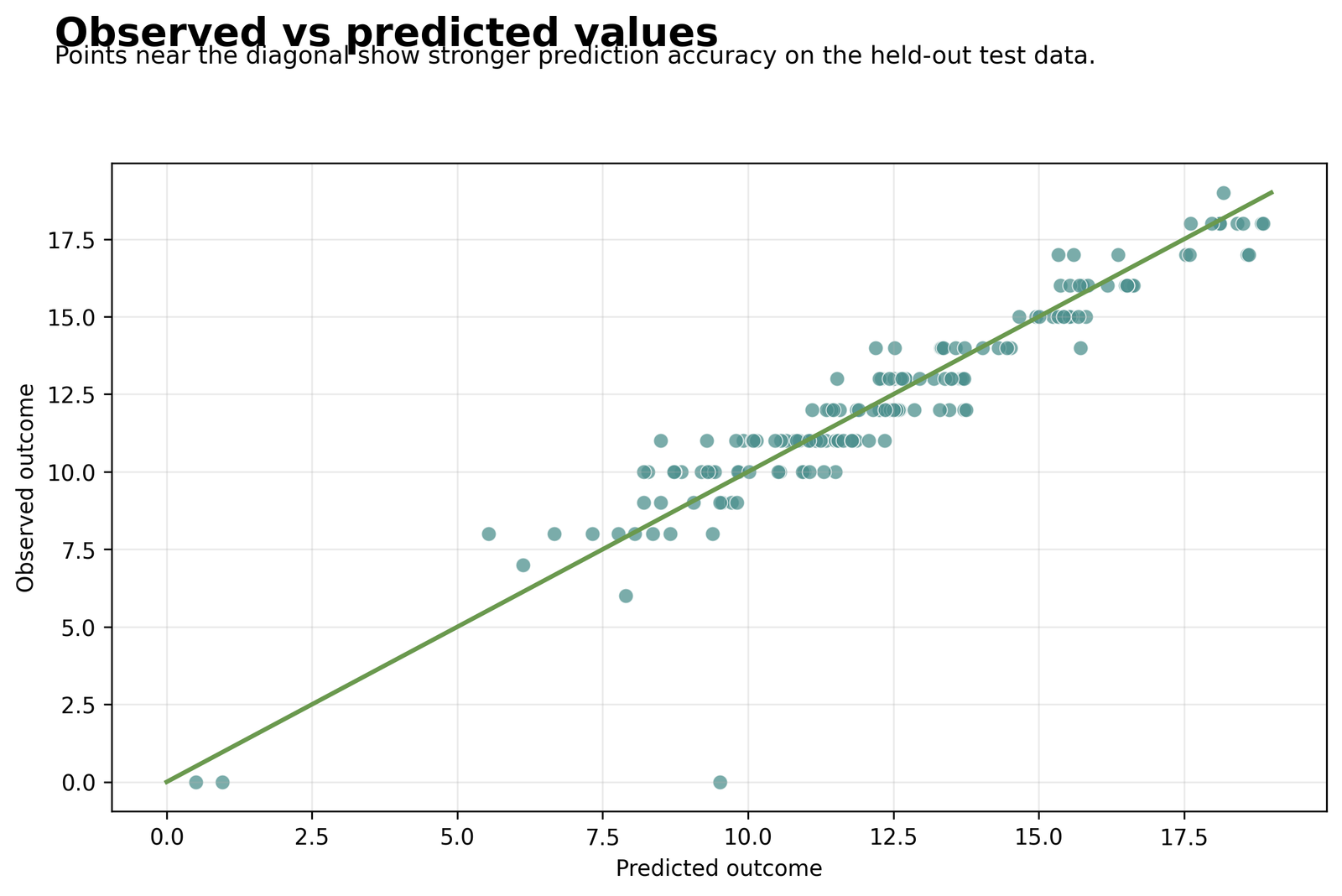
Points near the 45-degree line indicate accurate prediction. Horizontal bands occur because observed G3 is integer-valued while predictions are continuous.
The held-out test sample contains 163 observations. Test RMSE is 1.1156, MAE is 0.7253, and R² is 0.8765.
The model predicts the central and upper grade range closely, but several G3 = 0 cases receive much larger fitted values. The high R² does not eliminate large individual errors.
Report both average error and difficult cases. Compare performance with repeated splits because one favorable holdout can produce an R² above the training value.
Python Chart 6: Lasso Regression Residuals vs Predicted
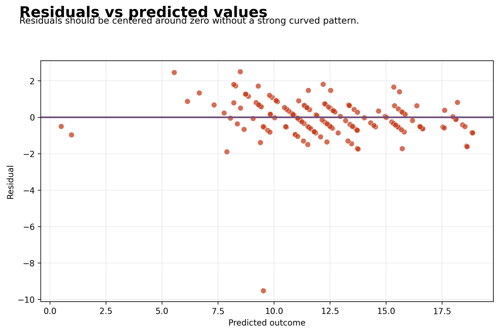
The residual plot checks whether errors remain centered around zero across the prediction range and identifies extreme underprediction or overprediction.
Most residuals lie approximately between -2 and +2.5. One extreme negative residual is close to -9.5, corresponding to a zero observed grade predicted near 9.5.
There is no dominant smooth curve across the main cloud, but the extreme lower tail shows that Lasso Regression cannot explain every unusual grade outcome from the available predictors.
Use studentized residuals, leverage and influence diagnostics on an unpenalized diagnostic refit or a carefully designed regularized diagnostic workflow. Confirm data quality for extreme cases.
Python Chart 7: Lasso Regression RMSE Comparison
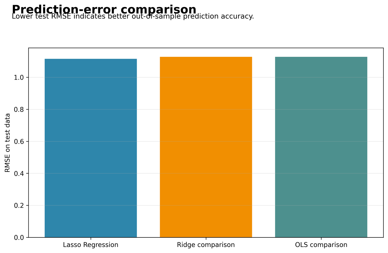
The bars provide a direct predictive comparison using the same held-out test observations and the same encoded predictor set.
Test RMSE is 1.1156 for Lasso Regression, 1.1277 for Ridge and 1.1278 for OLS. Corresponding test R² values are 0.8765, 0.8738 and 0.8738.
Lasso Regression has the lowest test RMSE in this split while using only 10 predictors. The predictive advantage is modest, so the practical benefit is mainly the combination of sparsity and slightly better test error.
Repeat the comparison over multiple resamples. Choose the final method using prediction, stability, interpretability and the cost of retaining extra variables.
R Lasso Regression Charts: Two Charts Followed by Two Explanation Boxes
Each group presents two R Lasso Regression visuals first. Two matching explanation boxes appear directly underneath in the same left-to-right order. On mobile devices, every chart stacks with its correct explanation.
R Chart 1: Lasso Regression Outcome Distribution
R uses all 649 observations with G3 ranging from 0 to 19, mean approximately 11.906 and median 12.
R Chart 2: Lasso Regression Cross-Validation Curve
lambda.min = 0.054286 and lambda.1se = 0.461293. The first retains 8 predictors; the second retains only 2.
R Chart 3: Lasso Regression Coefficient Path
G2 remains the dominant positive path. G1, failures, schoolMS and sexM remain visible as the penalty relaxes, while weaker terms enter later.
R Chart 4: Predictors Selected by Lasso Regression
G2 = 0.877895, failures = -0.145346, G1 = 0.125335, schoolMS = -0.122469, sexM = -0.114708, addressU = 0.022050, studytime = 0.021098 and absences = 0.005108.
R Chart 5: Lasso Regression Observed vs Predicted
At lambda.min, RMSE is 1.246956, MAE is 0.775720, and R² is 0.850793 across 649 observations.
R Chart 6: Lasso Regression Residuals vs Predicted
Most residuals are near -2 to +2, with a positive extreme above +5 and negative residuals approaching -9.
The model active predictors
R Chart 7: Lasso Regression RMSE Comparison
RMSE is 1.246956 for lambda.min, 1.347221 for lambda.1se and 1.239885 for OLS.
R Chart 8: Lasso Regression Sparsity Comparison
lambda.min retains 8 predictors, lambda.1se retains 2 predictors, and OLS uses all 12 encoded predictors.
Lasso Regression Coefficients and Feature Selection
Lasso coefficients must be interpreted in the context of scaling and the selected penalty. The Python report ranks standardized coefficients, while the R report displays coefficients from its model matrix at lambda.min. The signs and selected-variable patterns are comparable, but the numerical magnitudes should not be treated as if they share the same unit.
| Predictor | Python coefficient | Python status | R coefficient | R status | Interpretation |
|---|---|---|---|---|---|
| G2 | 2.4765 | Selected | 0.877895 | Selected | Strong positive predictor in both implementations. |
| G1 | 0.4670 | Selected | 0.125335 | Selected | Smaller positive prior-grade contribution. |
| school_MS / schoolMS | -0.1176 | Selected | -0.122469 | Selected | Negative conditional school contrast. |
| sex_M / sexM | -0.0640 | Selected | -0.114708 | Selected | Negative conditional sex contrast. |
| address_U / addressU | 0.0532 | Selected | 0.022050 | Selected | Small positive address contrast. |
| studytime | 0.0412 | Selected | 0.021098 | Selected | Small positive retained coefficient. |
| absences | 0.0834 | Selected | 0.005108 | Selected | Positive but small after adjustment. |
| failures | -0.0766 | Selected | -0.145346 | Selected | Negative retained predictor. |
| Medu | -0.0867 | Selected | 0 | Zero | Selection differs across penalty and scaling choices. |
| famsize_LE3 | 0.0485 | Selected | 0 | Zero | Selected only in the Python model. |
| Fedu | 0 | Zero | 0 | Zero | Removed in both implementations. |
| age | -0.0000 | Zero | 0 | Zero | Removed in both implementations. |
Python Lasso Regression active set
Ten predictors remain active. G2 and G1 dominate, while school_MS, Medu, failures and sex_M are negative. Fedu and age are removed.
R Lasso Regression active set
Eight predictors remain active at lambda.min. Age, Medu, Fedu and famsizeLE3 are removed. At lambda.1se, only G2 and G1 remain.
Lasso Regression Prediction, Residuals and Diagnostic Interpretation
Prediction evidence
- Python held-out RMSE = 1.1156
- Python held-out MAE = 0.7253
- Python held-out R² = 0.8765
- R all-data RMSE = 1.246956
- R all-data R² = 0.850793
Diagnostic evidence
- Most residuals are within about two grade points.
- Several zero-grade cases are strongly overpredicted.
- Residual bands reflect integer-valued G3.
- No dominant smooth curve appears in the central cloud.
- Extreme cases need influence and data-quality review.
Lasso Regression is optimized for prediction under a penalty, but it still relies on a linear predictor. A residual plot can reveal curvature, changing variance and extreme observations. The available plots show a generally centered main cloud with a long negative tail caused by unexpectedly low final grades.
Because the Python metrics come from one held-out split, they are closer to independent prediction evidence than the all-data R metrics. However, a single split can be unusually easy or difficult. Repeated cross-validation or nested cross-validation provides a more stable estimate of how The penalized model will perform on future students.
Traditional leverage and Cook’s distance formulas are defined for ordinary least squares. For a practical diagnostic sensitivity analysis, analysts can refit OLS on the active variables, inspect influence, and then verify whether the The L1 model selection and test error remain stable when unusual observations are investigated.
Lasso Regression vs Ridge, OLS and Elastic Net
Held-out Python comparison
- The model RMSE = 1.1156
- Ridge RMSE = 1.1277
- OLS RMSE = 1.1278
- Lasso retains 10 predictors
- Ridge and OLS retain all 12
All-data R comparison
- lambda.min RMSE = 1.246956
- lambda.1se RMSE = 1.347221
- OLS RMSE = 1.239885
- lambda.min retains 8 predictors
- lambda.1se retains 2 predictors
OLS minimizes training squared error without a coefficient penalty. It is useful when the number of predictors is modest, multicollinearity is manageable and coefficient inference is the main goal. The penalized model accepts biased coefficients to reduce variance and create a sparse equation.
Ridge applies an L2 penalty and usually keeps every predictor. It is often preferred when many correlated variables each carry some information and removing one arbitrary member of a correlated group would be undesirable. Lasso Regression is preferred when exact feature selection and a compact model are important.
Elastic Net Regression combines L1 and L2 penalties. It can retain groups of correlated variables more smoothly than The L1 model while still producing some zeros. When G1 and G2 or other predictors are strongly correlated, Elastic Net is an important sensitivity analysis.
Lasso Regression in Python, R, SPSS and Excel
Python Lasso Regression
Use a pipeline with one-hot encoding, scaling and LassoCV. Select alpha inside the training data, refit, and evaluate the untouched test sample.
- Five-fold alpha selection
- Train/test separation
- Coefficient path and selected terms
- Held-out RMSE, MAE and R²
R Lasso Regression
Use model.matrix and cv.glmnet with alpha = 1. Report lambda.min and lambda.1se because they answer different prediction-versus-simplicity questions.
- Minimum-error penalty
- One-standard-error penalty
- Coefficient path
- Active-set comparison
SPSS Lasso Regression Workflow
SPSS installations differ in native regularization support. A reproducible approach prepares the same encoded dataset and runs Python integration or an extension that supports cross-validated L1 regression.
- Preserve G3 and encoded predictors
- Standardize inside resampling
- Export selected penalty and coefficients
- Save SAV, SPV and PDF outputs
Excel Lasso Regression Teaching File
Excel demonstrates the objective function, L1 penalty and reporting logic. The true cross-validated coefficient estimates should come from Python or R.
- Dataset preparation
- Worked penalized objective
- Coefficient report template
- Model reporting checklist
Lasso Regression Worked Excel File Explained
The Excel workbook is organized into README, Data_Setup, Lasso_Objective, Coefficient_Report, Model_Report and Output_Checklist sheets. It teaches the structure of The L1 model without pretending that a small formula demonstration replaces a cross-validated optimizer.
The Data_Setup sheet names G3 as the continuous outcome and lists G1, G2, studytime, failures, absences and selected dummy-coded categories. The Lasso_Objective sheet uses five example observations, two standardized predictors, an intercept of 10, coefficients of 1.2 and 0.5, and a lambda value of 0.25.
For the five-row illustration, the squared-error sum is 31.1266. The absolute coefficient sum is 1.7. Multiplying the L1 norm by lambda gives 0.425, so the displayed penalized objective is 31.5516. The illustrative RMSE is 2.4951.
The Coefficient_Report sheet is a template for importing final Python or R values. It distinguishes coefficient magnitude, selection status, direction and rank. The Model_Report sheet prompts the analyst to report the selected penalty, number of retained predictors, RMSE, MAE, R² and residual pattern.
The Excel workbook is most useful for teaching why stronger penalties increase the cost assigned to non-zero coefficients. It also clarifies why standardization matters: the L1 penalty acts on numerical coefficient magnitudes, so variables measured in different units must be placed on a comparable scale.
Lasso Regression Code: Expand the Software You Need
Python Lasso pipeline
import pandas as pd
from sklearn.compose import ColumnTransformer
from sklearn.impute import SimpleImputer
from sklearn.linear_model import LassoCV
from sklearn.metrics import mean_absolute_error, mean_squared_error, r2_score
from sklearn.model_selection import train_test_split
from sklearn.pipeline import Pipeline
from sklearn.preprocessing import OneHotEncoder, StandardScaler

df = pd.read_csv("dataset.csv")

y = df["G3"]
numeric = ["G1", "G2", "studytime", "failures",
           "absences", "age", "Medu", "Fedu"]
categorical = ["school", "sex", "address", "famsize"]
X = df[numeric + categorical]

X_train, X_test, y_train, y_test = train_test_split(
    X, y, test_size=0.251, random_state=42
)

numeric_pipe = Pipeline([
    ("imputer", SimpleImputer(strategy="median")),
    ("scaler", StandardScaler()),
])

categorical_pipe = Pipeline([
    ("imputer", SimpleImputer(strategy="most_frequent")),
    ("encoder", OneHotEncoder(drop="first", handle_unknown="ignore")),
])

preprocessor = ColumnTransformer([
    ("numeric", numeric_pipe, numeric),
    ("categorical", categorical_pipe, categorical),
])

model = Pipeline([
    ("preprocess", preprocessor),
    ("lasso", LassoCV(cv=5, max_iter=100000, random_state=42)),
])

model.fit(X_train, y_train)
pred = model.predict(X_test)

rmse = mean_squared_error(y_test, pred) ** 0.5
mae = mean_absolute_error(y_test, pred)
r2 = r2_score(y_test, pred)

print(model.named_steps["lasso"].alpha_)
print(rmse, mae, r2)
R The penalized model with glmnet
library(glmnet)

df <- read.csv("dataset.csv", stringsAsFactors = TRUE)

formula <- G3 ~ G1 + G2 + studytime + failures +
  absences + age + Medu + Fedu +
  school + sex + address + famsize

x <- model.matrix(formula, data = df)[, -1]
y <- df$G3

set.seed(42)
cv_fit <- cv.glmnet(
  x = x,
  y = y,
  alpha = 1,
  nfolds = 5,
  standardize = TRUE,
  family = "gaussian"
)

lambda_min <- cv_fit$lambda.min
lambda_1se <- cv_fit$lambda.1se

coef_min <- coef(cv_fit, s = "lambda.min")
coef_1se <- coef(cv_fit, s = "lambda.1se")

pred_min <- as.numeric(
  predict(cv_fit, newx = x, s = "lambda.min")
)

rmse <- sqrt(mean((y - pred_min)^2))
mae <- mean(abs(y - pred_min))
r2 <- 1 - sum((y - pred_min)^2) / sum((y - mean(y))^2)

print(lambda_min)
print(lambda_1se)
print(coef_min)
print(c(rmse = rmse, mae = mae, r_squared = r2))
SPSS preparation and Python integration pattern
* Prepare and save the analysis dataset.
GET DATA
 /TYPE=TXT
 /FILE='D:\DATA ANALYSIS\H Regression Tests and Models\The L1 model\dataset.csv'
 /ENCODING='UTF8'
 /DELCASE=LINE
 /DELIMITERS=","
 /ARRANGEMENT=DELIMITED
 /FIRSTCASE=2
 /IMPORTCASE=ALL.

SAVE OUTFILE=
 'D:\DATA ANALYSIS\H Regression Tests and Models\The model\SPSS_Output\sav\Lasso-Regression-data.sav'.

* Use BEGIN PROGRAM PYTHON to run a compatible L1 workflow
  when the required Python packages are available.

OUTPUT SAVE
 /OUTFILE=
 'D:\DATA ANALYSIS\H Regression Tests and Models\Lasso\SPSS_Output\spv\Lasso-Regression-SPSS-Output.spv'.

OUTPUT EXPORT
 /CONTENTS EXPORT=ALL LAYERS=PRINTSETTING MODELVIEWS=PRINTSETTING
 /PDF DOCUMENTFILE=
 'D:\DATA ANALYSIS\H Regression Tests and Models\The penalized model\SPSS_Output\pdf\Lasso-Regression-SPSS-Output.pdf'.
Excel Lasso Regression formulas
Predicted Y:
=Intercept + Beta_X1*X1_Standardized + Beta_X2*X2_Standardized

Residual:
=Observed_Y-Predicted_Y

Squared error:
=Residual^2

SSE:
=SUM(Squared_Error_Range)

L1 norm:
=ABS(Beta_X1)+ABS(Beta_X2)+...

Penalized objective:
=SSE + Lambda*L1_Norm

RMSE:
=SQRT(AVERAGE(Squared_Error_Range))

Selected predictor:
=IF(ABS(Coefficient)>0,"Selected","Shrunk to zero")
Advanced Lasso Regression Interpretation and Extensions
The main reading path remains compact. Expand only the The L1 model topics needed for the study, report or software workflow.
How The model balances bias and variance
- Lasso accepts systematic shrinkage bias so that estimated coefficients can vary less from sample to sample.
- When ordinary coefficients are noisy, a small amount of bias can improve new-case prediction.
- The correct penalty depends on validation evidence rather than a universal alpha value.
How The penalized model handles irrelevant predictors
- An irrelevant predictor tends to receive a coefficient near zero across the penalty path.
- At the selected penalty, The L1 model can remove the predictor completely.
- Removal should still be checked across resamples because one sample can make a weak variable appear useful.
Why Lasso Regression needs a fixed prediction target
- The penalty must be selected for a clearly defined outcome and future-use setting.
- A model tuned for G3 prediction cannot automatically be reused for pass/fail classification.
- The loss function and evaluation metrics must match the prediction target.
How The model affects interpretability
- A sparse active set is easier to describe than a model containing every available variable.
- Shrinkage complicates direct coefficient inference, so interpretability gains are mainly structural and predictive.
- Report the selected variables together with the penalty and validation design.
Why Lasso should be compared with simple baselines
- A complex regularized workflow should outperform or simplify a reasonable baseline.
- The article compares The penalized model with OLS and Ridge using the same encoded candidates.
- The small Python error advantage supports the sparse model, but repeated validation remains necessary.
How The L1 model treats the intercept
- The intercept is usually not penalized.
- Centering and standardization allow the intercept to represent the expected outcome near average numeric predictor values and reference categories.
- The intercept should be transformed back appropriately when presenting predictions in original units.
How The model predictions are transformed back
- The preprocessing pipeline standardizes predictors but leaves G3 in grade units.
- Predictions therefore remain interpretable on the 0–19 grade scale.
- If the outcome were transformed, inverse transformation would be required before calculating practical errors.
How Lasso can be audited
- Audit the exact input columns, reference categories, active coefficients and prediction rows.
- Recalculate RMSE, MAE and R² from exported observed and predicted values.
- A reproducible audit makes Lasso Regression results easier to verify across software.
Why The penalized model coefficients are biased
- The L1 penalty deliberately pulls coefficients toward zero, so the estimates are biased relative to OLS.
- The potential benefit is lower variance, better prediction and a smaller active set.
- A coefficient should be interpreted as a penalized prediction weight at the selected penalty.
The L1 model and multicollinearity
- Correlated predictors compete to explain similar variation.
- The model may select one member of a correlated group and shrink another to zero.
- Selection can therefore be unstable even when prediction remains stable; compare with Elastic Net.
Why standardization changes Lasso
- The L1 penalty is applied to coefficient magnitude.
- Without scaling, predictor units affect how expensive a coefficient is under the penalty.
- Fit scaling inside training folds to avoid information leakage.
Alpha in Python and lambda in R
- Both values control penalty strength in this article.
- Numerical values are not expected to match because software uses different objective scaling and grids.
- Report the software, function, preprocessing and selected value together.
lambda.min versus lambda.1se
- lambda.min targets the lowest estimated cross-validation error.
- lambda.1se chooses the strongest penalty whose error is within one standard error of the minimum.
- The one-standard-error rule often gives a simpler model with slightly worse prediction.
Feature selection stability
- Repeat cross-validation with different fold assignments.
- Record how often each predictor has a non-zero coefficient.
- Stable prediction with unstable selection should be reported honestly.
Bootstrap selection frequencies
- Resample observations, refit the complete pipeline and record active predictors.
- High selection frequency supports robustness, but it is not an ordinary confidence level.
- Use cluster-aware resampling when observations are grouped.
Post-selection inference
- Ordinary OLS p-values calculated after data-driven selection ignore the selection process.
- Selective-inference or sample-splitting methods are needed for formal post-selection claims.
- For a predictive article, emphasize error, stability and coefficient direction.
The penalized model with correlated G1 and G2
- Both prior grades remain active in Python and R, indicating distinct predictive information.
- Their coefficients are conditional on each other and on the remaining active variables.
- Elastic Net can test whether grouped retention improves stability.
Why G2 is dominant
- G2 is temporally close to G3 and strongly predictive.
- Python gives the largest standardized coefficient to G2, and R gives it the largest active coefficient.
- Dominance in prediction does not by itself establish causation.
Why age and Fedu become zero
- At the selected penalties, their conditional predictive contribution is insufficient to justify a non-zero coefficient.
- Zero does not mean the variables have no bivariate relationship with G3.
- Selection can change under a different sample, penalty or feature set.
Why Medu differs between Python and R
- Python retains Medu with a small negative standardized coefficient, while R sets it to zero at lambda.min.
- Different preprocessing, coefficient scales, grids and evaluation designs can move a weak term across the zero boundary.
- The disagreement is evidence that Medu selection is not highly stable.
Interpreting dummy-variable coefficients
- school_MS compares MS with GP, sex_M compares male with female, address_U compares urban with rural and famsize_LE3 compares smaller with larger families.
- A coefficient is conditional on all other active predictors.
- Changing the reference level changes the displayed contrast but not fitted predictions.
Train-test performance variation
- Python test R² exceeds training R² in this split.
- This can occur by chance when the held-out sample is easier to predict.
- Repeated splits provide a more stable assessment than one partition.
Nested cross-validation
- Use an inner loop to select alpha and an outer loop to estimate prediction performance.
- Nested cross-validation reduces optimism from tuning and evaluation on the same folds.
- Report the outer-fold mean and uncertainty for RMSE, MAE and R².
Time-aware and grouped validation
- Random folds are inappropriate when records are ordered over time or grouped by person, site or school.
- Use forward validation for time and grouped folds for clusters.
- The validation design must match the intended future prediction setting.
Missing-data handling
- Imputation must be learned inside each training fold.
- Listwise deletion can change the target population and reduce sample size.
- Record the amount and pattern of missingness before fitting The L1 model.
Outlier sensitivity
- Squared error gives large residuals substantial influence.
- Extreme G3 = 0 cases contribute strongly to the objective.
- Robust loss functions or sensitivity analyses can be considered when measurement is valid but heavy-tailed.
Nonlinearity and interactions
- Standard Lasso Regression is linear in the supplied features.
- Add polynomial, spline or interaction features before regularization when theory supports them.
- Apply hierarchy rules carefully so an interaction is not retained without essential component terms.
The model for logistic outcomes
- A binary outcome requires penalized logistic regression rather than the Gaussian model used here.
- Interpret active coefficients on the log-odds scale or as odds ratios after exponentiation.
- Evaluate discrimination, calibration and classification rather than RMSE alone.
Lasso for count outcomes
- Count outcomes require a penalized Poisson or negative-binomial framework.
- A Gaussian Lasso may predict impossible negative counts.
- Choose the outcome family and performance metric before selecting the penalty.
The penalized model and causal inference
- Regularization is designed mainly for prediction and dimension control.
- A selected sparse equation does not automatically identify causal effects.
- Confounding, measurement error and selection bias remain study-design problems.
Relaxed The L1 model
- A relaxed approach selects an active set and then reduces or removes shrinkage during refitting.
- It can reduce coefficient bias while keeping the selected-variable structure.
- Validation must tune both the original penalty and the relaxation amount.
Adaptive The model
- Adaptive penalties assign different weights to different coefficients.
- Initial estimates guide which variables receive stronger or weaker shrinkage.
- The method can improve selection under suitable conditions but adds another modeling stage.
Positive-constrained Lasso
- Some applications require coefficients to be non-negative.
- A positive constraint should come from domain knowledge rather than convenience.
- The current student-grade model allows both positive and negative directions.
Multi-task Lasso Regression
- Multi-task methods jointly model several related continuous outcomes.
- They can encourage a shared feature set across tasks.
- The current analysis has one outcome, G3, so ordinary single-task The penalized model is appropriate.
Choosing prediction metrics
- RMSE gives extra weight to large errors, while MAE measures typical absolute error.
- R² measures proportional improvement over the mean prediction.
- Report all three because the extreme zero-grade cases affect them differently.
Coefficient-path interpretation
- A path that remains active across a wide penalty range is generally more stable.
- Late-entering weak paths may disappear under small changes in folds.
- The path is descriptive and should not be converted into a significance test.
One-standard-error model choice
- The R lambda.1se model retains only G2 and G1.
- Its RMSE rises to 1.347221 and R² falls to 0.825833.
- It may still be preferred when data collection cost or interpretability dominates a modest accuracy loss.
Comparing The L1 model with OLS
- OLS has no shrinkage and minimizes fitted squared error.
- The model may have slightly worse training fit but better validation and fewer variables.
- Choose with held-out evidence rather than training R² alone.
Comparing Lasso with Ridge
- Ridge spreads weight across correlated predictors and ordinarily keeps all variables.
- The penalized model creates exact zeros and a more compact active set.
- The Python test RMSE advantage of Lasso over Ridge is small and should be checked across resamples.
Comparing The L1 model with Elastic Net
- Elastic Net blends L1 selection with L2 grouping behavior.
- It is often useful when multiple correlated predictors should be retained together.
- Tune both total penalty strength and the L1-to-L2 mixing parameter.
Sample-size considerations
- The current model has 649 observations and 12 encoded predictors, so dimensionality is moderate.
- Lasso Regression is still useful because it evaluates whether a smaller active set preserves prediction.
- In very high-dimensional data, validation and stability checks become even more important.
Reporting zero coefficients
- State that the variables were shrunk to zero at the selected penalty.
- Do not write that the variables have absolutely no relationship with the outcome.
- Name the exact software and penalty rule because zero status can change across implementations.
Reproducible The model
- Save the analysis data, code, seed, folds, package versions, penalty grid and exported coefficient table.
- Preserve the train-test split before comparing methods.
- Regenerate charts and reports from scripts rather than manually editing values.
APA-Style Reporting for Lasso Regression
Lasso Regression Publication Checklist and Common Mistakes
Report these items
- Outcome variable and its scale
- All candidate predictors and categorical references
- Scaling, imputation and encoding procedure
- Training, test or resampling design
- Selected alpha or lambda and selection rule
- Number and names of non-zero coefficients
- RMSE, MAE and R² with evaluation sample
- Coefficient direction and scale
- Comparison with OLS, Ridge or Elastic Net
- Residual and stability findings
Avoid these mistakes
- Scaling before the train-test split
- Calling every non-zero coefficient significant
- Interpreting zero as proof of no relationship
- Comparing coefficients across different scales
- Selecting alpha on the held-out test set
- Reporting training error as future performance
- Ignoring instability among correlated predictors
- Using Gaussian Lasso for binary or count outcomes
- Choosing the largest R² without considering sparsity
- Hiding differences between software workflows
Lasso Regression Downloads
R Lasso Reportlambda.min, lambda.1se, active coefficients and seven charts.
The penalized model Worked Excel FileObjective-function formulas, templates and output checklist.
Elastic Net Regression GuideCompare mixed L1/L2 regularization with The L1 model.
Frequently Asked Questions About Lasso Regression
What is The model?
Lasso Regression is linear regression with an L1 penalty that shrinks coefficients and can set weak coefficients exactly to zero.
What does Lasso stand for?
Lasso stands for Least Absolute Shrinkage and Selection Operator.
When should Lasso be used?
Use The penalized model when prediction, shrinkage and a compact active predictor set are important.
What type of outcome is used here?
G3 is a continuous final-grade outcome ranging from 0 to 19.
How many observations are analyzed?
The dataset contains 649 observations.
How many encoded predictors are used?
Twelve encoded predictor columns are included.
What alpha did Python select?
The Python The L1 model workflow selected alpha = 0.016927.
How many Python predictors remain non-zero?
Ten of twelve encoded predictors remain active.
What is the Python held-out RMSE?
The held-out RMSE is 1.1156.
What is the Python held-out R-squared?
The held-out R² is 0.8765.
What lambda did R select?
R reports lambda.min = 0.054286 and lambda.1se = 0.461293.
How many predictors remain at lambda.min?
Eight predictors remain non-zero.
How many predictors remain at lambda.1se?
Only G2 and G1 remain non-zero.
Which predictor is strongest?
G2 is the dominant positive predictor in both Python and R.
Which variables are zero in both implementations?
Fedu and age are shrunk to zero in both reports.
Why does Medu differ across Python and R?
It is a weak term near the selection boundary, so differences in penalty, scaling and evaluation can change its status.
Does a non-zero coefficient mean statistical significance?
No. The model selection is not an ordinary null-hypothesis test.
Does a zero coefficient prove no relationship?
No. It means the predictor was excluded at the selected penalty conditional on the other candidates.
Why standardize predictors?
Standardization prevents measurement units from determining the strength of the L1 penalty.
What is the difference between Lasso and Ridge?
Lasso can set coefficients to zero; Ridge ordinarily keeps all predictors while shrinking them.
What is the difference between Lasso and Elastic Net?
Elastic Net combines L1 and L2 penalties and can retain groups of correlated predictors more smoothly.
Why use cross-validation?
Cross-validation estimates which penalty gives the best prediction on unseen folds.
What is lambda.1se?
It is the strongest penalty whose cross-validation error remains within one standard error of the minimum.
Can The penalized model handle multicollinearity?
It can reduce redundancy, but selection among highly correlated predictors may be unstable.
Can Lasso Regression be used for logistic outcomes?
Yes, but a penalized logistic model must replace the Gaussian model used here.
Can Excel fit the full model?
Excel can teach the objective and reporting logic, while Python or R is safer for the cross-validated optimization.
Can SPSS run The L1 model?
SPSS can support the workflow through suitable procedures, extensions or Python integration, depending on the installation.
Why is Python test R-squared higher than training R-squared?
The held-out split can happen to be easier; repeated resampling is needed for a stable estimate.
Should the two-predictor R model be preferred?
It may be preferred when simplicity is worth the increase in RMSE and reduction in R².
What should be reported with the final model?
Report the penalty, preprocessing, validation design, active predictors, coefficient scale and prediction metrics.
Final Lasso Regression Conclusion
The model provides a strong predictive model for G3 while reducing the active predictor set. In Python, the cross-validated model retains 10 predictors and produces held-out RMSE 1.1156, MAE 0.7253 and R² 0.8765. It slightly outperforms Ridge and OLS on the same test split.
R Lasso confirms the central pattern. At lambda.min, eight predictors remain active and the model produces RMSE 1.247 and R² 0.8508 on all analyzed rows. The one-standard-error rule reduces the equation to G2 and G1, demonstrating the explicit trade-off between prediction error and simplicity.
The most defensible interpretation is that prior grades, especially G2, contain most of the predictive information. Several weak demographic and academic terms remain conditional contributors, while age and Fedu are consistently removed. Selection differences for Medu and famsize show why active-set stability should be evaluated rather than assumed.

