
Fisher Freeman Halton Test: Formula, Calculator, Interpretation, Python, R, SPSS and Excel Guide
The Fisher Freeman Halton Test extends Fisher's exact fixed-margin logic from a 2 × 2 table to a general r × c contingency table. This complete WordPress guide explains the null hypothesis, table-probability formula, two-sided probability ordering, Monte Carlo estimation, precision limits, effect-size context, calculator steps, Python, R, SPSS, SAS, Stata and Excel workflows, APA reporting, twelve charts and downloadable reports through a verified 2 × 4 analysis of school and final-grade band for 649 students.
Fisher Freeman Halton Test Model Overview
The Fisher Freeman Halton Test is a conditional exact test of association for an r × c contingency table. It generalizes the fixed-margin logic of Fisher's exact test beyond 2 × 2 tables by evaluating all permissible tables that retain the observed row totals and column totals.
What Question Does It Answer?
The method tests whether two categorical variables are independent after conditioning on the observed margins. In this worked example, it asks whether school membership—GP versus MS—is independent of four G3 final-grade bands: Low, Medium, High and Very high.
How the Exact Test Is Built
For every table with the same row and column totals, the Fisher Freeman Halton Test calculates a multivariate-hypergeometric probability. A two-sided probability-ordered result sums the probabilities of tables whose conditional probability is less than or equal to the probability of the observed table. Complete enumeration is exact; fixed-margin Monte Carlo sampling estimates the same conditional tail when enumeration is computationally demanding.
How It Differs from Pearson Chi-Square
Pearson's chi-square test uses an asymptotic reference distribution derived from observed and expected counts. The Fisher Freeman Halton Test instead uses the finite set of tables permitted by the margins. The two procedures can agree strongly, as they do here, while still relying on different inferential reference distributions.
Worked Example at a Glance
The analysis contains 649 students, with GP = 423 and MS = 226. The four grade-band totals are Low = 100, Medium = 355, High = 148 and Very high = 46. The observed table probability is 4.8603767 × 10⁻¹⁶. Among 50,000 fixed-margin Monte Carlo tables, none was at least as improbable as the observed table; the add-one estimate is therefore 1/50,001 = 0.0000199996.
Quick Answer: Fisher Freeman Halton Test Result
The Excel workbook, Python report, R report and SPSS output reproduce the same 2 × 4 table and the same primary fixed-margin result.
Primary exact-analysis summary
- Procedure: Fisher Freeman Halton Test with fixed margins
- Two-sided rule: probability ordering
- Monte Carlo estimate: (0 + 1)/(50,000 + 1)
- Reported p: 0.0000199996
- Decision at α = .05: reject H0
- Evidence: very strong association evidence
Substantive meaning
- Low grades are much more frequent in MS than GP.
- Medium, high and very-high bands are proportionally more frequent in GP.
- The strongest cell departure is MS in the low band.
- The grade-band profiles differ materially across schools.
- Cramer's V ≈ .303 indicates a moderate descriptive association.
Table of Contents
- Research question, hypotheses and fixed-margin design
- When to use the Fisher Freeman Halton Test
- Formula, table probability and Monte Carlo calculation
- Variables, observed table, expected counts and residuals
- Complete results and interpretation
- Fisher Freeman Halton versus related tests
- Calculator workflow and verification checks
- Python and R chart interpretations
- Python, R, SPSS, SAS, Stata and Excel workflows
- Expandable software code
- Assumptions, limitations and advanced interpretation
- APA reporting for the Fisher Freeman Halton Test
- Common mistakes and how to correct them
- Reports and worked Excel download
- Related Salar Cafe guides
- Frequently asked questions
- Conclusion
Research Question, Hypotheses and Fixed-Margin Design
The Fisher Freeman Halton Test frames this research question as a conditional comparison of the complete table rather than a collection of isolated pairwise contrasts.
Why the margins matter
The row totals are GP = 423 and MS = 226. The column totals are Low = 100, Medium = 355, High = 148 and Very high = 46. The Fisher Freeman Halton Test conditions on all six of those totals. The only random component under the conditional null is how the 649 cases are allocated among the eight interior cells while every margin remains unchanged.
Why this is not a goodness-of-fit test
A chi-square goodness-of-fit test compares one categorical distribution with prespecified expected proportions. The current problem has two categorical variables and a 2 × 4 table. It is therefore an association or homogeneity problem, not a one-variable goodness-of-fit problem.
Independence versus homogeneity language
The same table can be described as an independence question when one sample is classified by two variables, or as a homogeneity question when separate school populations are compared on grade-band proportions. See chi-square test of independence and chi-square test of homogeneity. The fixed-margin exact calculation is mathematically the same once the table and conditioning scheme are defined.
When to Use the Fisher Freeman Halton Test
Use the Fisher Freeman Halton Test when
- The contingency table is larger than 2 × 2.
- The variables are categorical and cases are independent.
- Conditional inference given the margins is appropriate.
- Expected counts are small, sparse or highly unbalanced.
- An exact or fixed-margin Monte Carlo test is preferred.
- Pearson's asymptotic approximation is questionable or a sensitivity analysis is needed.
Choose another procedure when
- The table is exactly 2 × 2 and a standard Fisher, Barnard or Boschloo procedure better matches the design.
- The observations are paired; use a paired categorical method.
- There are strata that must be controlled; consider the Cochran Mantel Haenszel Test.
- Covariates or predictions are needed; consider multinomial logistic regression or ordinal logistic regression.
- The categories carry an order and the research question is specifically about trend rather than general association.
Small expected counts are common, but not required
The Fisher Freeman Halton Test is often introduced as a remedy for sparse expected cells. That is a useful application, but it is not a formal requirement. In this worked example the minimum expected count is 16.0185 and all expected counts exceed 5, so chi-square assumptions are comfortable. The exact procedure is presented because the fixed-margin analysis is the topic, not because Pearson's approximation fails.
Nominal versus ordered categories
The grade bands are ordered, but the Fisher Freeman Halton Test treats Low, Medium, High and Very high as nominal labels. It tests any departure from independence, not a specifically monotonic shift. If the order is scientifically central, supplement the exact association result with an ordinal trend method rather than claiming that the Fisher Freeman Halton Test itself tests trend.
Fisher Freeman Halton Test Formula and Calculation
The Fisher Freeman Halton Test calculation begins with the conditional probability of the observed table and then expands to the probability-ordered reference tail.
For a table with fixed row totals ri, fixed column totals cj, grand total N and observed cells nij, the conditional probability of one table is:
Worked factorial components
| Component | Expression | Log value |
|---|---|---|
| Row factorial product | 423! × 226! | Included in 5966.8062602 |
| Column factorial product | 100! × 355! × 148! × 46! | Included in 5966.8062602 |
| Grand-total factorial | 649! | 3557.7126164 |
| Cell factorial product | 32!245!112!34!68!110!36!12! | 2444.3538893 |
| Observed table mass | exp(5966.8062602 − 3557.7126164 − 2444.3538893) | 4.8603767315 × 10⁻¹⁶ |
Why logarithms are used
Direct factorials such as 649! are far beyond ordinary floating-point range. Reliable software calculates log-factorials with the gamma function, adds and subtracts those values, then exponentiates the final log probability. The worked Excel file uses GAMMALN(n+1) for the same reason.
Two-sided probability ordering
For a two-sided Fisher Freeman Halton Test, a common definition sums the conditional probabilities of all permissible fixed-margin tables whose table probability is less than or equal to the observed table probability. This rule generalizes the familiar probability-ordering version of Fisher's exact test. It is not the same as doubling a one-sided tail, and it is not based on the Pearson statistic unless software explicitly selects a statistic-based ordering.
Monte Carlo P-Value, Resolution and Precision
Complete enumeration of every 2 × 4 table with the observed margins can be computationally demanding. The verified workflow therefore draws random tables from the exact fixed-margin distribution and counts how many are at least as improbable as the observed table.
Add-one Monte Carlo estimate
Here B = 50,000 and b = 0, meaning none of the 50,000 sampled tables met the probability-ordering extremeness criterion. The reported estimate is therefore:
What the resolution floor means
At 50,000 resamples, 1/50,001 is the smallest add-one estimate that can be reported. The result strongly supports rejection, but the simulation cannot distinguish a true p-value of 10−6 from 10−12. Reporting many digits does not create information beyond the resample resolution.
Why the convergence chart falls as 1/(B+1)
The reported sequence—0.001996 at 500, 0.000999 at 1,000, 0.00039984 at 2,500 and 0.0000199996 at 50,000—equals 1/(B+1) at every sample size. This indicates zero qualifying extreme tables in each independent run. It documents a very small p-value but should not be described as smooth convergence to a known exact decimal.
How to improve precision
- Increase B substantially when the precise tail probability matters.
- Use reproducible seeds and report them.
- Run multiple independent seeds as a stability check.
- Use exact enumeration or a network algorithm when computationally feasible.
- Never report “p = 0”; report a bounded or resolution-aware statement.
Variables and Data Dictionary
For the Fisher Freeman Halton Test, every category definition must be fixed before analysis because recoding changes the cells, margins and exact reference set.
| Variable | Role | Coding | Counts | Meaning |
|---|---|---|---|---|
| school | Row classification | GP, MS | GP = 423; MS = 226 | Defines the two school groups. |
| G3 | Source quantitative score | 0 through 19 in the analysed data | N = 649 | Used to construct four final-grade bands. |
| G3 grade band | Column classification | Low <10; Medium 10–13; High 14–16; Very high 17+ | 100, 355, 148, 46 | Defines the four table columns. |
The categories must be mutually exclusive and collectively defined. Every student contributes to exactly one school row and one grade-band column. For category-design basics, see categorical and quantitative variables, frequency and relative frequency tables and two-way tables and relative frequencies.
Observed 2 × 4 School-by-Grade-Band Table
| School | Low (<10) | Medium (10–13) | High (14–16) | Very high (17+) | Total |
|---|---|---|---|---|---|
| GP | 32 | 245 | 112 | 34 | 423 |
| MS | 68 | 110 | 36 | 12 | 226 |
| Total | 100 | 355 | 148 | 46 | 649 |
Within-school row profiles
| School | Low | Medium | High | Very high |
|---|---|---|---|---|
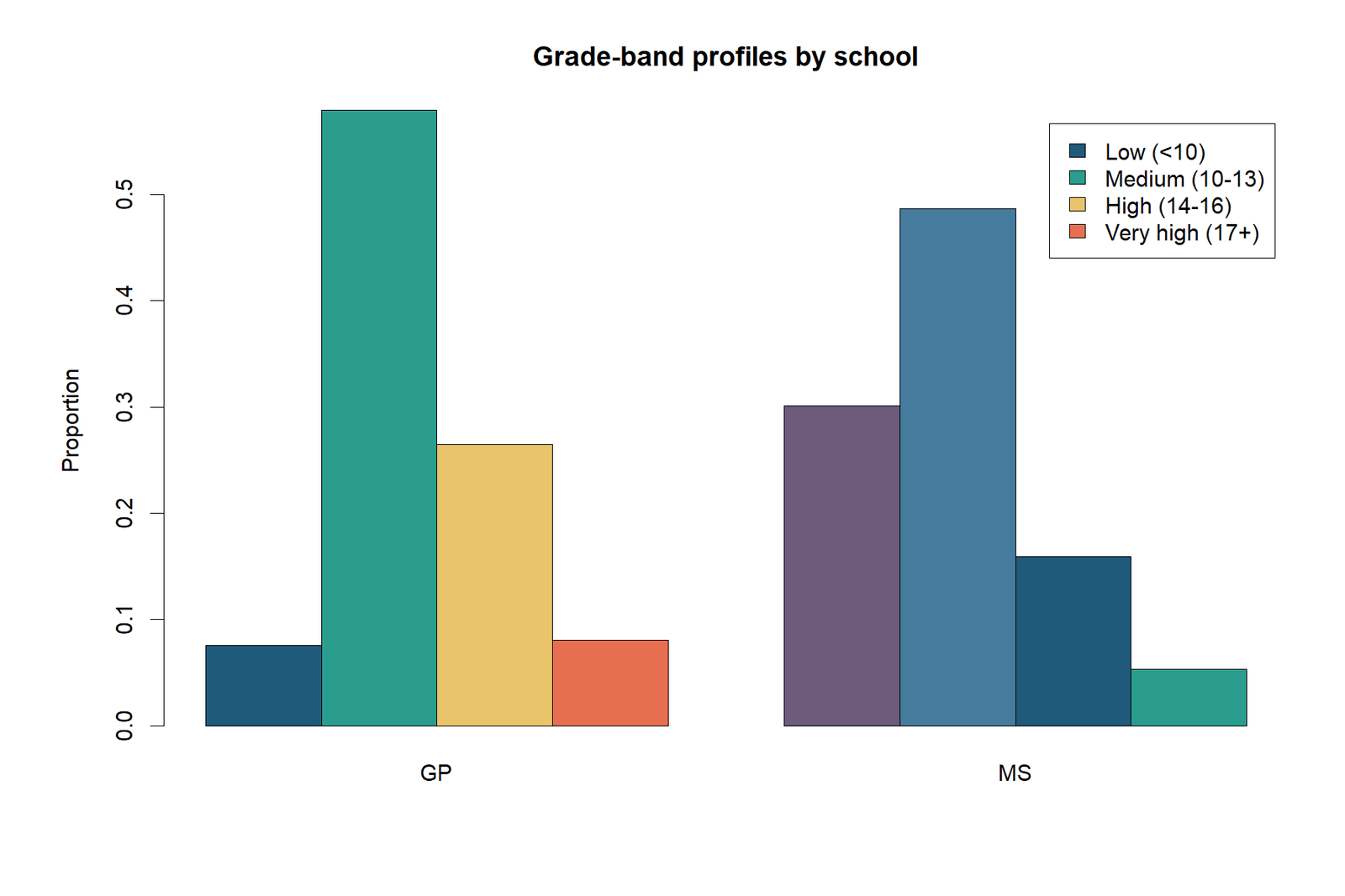
| GP | 7.565% | 57.920% | 26.478% | 8.038% |
| MS | 30.088% | 48.673% | 15.929% | 5.310% |
| MS − GP difference | +22.523 points | −9.247 points | −10.548 points | −2.728 points |
The dominant substantive contrast is the low grade band: 30.09% of MS students are in Low compared with 7.57% of GP students. GP has higher proportions in every band from Medium upward. The Fisher Freeman Halton Test evaluates the entire table simultaneously rather than choosing one cell after seeing the data.
Column composition
Among all Low-band students, 68% are from MS and 32% are from GP. By contrast, GP supplies 69.0% of Medium students, 75.7% of High students and 73.9% of Very-high students. These percentages are descriptive and should not be confused with within-school risks.
Expected Counts, Pearson Residuals and Cell Contributions
Expected counts are not used to compute the exact table probability, but they provide familiar descriptive context and identify where the association is concentrated.
| Cell | Observed | Expected | Pearson residual | χ² contribution |
|---|---|---|---|---|
| GP, Low | 32 | 65.1772 | −4.1095 | 16.8882 |
| GP, Medium | 245 | 231.3790 | +0.8955 | 0.8018 |
| GP, High | 112 | 96.4622 | +1.5820 | 2.5028 |
| GP, Very high | 34 | 29.9815 | +0.7339 | 0.5386 |
| MS, Low | 68 | 34.8228 | +5.6222 | 31.6094 |
| MS, Medium | 110 | 123.6210 | −1.2251 | 1.5008 |
| MS, High | 36 | 51.5378 | −2.1643 | 4.6844 |
| MS, Very high | 12 | 16.0185 | −1.0040 | 1.0081 |
The two Low-band cells contribute 48.4976 of the total Pearson χ² = 59.5340, or roughly 81.5% of the asymptotic statistic. This reveals that the school difference is primarily a low-band concentration, with a secondary deficit of MS students in the High band.
Residuals are descriptive diagnostics. The exact p-value is still based on conditional table probabilities, not on treating Pearson residuals as independent tests. For more context, see studentized residuals, Cramer's V and effect size.
Worked 2 × 4 Table and Complete Results
The Fisher Freeman Halton Test result should be read with the school profiles, residuals and Cramer's V rather than as a stand-alone threshold decision.
Probability of this one table given its margins.
50,000 fixed-margin resamples.
df = 3, p = 7.3925 × 10⁻¹³.
Moderate descriptive association.
No expected cells below 5.
At α = .05 and stricter levels.
Primary inference
The Fisher Freeman Halton Test indicates that school and final-grade band are not conditionally independent. The exact-reference Monte Carlo estimate is far below .05. The observed pattern is therefore too improbable to attribute to fixed-margin random allocation alone.
Effect-size interpretation
Cramer's V = 0.3029 is calculated from the Pearson statistic and is best described as a moderate descriptive association in this 2 × 4 table. The Fisher Freeman Halton Test itself does not automatically produce a unique confidence interval for Cramer's V. A bootstrap interval can be added as a separate analysis, but it should not be presented as part of the exact conditional test unless the method is stated.
Practical interpretation
MS has a much larger Low-band share and smaller Medium, High and Very-high shares than GP. The biggest absolute profile difference is 22.52 percentage points in the Low band. Because grade bands are ordered, an applied report can discuss the direction descriptively while noting that the exact test is a general association test rather than an ordinal trend test.
Fisher Freeman Halton Test Versus Related Tests
The Fisher Freeman Halton Test is selected from the table design and conditioning logic, not because its p-value is expected to be smaller than an asymptotic alternative.
Conditional exact test for a 2 × 2 table.
Conditional exact extension for larger r × c tables.
Asymptotic independence test using observed and expected counts.
Stratified or score-based association methods when structure is present.
| Method | Table/design | Conditioning | Worked result | Main role |
|---|---|---|---|---|
| Fisher Freeman Halton Test | 2 × 4 | All margins fixed | Monte Carlo p = .0000199996 | Primary exact-reference analysis. |
| Pearson chi-square | 2 × 4 | No exact conditioning | χ²(3) = 59.5340, p = 7.3925e−13 | Asymptotic comparison and residual context. |
| Likelihood-ratio chi-square | 2 × 4 | Asymptotic | G²(3) = 57.075, p < .001 | Alternative asymptotic statistic. |
| Cochran-Mantel-Haenszel score test | Ordered or stratified structure | Depends on formulation | Not the primary test here | Useful if ordinal trend or strata are the research focus. |
Fisher exact test versus Fisher Freeman Halton
The 2 × 2 Fisher exact test and the Fisher Freeman Halton Test use the same conditional principle. The distinction is table size. A 2 × 4 table cannot be reduced to a set of independent 2 × 2 tests without changing the global question and creating multiple-testing problems.
Fisher Freeman Halton versus chi-square
The Pearson result is even smaller numerically, but the methods answer the same null through different reference distributions. Because all expected counts exceed 5, the close qualitative agreement is unsurprising. Method selection should be based on design and inferential preference, not on which p-value is smaller.
Fisher Freeman Halton versus Barnard and Boschloo
Barnard's Exact Test and Boschloo Test are unconditional procedures for 2 × 2 comparisons. They do not directly replace the Fisher Freeman Halton Test for a 2 × 4 table.
Fisher Freeman Halton Test Calculator Workflow
A valid Fisher Freeman Halton Test calculator must disclose whether it uses complete enumeration, a network algorithm or fixed-margin Monte Carlo sampling.
A reliable Fisher Freeman Halton Test calculator must accept the full r × c count matrix, preserve the selected margins, define two-sided extremeness and disclose whether it enumerates every table or estimates the p-value by Monte Carlo.
Calculator inputs for the worked 2 × 4 table
| Input | GP | MS | Check |
|---|---|---|---|
| Low | 32 | 68 | Column total 100 |
| Medium | 245 | 110 | Column total 355 |
| High | 112 | 36 | Column total 148 |
| Very high | 34 | 12 | Column total 46 |
| Row totals | 423 | 226 | Grand total 649 |
Step-by-step calculator checks
- Enter counts, not percentages.
- Confirm the table orientation and all six margins.
- Select a two-sided probability-ordered test unless a prespecified alternative is available.
- Choose exact enumeration or a sufficiently large Monte Carlo B.
- Set and record a random seed for reproducibility.
- Verify that the observed table probability is about 4.8604 × 10⁻¹⁶.
- Verify that the 50,000-resample add-one p-value is 1/50,001.
- Report row profiles and a descriptive association measure beside the p-value.
What a calculator should not claim
A calculator should not label the observed table mass as the p-value, return p = 0, silently switch to Pearson chi-square, or present a confidence interval for the test itself without identifying a separate effect-size or model-based procedure.
Python and R Fisher Freeman Halton Test Chart Interpretations
Each Fisher Freeman Halton Test chart below is tied to the verified table, margins, simulation settings and exact numerical interpretation.
The Python report presents six chart stories with exact values and next-step guidance. The R report presents six complementary figures in three paired rows so observed tables, expected tables, residuals, row profiles, probability scales and the final result can be compared directly.
Python Fisher Freeman Halton Test Charts
The Python charts move from the observed table to expected counts, residual diagnostics, Monte Carlo resolution and a compact result summary. Each chart is interpreted with exact values rather than generic visual commentary.
Chart 1: Observed 2 × 4 tablePython
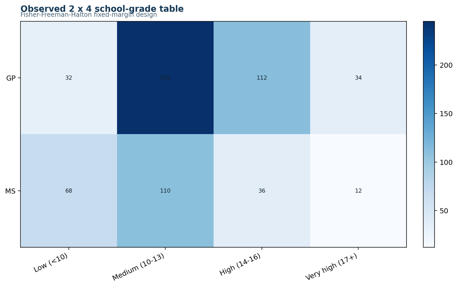
GP is concentrated in Medium and High, while MS has a much larger Low-band cell.
GP counts are 32, 245, 112 and 34; MS counts are 68, 110, 36 and 12.
The largest contrast is not a simple sample-size effect. MS has fewer total students but more Low-band students.
The fixed-margin exact analysis evaluates the entire eight-cell pattern while retaining all row and column totals.
Chart 2: Fixed-margin expected countsPython
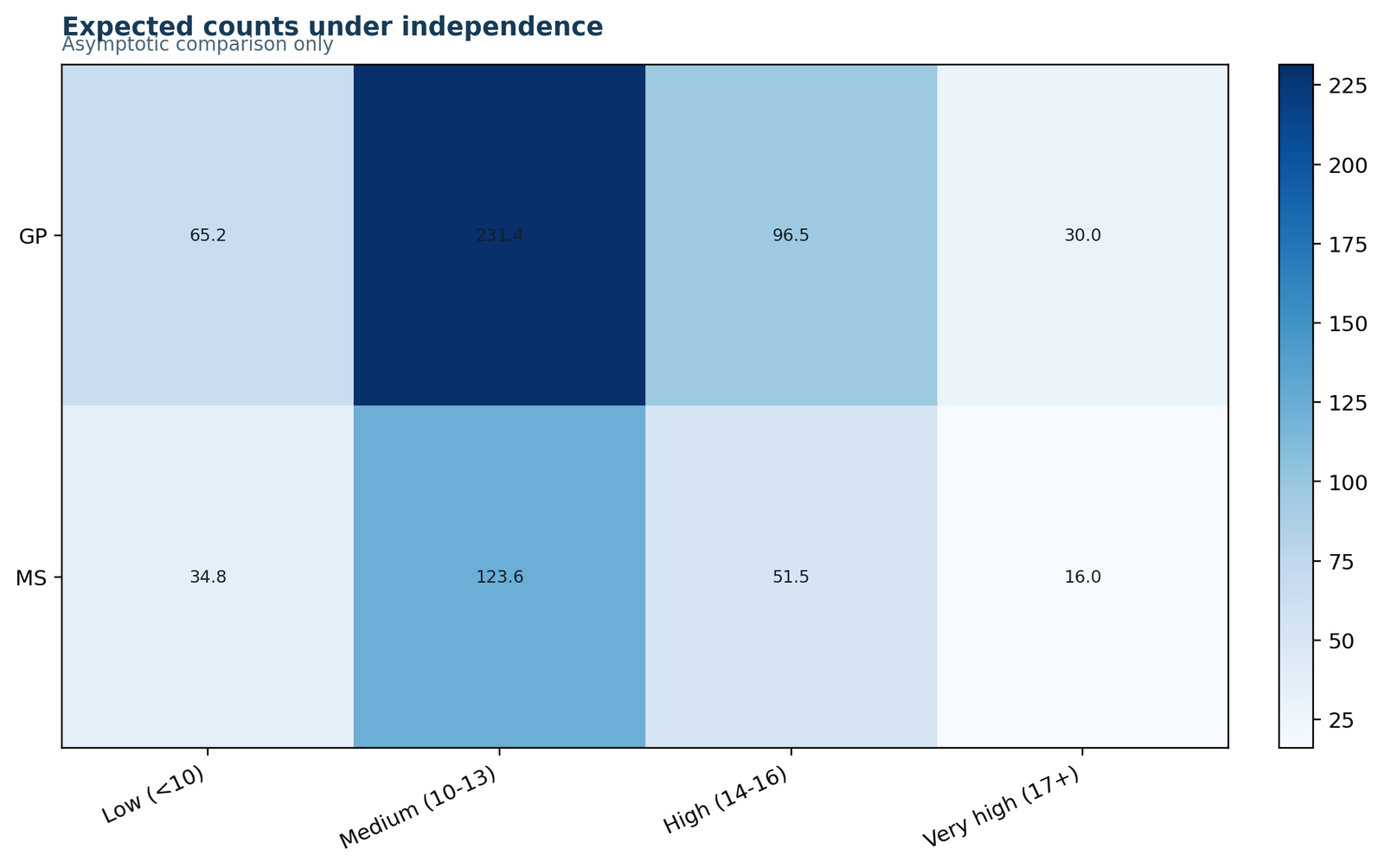
The expected Low counts are reversed relative to the observed pattern: GP would be expected to have about 65.18 and MS about 34.82.
Expected GP counts are 65.177, 231.379, 96.462 and 29.982; MS counts are 34.823, 123.621, 51.538 and 16.018.
All expected cells exceed 16, so the Pearson approximation is not threatened by small expected counts in this example.
The exact test remains valid; expected counts are included to explain where the association arises.
Chart 3: Pearson residual patternPython
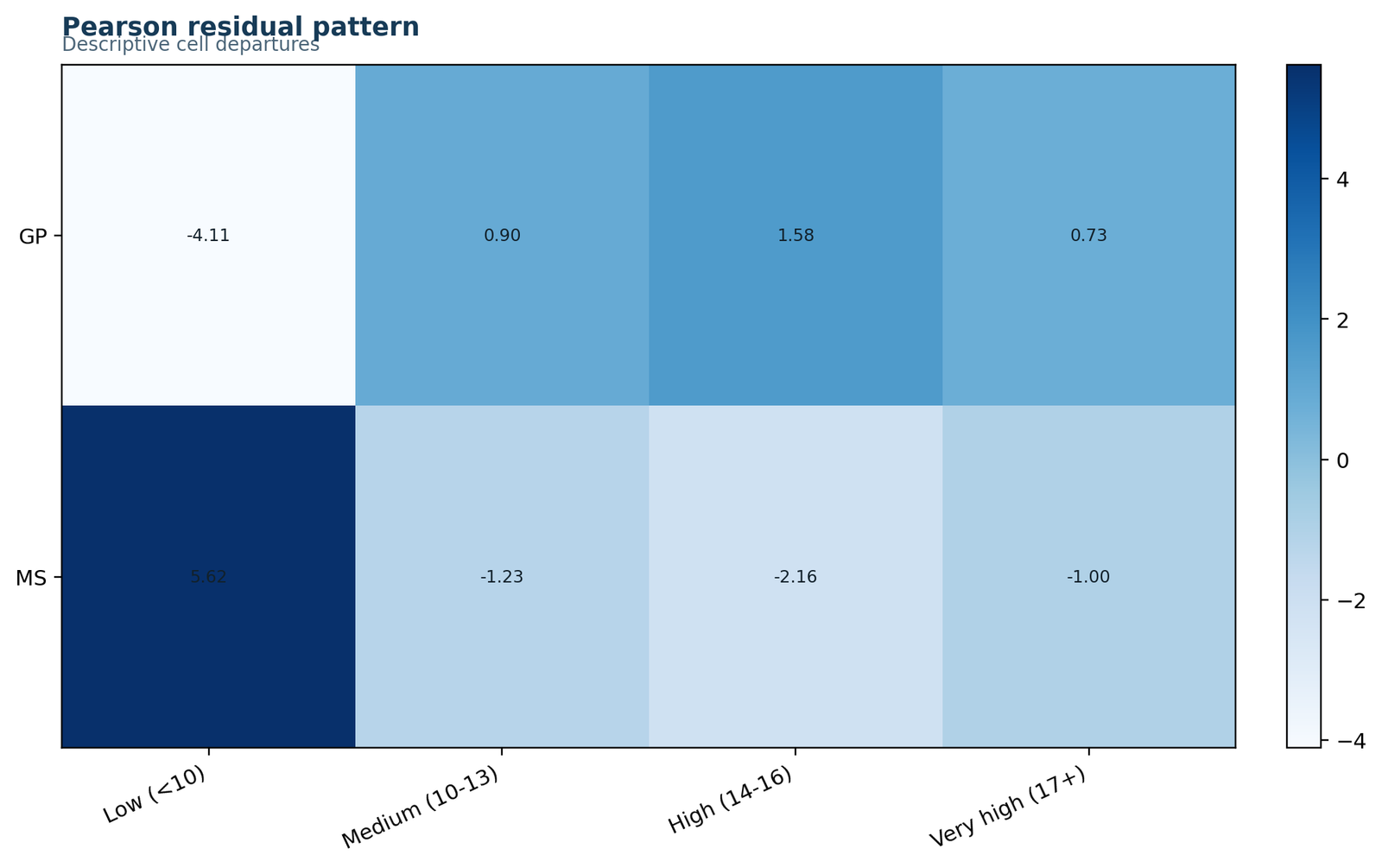
The most extreme positive residual is MS-Low, and the most extreme negative residual is GP-Low.
Residuals are GP: −4.110, 0.895, 1.582, 0.734; MS: 5.622, −1.225, −2.164, −1.004.
MS has far more Low cases than independence predicts, while GP has far fewer. MS also has a notable High-band deficit.
Residuals identify the cells responsible for the association but do not replace the global exact p-value.
Chart 4: Monte Carlo exact p-value convergencePython
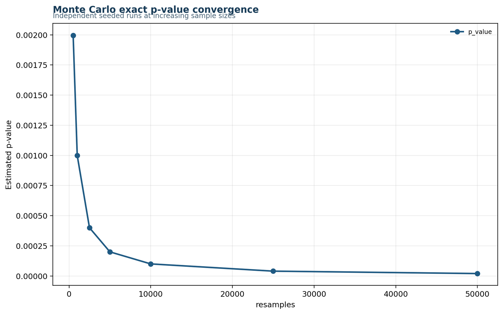
The plotted estimate decreases almost exactly as 1/(B+1).
Values are .001996 at B=500, .000999 at 1,000, .00039984 at 2,500, .00019996 at 5,000, .00009999 at 10,000, .0000399984 at 25,000 and .0000199996 at 50,000.
The sequence indicates zero sampled tables meeting the probability-ordering extremeness rule at each run size.
The chart documents a resolution floor, not proof that the unknown p-value equals the final decimal exactly.
Chart 5: Monte Carlo precisionPython
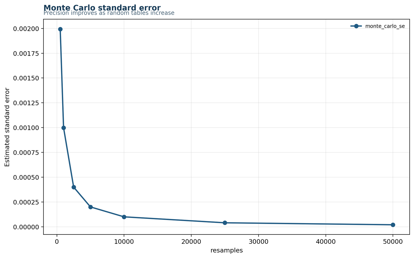
The displayed uncertainty decreases with B and reaches roughly 2 × 10⁻⁵ at 50,000 samples.
The final displayed Monte Carlo standard-error quantity is approximately 1.99994 × 10⁻⁵.
When no extreme tables are observed, ordinary plug-in precision formulas require cautious interpretation because the estimate sits at the add-one boundary.
The visual appropriately warns readers not to treat a random Monte Carlo result as infinitely precise.
Chart 6: Exact and asymptotic result summaryPython
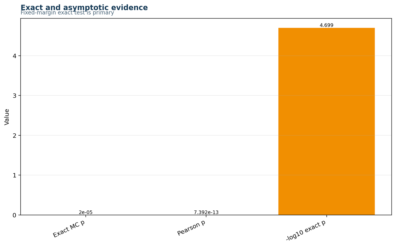
Both the exact-reference estimate and Pearson p-value indicate strong evidence against independence.
Monte Carlo p = 2.0 × 10⁻⁵; Pearson p = 7.392 × 10⁻¹³; −log10 of the exact estimate is about 4.699.
The two methods differ numerically because they use different reference distributions and because the Monte Carlo p-value is resolution-limited.
The decision is stable across exact and asymptotic approaches, strengthening the substantive conclusion.
R Fisher Freeman Halton Test Charts in Paired Rows
The R report reproduces the table, expected counts, residuals, row profiles and exact-probability concepts. The six R charts are arranged in three responsive pairs, with one explanation card aligned to each chart.
R pair 1: Observed and expected 2 × 4 tables
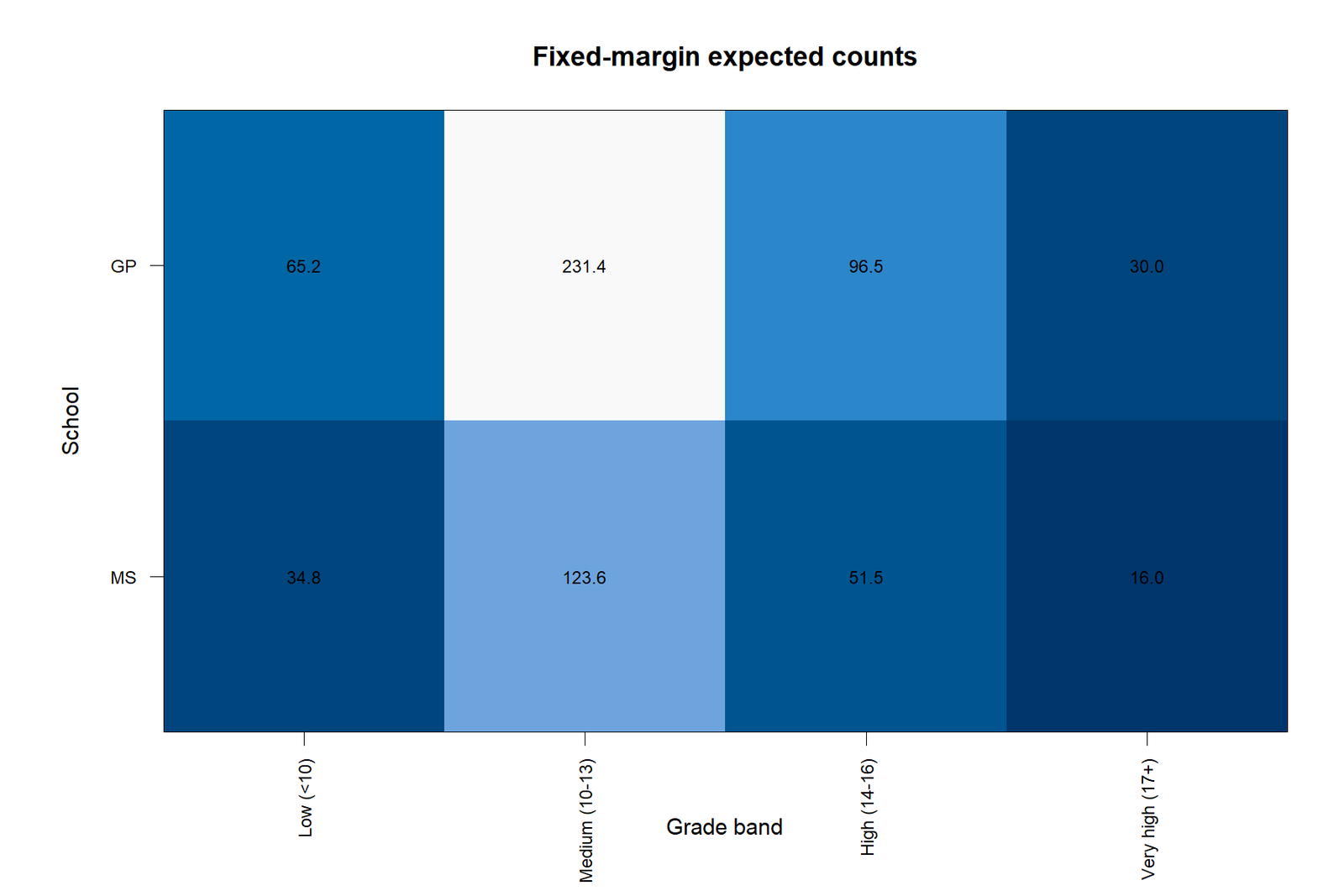
Observed allocation differs sharply in the Low band
The observed R table confirms 32 GP-Low cases and 68 MS-Low cases, despite GP having the larger total sample. Medium and High counts are concentrated in GP.
Expected counts provide the null benchmark
Under independence, Low counts would be 65.18 for GP and 34.82 for MS. The observed allocation is nearly reversed, creating the dominant departure.
R pair 2: Pearson residuals and row profiles
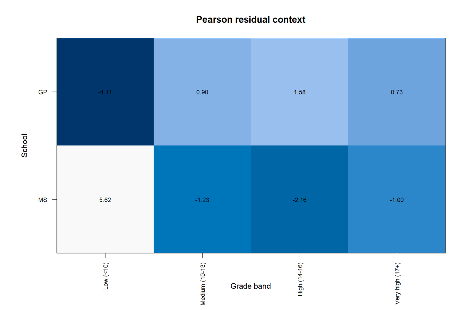
Residuals isolate the strongest cells
MS-Low has residual +5.62 and GP-Low has −4.11. MS-High is also lower than expected with residual −2.16.
Profiles translate counts into practical percentages
Low is 7.57% in GP and 30.09% in MS. GP exceeds MS in Medium, High and Very high bands.
R pair 3: Exact probability scales and result summary
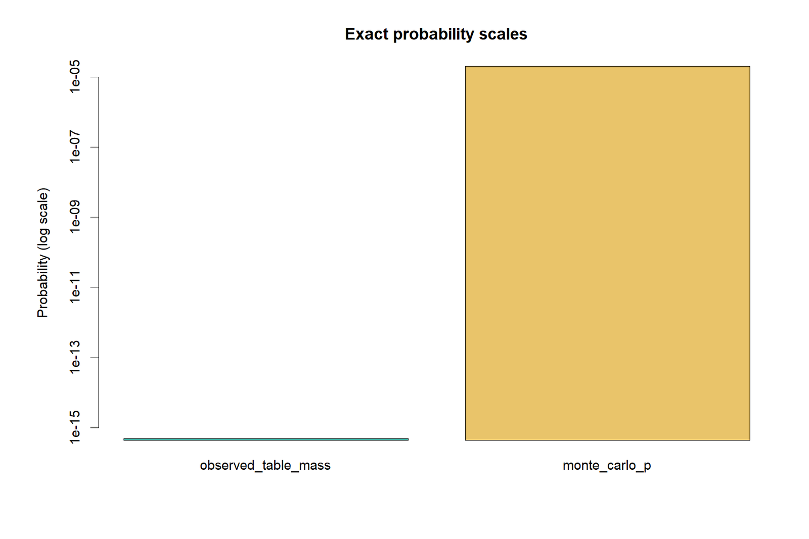
Table mass and p-value are fundamentally different
The observed table mass is 4.86 × 10⁻¹⁶, whereas the two-sided Monte Carlo p-value is 2.0 × 10⁻⁵. The p-value is larger because it aggregates the probabilities of many extreme tables.
Primary and supporting tests agree on rejection
The exact-reference analysis is primary; Pearson χ² = 59.534 provides supporting asymptotic context. Both show that school and grade band are associated.
Fisher Freeman Halton Test in Python, R, SPSS, SAS, Stata and Excel
A reproducible Fisher Freeman Halton Test workflow should return the same observed table, reference margins and inferential conclusion across software environments.
Fisher Freeman Halton Test in Python
A modern Python workflow can represent the null with fixed-margin random tables, compute the multivariate-hypergeometric mass, and estimate the two-sided probability-ordered p-value. See categorical data analysis in Python.
- Store the table as a 2 × 4 integer array.
- Compute margins and log-factorial table mass.
- Sample random tables with exactly those margins.
- Count tables whose mass is no greater than the observed mass.
- Use add-one correction and a fixed seed.
- Export counts, expected values, residuals and simulation diagnostics.
Fisher Freeman Halton Test in R
R's fisher.test handles larger contingency tables and can use simulated p-values when direct exact computation is impractical. See categorical data analysis in R.
- Create the 2 × 4 matrix with correct row and column labels.
- Set a seed before simulation.
- Use
simulate.p.value=TRUEand a declared B. - Check that all margins match the workbook.
- Report the simulation setting with the p-value.
Fisher Freeman Halton Exact Test in SPSS
SPSS Exact Tests extends Fisher's test to larger r × c tables when the Exact Tests functionality is available. The supplied SPSS output also provides counts, expected counts, row percentages, residuals, Pearson χ² and Cramer's V. See categorical data analysis in SPSS.
- Use CROSSTABS for the school-by-band table.
- Request counts, row percentages, expected counts and residuals.
- Select Exact or Monte Carlo in the exact-tests dialog.
- Record confidence level, sample count and seed settings.
- Do not relabel the asymptotic Pearson p-value as the exact result.
Fisher Freeman Halton Test in Excel
The worked Excel workbook reproduces the observed table mass exactly using log-factorials. Excel is suitable for transparent calculation of one table's conditional mass, margins, expected counts and Pearson context. Complete exact enumeration or fixed-margin random-table simulation requires VBA, Office Scripts or an external validated engine.
- Use
COUNTIFSto construct the observed table. - Use
GAMMALN(n+1)for log-factorials. - Exponentiate the final log mass.
- Store verified Monte Carlo results with B and seed.
- Do not use
FISHERworksheet functions; they refer to Fisher transformations, not Fisher's exact test.
Fisher Freeman Halton Test in SAS
SAS exact-test facilities can request exact contingency-table inference in PROC FREQ, subject to available options and computational limits. Use weighted count data or row-level records, request exact tests, and save ODS output for reproducibility.
Fisher Freeman Halton Test in Stata
Stata workflows may use exact or user-contributed routines for r × c tables, depending on version and table size. Confirm whether the command uses complete enumeration, network algorithms or Monte Carlo, and report the settings rather than assuming every “exact” label has identical implementation.
Expandable Fisher Freeman Halton Test Code
Python fixed-margin Monte Carlo outline
import numpy as np
from math import lgamma, exp
from scipy.stats import random_table

observed = np.array([[32, 245, 112, 34],
                     [68, 110,  36, 12]], dtype=int)
row = observed.sum(axis=1)
col = observed.sum(axis=0)
N = observed.sum()

def log_mass(table):
    return (sum(lgamma(x + 1) for x in row)
            + sum(lgamma(x + 1) for x in col)
            - lgamma(N + 1)
            - sum(lgamma(x + 1) for x in table.ravel()))

obs_log_mass = log_mass(observed)
rng = np.random.default_rng(20260716)
B = 50000
extreme = 0
for table in random_table.rvs(row, col, size=B, random_state=rng):
    if log_mass(table) <= obs_log_mass + 1e-12:
        extreme += 1
p_mc = (extreme + 1) / (B + 1)
R simulated fixed-margin test
tab <- matrix(c(32,245,112,34,
                68,110,36,12),
              nrow=2, byrow=TRUE)
rownames(tab) <- c("GP","MS")
colnames(tab) <- c("Low","Medium","High","Very high")
set.seed(20260716)
fisher.test(tab, simulate.p.value=TRUE, B=50000)
SPSS crosstab and exact-test outline
CROSSTABS
 /TABLES=school_n BY grade3
 /FORMAT=AVALUE TABLES
 /STATISTICS=CHISQ PHI
 /CELLS=COUNT ROW COLUMN EXPECTED RESID
 /COUNT ROUND CELL.

* In the Exact Tests dialog, request the Fisher-Freeman-Halton exact
* or Monte Carlo result and record the sampling settings.
Excel observed-table probability formula logic
Log numerator = GAMMALN(row1+1)+GAMMALN(row2+1)
              + SUM(GAMMALN(each column total+1))
Log denominator = GAMMALN(N+1)
                + SUM(GAMMALN(each observed cell+1))
Observed table mass = EXP(Log numerator - Log denominator)
Assumptions, Limitations and Interpretation Safeguards
The Fisher Freeman Halton Test remains valid only when independent cases, mutually exclusive categories and the declared fixed-margin reference model match the study design.
Core conditions
- Each observation contributes to one table cell.
- Cases are independent of one another.
- Categories are mutually exclusive.
- The fixed-margin conditioning scheme is scientifically acceptable.
- Monte Carlo samples are generated from the correct conditional distribution.
- Simulation settings are sufficient for the desired precision.
Common mistakes
- Calling the observed table mass the p-value.
- Reporting Monte Carlo p = 0.
- Hiding the number of resamples or seed.
- Using percentages instead of integer counts as input.
- Interpreting nominal exact association as an ordinal trend.
- Running many 2 × 2 Fisher tests instead of one global r × c test.
Independence of cases
The {P} does not correct repeated observations, clusters, siblings, classrooms or paired measurements. If students are clustered within classes or schools beyond the row grouping, a multilevel or generalized estimating approach may be necessary. See generalized estimating equations and multilevel regression.
Fixed margins are a modeling choice
Conditional inference treats both row and column totals as fixed for the reference distribution. This is mathematically well-defined, but analysts should still explain why that conditioning is reasonable for the study design. An exact method is not automatically the best method for every data-generating process.
Effect size and confidence interval
The {P} is a significance test. It does not supply one universally accepted effect-size confidence interval. Report the observed row profiles and Cramer's V, and add bootstrap or model-based intervals only when the method is clearly named. See confidence interval and margin of error.
APA Reporting for the Fisher Freeman Halton Test
In formal writing, name the Fisher Freeman Halton Test explicitly and report the Monte Carlo implementation rather than using the vague label “an exact test.”
An APA-style report should identify the table, fixed-margin conditional method, two-sided ordering rule, Monte Carlo sample count, random seed, estimated p-value, descriptive profiles and a suitable association measure. The observed table probability should never be mislabeled as the test p-value.
What to Include in an APA-Style Report
Method Information
- Fisher Freeman Halton Test
- 2 × 4 contingency table
- Probability-ordered, fixed-margin reference distribution
- 50,000 Monte Carlo tables
- Seed = 20260716
Results Information
- Monte Carlo p = 1/50,001 = .000020
- Observed table mass = 4.8604 × 10⁻¹⁶
- Pearson χ²(3, N = 649) = 59.53
- Cramer's V = .303
- GP and MS grade-band profiles
APA-Style Methods Sentence
A Fisher Freeman Halton Test was used to evaluate the association between school and four G3 grade bands in a 2 × 4 contingency table. The analysis conditioned on the observed row and column margins and estimated a two-sided probability-ordered p-value from 50,000 fixed-margin Monte Carlo tables using seed 20260716.
Full APA-Style Results Example
The distribution of G3 grade bands differed by school according to a Fisher Freeman Halton Test with 50,000 fixed-margin Monte Carlo samples, p = 1/50,001 = .000020. The strongest profile difference occurred in the Low band, which contained 7.57% of GP students and 30.09% of MS students. Pearson's comparison also rejected independence, χ²(3, N = 649) = 59.53, p < .001, Cramer's V = .303.
Reusable APA Templates for the Fisher Freeman Halton Test
Significant fixed-margin result
Reject H₀
A Fisher Freeman Halton Test evaluated the association between row variable and column variable in a r × c table.
The two-sided probability-ordered p-value used B fixed-margin Monte Carlo tables with seed seed.
The variables were associated, p = Monte Carlo p, with Cramer's V = effect size.
Use this template when the global exact-reference result is statistically significant.
Non-significant fixed-margin result
Retain H₀
A Fisher Freeman Halton Test compared row categories across column categories.
The fixed-margin evidence did not indicate an association, p = p-value.
Observed profiles and Cramer's V = effect size were reported to describe uncertainty and magnitude.
Do not describe a non-significant result as proof that the distributions are identical.
Monte Carlo floor or zero exceedances
Resolution note
No sampled table among B fixed-margin replicates was at least as improbable as the observed table.
Using the add-one correction, the estimate was p = 1/(B + 1) = p-value.
The result was at the simulation resolution floor and should not be reported as p = 0 or as a fully enumerated exact decimal.
This is the correct template for the present 50,000-table analysis.
APA-Style Table Note
APA Rounding Rules
- Report the Monte Carlo result as p = .000020 or p < .001 in prose, while retaining 1/50,001 in technical documentation.
- Report χ² = 59.53 and Cramer's V = .303.
- Give percentages to one or two decimal places and raw counts in the same table or sentence.
- Never report the simulation result as p = 0.
Common Fisher Freeman Halton Test Mistakes and How to Correct Them
| Mistake | Why it is wrong | Correction |
|---|---|---|
| Calling the observed table probability the p-value | The single-table mass covers only one table, while the two-sided p-value sums all qualifying tables. | Report 4.8604 × 10⁻¹⁶ as the observed table probability and .000020 as the Monte Carlo p-value. |
| Reporting p = 0 after zero simulated exceedances | A finite simulation cannot establish a literal zero probability. | Use the add-one estimate (b + 1)/(B + 1) and state the simulation resolution. |
| Ignoring the fixed-margin design | The conditional reference set depends on which margins are held fixed. | State the row totals, column totals and conditional sampling rule. |
| Replacing a global 2 × 4 test with many 2 × 2 tests | Pairwise tests change the research question and inflate multiplicity. | Use one global Fisher Freeman Halton Test, then prespecified follow-up analyses if needed. |
| Treating ordered categories as if the test estimates trend | The general test treats categories nominally. | Add an ordinal score or regression analysis when monotonic trend is the scientific target. |
| Reporting significance without profiles or effect size | A tiny p-value does not describe how the distributions differ or how large the association is. | Report row percentages, key residuals and Cramer's V. |
Reports and Worked Excel Download
Frequently Asked Questions
What is the Fisher Freeman Halton Test?
The Fisher Freeman Halton Test is the conditional exact extension of Fisher's exact test to contingency tables larger than 2 × 2. It tests row-column independence while conditioning on observed margins.
When should I use the Fisher Freeman Halton Test?
Use it for an r × c table with independent observations when exact conditional inference is desired, especially when expected counts are sparse or unbalanced.
Is the Fisher Freeman Halton Test only for 2 × 3 tables?
No. It applies generally to r × c contingency tables, subject to computational feasibility and software implementation.
Is the observed table probability the p-value?
No. The observed table probability is one probability mass. The two-sided p-value aggregates the masses of all tables meeting the extremeness definition.
Why is the Monte Carlo p-value 1/50,001?
No sampled table among 50,000 replicates was at least as improbable as the observed table. With add-one correction, the estimate is (0+1)/(50,000+1).
Can the Fisher Freeman Halton Test return p = 0?
A Monte Carlo report should not return p = 0. Use an add-one estimate or state a resolution-aware bound. Complete exact enumeration can produce a very small positive value, not literal zero.
What effect size accompanies the Fisher Freeman Halton Test?
Cramer's V is commonly reported as descriptive association strength. It comes from the Pearson statistic and is not itself an exact-test statistic.
Does the Fisher Freeman Halton Test use category order?
No. The general test treats categories nominally. Use an ordinal method when a monotonic trend or ordered effect is the scientific target.
How do I run the Fisher Freeman Halton Test in R?
Construct the r × c table and use fisher.test. For large tables, set a seed and request a simulated p-value with a sufficiently large number of replicates.
How do I run the Fisher Freeman Halton Exact Test in SPSS?
Build the crosstab, open Exact Tests, and request the exact or Monte Carlo extension. Availability depends on the SPSS exact-testing functionality and version.
Can Excel calculate the Fisher Freeman Halton Test?
Excel can calculate the probability mass of the observed table with log-factorials. The full p-value needs enumeration or fixed-margin simulation, normally through VBA, Office Scripts or validated external software.
What is the worked conclusion?
The school and grade-band distributions differ strongly. The fixed-margin Monte Carlo estimate is .0000199996, and the largest difference is the much higher Low-band proportion in MS.
Fisher Freeman Halton Test Conclusion
The Fisher Freeman Halton Test provides the global fixed-margin conclusion, while row profiles and residuals explain the practical pattern behind that conclusion.
The {P} provides exact conditional logic for contingency tables larger than 2 × 2. In the verified 2 × 4 school-by-grade-band example, the observed table mass was 4.8604 × 10⁻¹⁶, and no table among 50,000 fixed-margin Monte Carlo replicates was at least as improbable as the observed table. The add-one estimate was therefore 1/50,001 = 0.0000199996, providing strong evidence against conditional independence.
The statistical conclusion is reinforced by Pearson χ²(3) = 59.5340 and Cramer's V = 0.3029. The substantive pattern is concentrated in the Low grade band: MS has a 30.09% Low-band rate compared with 7.57% for GP. A complete report should combine the {P}, simulation settings, observed row profiles, effect-size context and a clear distinction between observed table mass and the two-sided p-value.
Continue with Chi Square Test of Independence, Cramer's V, Cochran Mantel Haenszel Test and Categorical Data Analysis in R for related categorical-analysis workflows.

