
Regression Confidence Interval: Formula, Interpretation, Python, R, SPSS and Excel Guide
Regression Confidence Interval analysis explains how uncertainty changes when the target is a regression coefficient, the conditional mean at a predictor profile, or one future individual’s outcome. This worked guide uses 649 complete cases, six predictors, exact 90%, 95% and 99% coefficient limits, eight Python charts and four R validation charts.
6 predictors
95% t critical = 1.9637
Prediction width = 4.9529
Regression Confidence Interval Model Overview
Regression Confidence Interval is not one single interval. In regression, uncertainty can be attached to a coefficient, an estimated mean response, or an individual prediction. These three targets have different interpretations and different formulas even when they come from the same fitted equation.
The worked model predicts G3 from G1, G2, studytime, failures, absences and age. It contains 649 complete cases, six slopes and an intercept. The fitted equation has R² = 0.8506, adjusted R² = 0.8492 and residual standard error = 1.2544.
What Is a Regression Confidence Interval?
A Regression Confidence Interval is a range generated from a fitted model and a standard-error formula. The target determines what the interval means. Readers must therefore identify the estimand before reading the endpoints.
For basic background, read Confidence Interval, Standard Error and Margin of Error.
Research Question Answered by Each Interval
A coefficient interval asks: what population slope values are reasonably compatible with this sample? A fitted-mean interval asks: what is the plausible average outcome for all cases sharing this predictor profile? An individual prediction interval asks: what outcome range is plausible for one new case with that profile?
These questions are related but not interchangeable. The mean interval can be very narrow while the individual prediction interval remains wide because real people vary around the mean.
When Should Regression Confidence Interval Analysis Be Used?
Appropriate uses
- Reporting uncertainty around regression coefficients.
- Estimating an average response at a chosen predictor profile.
- Forecasting one future outcome with an individual prediction interval.
- Comparing precision at 90%, 95% and 99% confidence levels.
- Evaluating how leverage changes mean-response uncertainty.
Common misuses
- Using a coefficient interval as a range for an outcome.
- Using a mean confidence band for an individual forecast.
- Interpreting 95% as a posterior probability for the coefficient.
- Ignoring heteroskedasticity, dependence or model misspecification.
- Comparing intervals produced from different rows or model formulas.
Regression Confidence Interval Formula for a Coefficient
Every coefficient uses the same confidence level and residual degrees of freedom, but each term has its own standard error. At the 95% level with 642 residual degrees of freedom, the critical value is 1.963665968734212.
Regression Confidence Interval Formula for the Mean Response
The fitted-mean standard error depends on where the predictor profile sits within the design. Profiles near the center of the observed predictor space generally have narrower intervals, while high-leverage profiles have wider intervals.
Individual Prediction Interval Formula
The additional 1 inside the square root represents new individual residual variation. It is the main reason individual limits are much wider than mean-response limits.
How Confidence Level Changes Width
Increasing the confidence level from 90% to 95% or 99% increases the critical value. The coefficient estimate and standard error remain unchanged, but the margin of error becomes larger.
In this model, the failures interval excludes zero at 95% but includes zero at 99%. This does not mean the coefficient changed; the demanded coverage became more conservative.
Relation to P-Values
Under the same classical assumptions, a two-sided 95% coefficient interval excludes zero exactly when the corresponding p-value is below .05. The interval is more informative because it also shows direction, plausible magnitude and precision.
Use P-Value and Null and Alternative Hypothesis for the testing framework.
Core Assumptions
1. Correct mean function
The regression equation must represent the conditional mean adequately. Omitted curvature or interactions can bias estimates and intervals.
2. Independent observations
Residual dependence can make classical standard errors too small. Clustered, repeated or time-ordered data need suitable corrections.
3. Appropriate variance treatment
Classical intervals assume constant residual variance. Robust standard errors may be needed when variance changes, but individual prediction limits require additional care.
4. Credible residual distribution
Exact small-sample t procedures rely on normal errors. With 649 cases, coefficient inference is often reasonably robust, but tail observations still matter.
5. Consistent coding and cases
Python, R, SPSS and Excel must use the same complete cases, formula, reference coding and confidence level.
6. No unsupported extrapolation
Intervals outside the observed predictor region can be misleading even when the calculations are arithmetically correct.
Advantages
- Shows direction and precision rather than only statistical significance.
- Separates average-response uncertainty from individual prediction uncertainty.
- Allows direct arithmetic cross-checks through midpoint and width.
- Supports transparent comparison across confidence levels and software.
Limitations
- Intervals inherit every limitation of the fitted regression model.
- Classical intervals can be misleading under heteroskedasticity or dependence.
- In-sample inclusion is not external coverage validation.
- Linear prediction limits can extend beyond a bounded outcome scale.
Current Worked Scenario
The model uses 649 complete observations and predicts G3 from G1, G2, studytime, failures, absences and age. It has F(6,642) = 609.3527, p < .001, R² = 0.8506, adjusted R² = 0.8492, AIC = 2142.9548 and BIC = 2174.2828.
The average fitted-mean interval is 0.4806 grade points wide, while the average individual prediction interval is 4.9529 grade points wide. This tenfold difference is the main educational result of the analysis.
Quick Answer
Coefficient confidence intervals
- G1 and G2 are positive.
- Failures is negative.
- Absences is small and positive.
- Studytime and age cross zero.
Mean versus individual uncertainty
- Mean-response intervals are narrow.
- Individual prediction intervals are much wider.
- Mean-band observed inclusion is not individual coverage.
- Prediction inclusion is 97.23% in the fitted rows.
Table of Contents
- Why this analysis needs Regression Confidence Interval
- How the three interval types work
- Variables used and coding
- Exact results
- Eight Python chart stories
- R chart pairs and explanations
- Coefficient interpretation
- Mean and individual prediction meaning
- Assumptions and diagnostics
- Python, R, SPSS and Excel workflows
- Code
- Advanced topics
- APA-style reporting
- Publication checklist
- Downloads
- Related guides
- Frequently asked questions
Why This Analysis Needs Regression Confidence Interval
A point estimate such as G2 = 0.8834 does not reveal how precisely the population slope is estimated. A fitted value such as 13.32 does not reveal how uncertain the conditional mean is. A prediction for one student also needs residual variation that is absent from a mean-response interval.
Regression Confidence Interval analysis solves these three uncertainty problems separately. This separation is essential for honest reporting and practical decision-making.
The model is an Ordinary Least Squares Regression equation. Readers new to regression should first review Correlation vs Regression and Pearson Correlation.
How Regression Confidence Interval Works
Estimate coefficients and residual variance.
Coefficient, mean or individual.
Construct and verify the bounds.
Coefficient Example
Mean-Response Example
For source case 1, the fitted mean is 9.8775 and the mean interval is [9.0858, 10.6692]. The midpoint is 9.8775 and the width is 1.5835.
Individual Prediction Example
For the same predictor profile, the individual interval is [7.2901, 12.4648], with width 5.1747. The center is identical, but the prediction interval adds individual residual variation.
Variables Used, Coding and Interval Targets
| Variable / target | Role | Definition | Use in analysis |
|---|---|---|---|
| G3 | Outcome | Final student grade. | Continuous dependent variable |
| G1 | Predictor | First-period grade. | Continuous slope with coefficient interval |
| G2 | Predictor | Second-period grade. | Continuous slope with coefficient interval |
| studytime | Predictor | Weekly study-time category. | Ordinal numeric predictor |
| failures | Predictor | Number of previous class failures. | Count / ordinal predictor |
| absences | Predictor | Number of school absences. | Count predictor |
| age | Predictor | Student age in years. | Continuous predictor |
| Predicted mean | Interval target | Estimated average G3 for one predictor profile. | Mean-response confidence interval |
| Future individual G3 | Interval target | One new outcome at the same predictor profile. | Individual prediction interval |
Regression Confidence Interval Results
Same rows across outputs
G1, G2, studytime, failures, absences, age
df = 6, 642
Main prediction-width component
Model information criterion
Stronger complexity penalty
Exact 95% Coefficient Intervals
| Term | B | SE | t | p | 95% CI | Decision |
|---|---|---|---|---|---|---|
| Intercept | -0.5453 | 0.7626 | -0.7150 | .4748 | [-2.0429, 0.9522] | Crosses zero |
| G1 | 0.1422 | 0.0366 | 3.8856 | .0001 | [0.0703, 0.2140] | Positive interval |
| G2 | 0.8834 | 0.0342 | 25.8229 | <.001 | [0.8162, 0.9506] | Strong positive interval |
| studytime | 0.0946 | 0.0620 | 1.5263 | .1274 | [-0.0271, 0.2163] | Crosses zero |
| failures | -0.2332 | 0.0949 | -2.4560 | .0143 | [-0.4196, -0.0467] | Negative interval |
| absences | 0.0227 | 0.0109 | 2.0857 | .0374 | [0.0013, 0.0440] | Small positive interval |
| age | 0.0236 | 0.0435 | 0.5438 | .5868 | [-0.0617, 0.1090] | Crosses zero |
Exact Interval Changes across Confidence Levels
| Level | Term | Interval | Width | Zero decision |
|---|---|---|---|---|
| 90% | G1 | [0.0819, 0.2024] | 0.1205 | Excludes zero |
| 95% | G1 | [0.0703, 0.2140] | 0.1437 | Excludes zero |
| 99% | G1 | [0.0476, 0.2367] | 0.1891 | Excludes zero |
| 90% | G2 | [0.8270, 0.9398] | 0.1127 | Excludes zero |
| 95% | G2 | [0.8162, 0.9506] | 0.1344 | Excludes zero |
| 99% | G2 | [0.7950, 0.9718] | 0.1768 | Excludes zero |
| 90% | studytime | [-0.0075, 0.1967] | 0.2041 | Includes zero |
| 95% | studytime | [-0.0271, 0.2163] | 0.2434 | Includes zero |
| 99% | studytime | [-0.0655, 0.2547] | 0.3202 | Includes zero |
| 90% | failures | [-0.3895, -0.0768] | 0.3127 | Excludes zero |
| 95% | failures | [-0.4196, -0.0467] | 0.3728 | Excludes zero |
| 99% | failures | [-0.4784, 0.0121] | 0.4905 | Includes zero |
| 90% | absences | [0.0048, 0.0406] | 0.0358 | Excludes zero |
| 95% | absences | [0.0013, 0.0440] | 0.0427 | Excludes zero |
| 99% | absences | [-0.0054, 0.0508] | 0.0562 | Includes zero |
| 90% | age | [-0.0480, 0.0953] | 0.1432 | Includes zero |
| 95% | age | [-0.0617, 0.1090] | 0.1707 | Includes zero |
| 99% | age | [-0.0887, 0.1360] | 0.2246 | Includes zero |
Mean-response summary
- Average width = 0.4805828761
- Median width = 0.4371368259
- Observed individual inclusion = 14.6379%
- Width changes with leverage
Individual prediction summary
- Average width = 4.9529178178
- Median width = 4.9458365569
- Observed inclusion = 97.2265%
- Residual variance dominates width
Download the Regression Confidence Interval Reports
The same verified output links appear again in the Downloads section.
Eight Python Chart Stories
Each figure uses the saved four-box explanation pattern: what the chart shows, exact values, statistical meaning and what to check next.
Python Chart 1: Coefficient Estimates with 95% Confidence Intervals
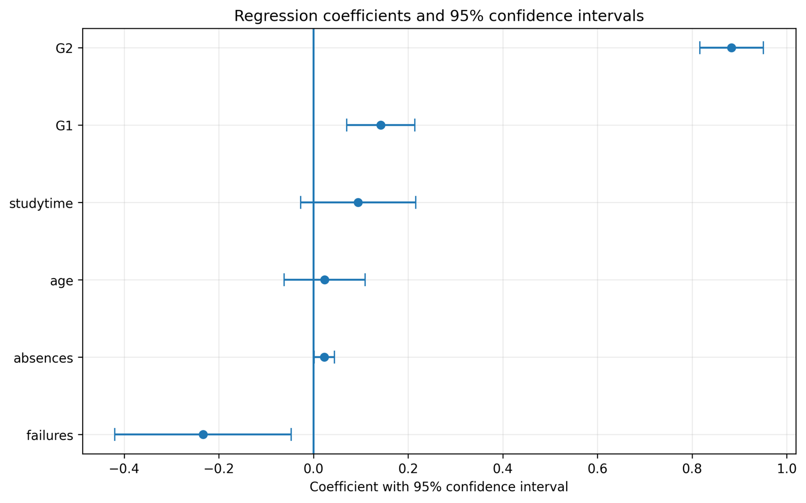
The chart compares the direction, size and uncertainty of all fitted coefficients. Intervals entirely above or below zero provide two-sided evidence against a zero coefficient at the 5% level.
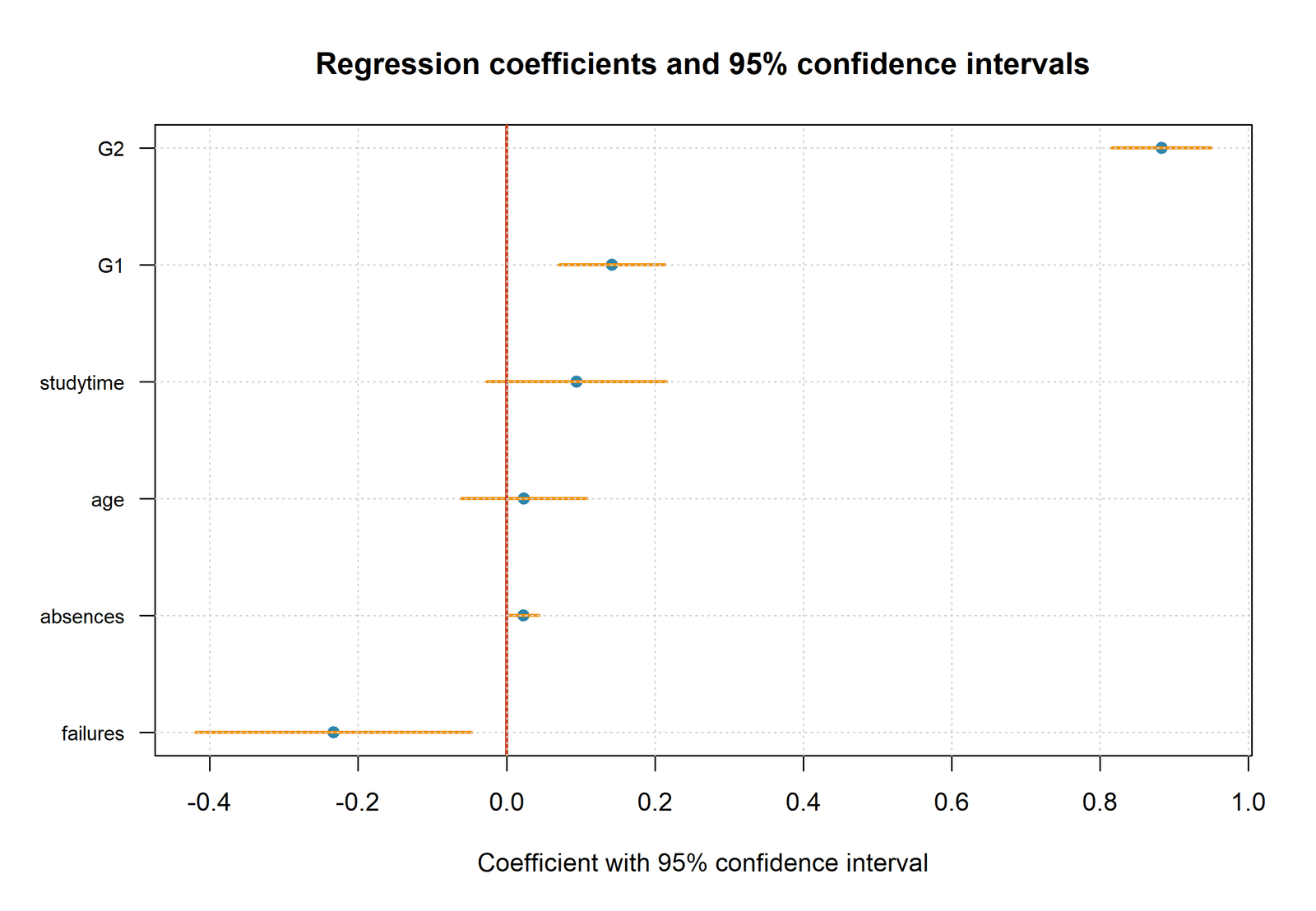
G2 has B = 0.8834 with 95% CI [0.8162, 0.9506]. G1 has B = 0.1422 with CI [0.0703, 0.2140]. Failures has B = -0.2332 with CI [-0.4196, -0.0467].
G2 is the most precisely estimated positive slope. G1 is also positive. Failures is negative. Absences has a very small positive interval, while studytime, age and the intercept cross zero.
Interpret interval width with Standard Error and Margin of Error, not with p-values alone.
Python Chart 2: Coefficient Interval Width at 90%, 95% and 99%
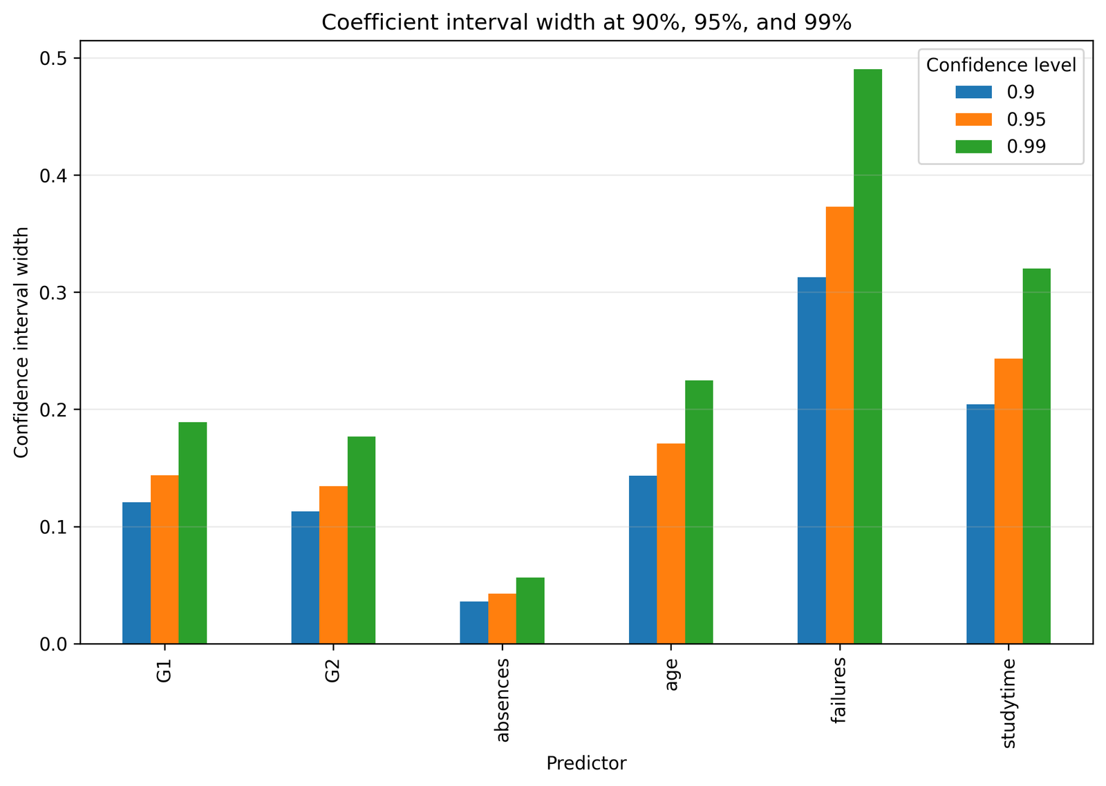
The chart demonstrates the direct trade-off between confidence level and precision. A 99% procedure must cover the true coefficient more often in repeated samples, so it needs a larger critical value and a wider interval.
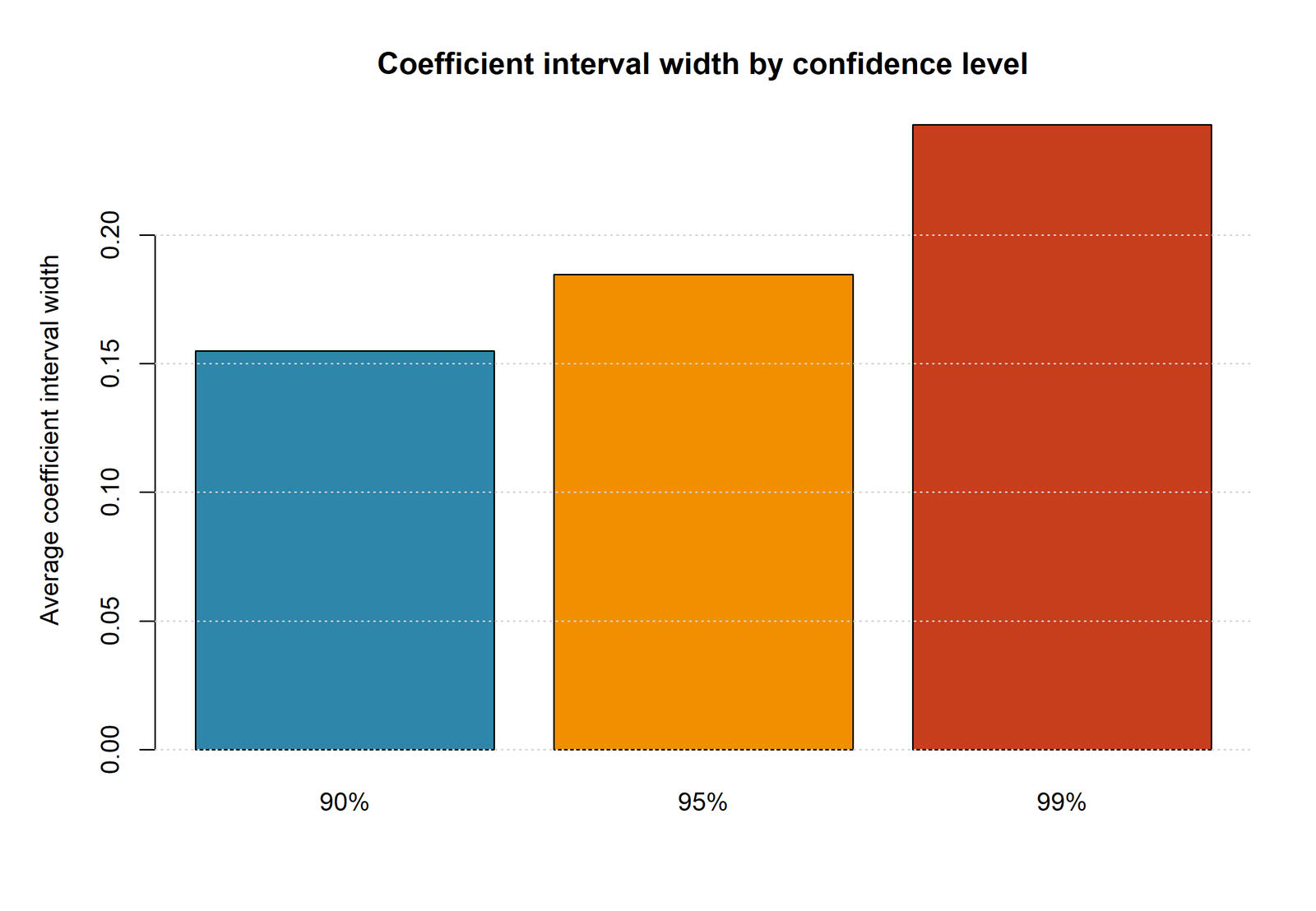
G1 width grows from 0.1205 at 90% to 0.1437 at 95% and 0.1891 at 99%. Failures grows from 0.3127 to 0.3728 and then 0.4905.
The estimate does not change when the confidence level changes. Only the uncertainty range changes. Failures and absences exclude zero at 95% but include zero at 99%, illustrating how stronger coverage requirements affect decisions.
Use the Confidence Interval guide to distinguish confidence level from the probability that one completed interval contains the parameter.
Python Chart 3: Fitted Mean with 95% Confidence Band
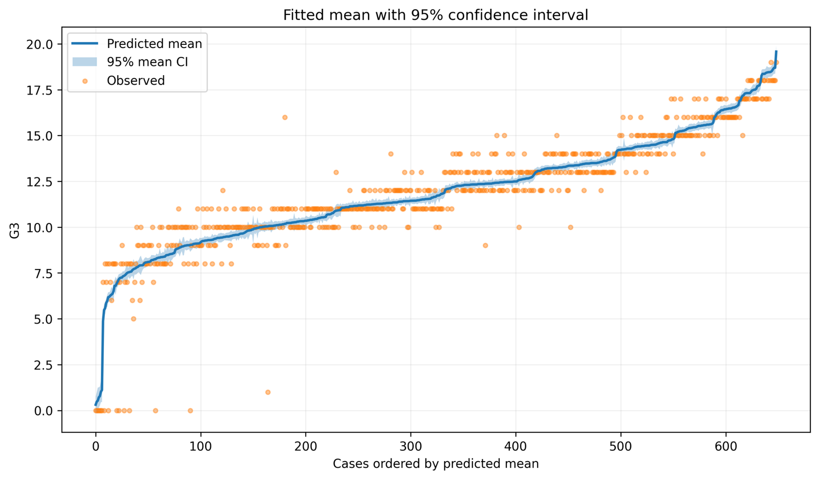
This is a confidence band for average response, not a range for one future student. It becomes wider for predictor profiles farther from the center of the design.
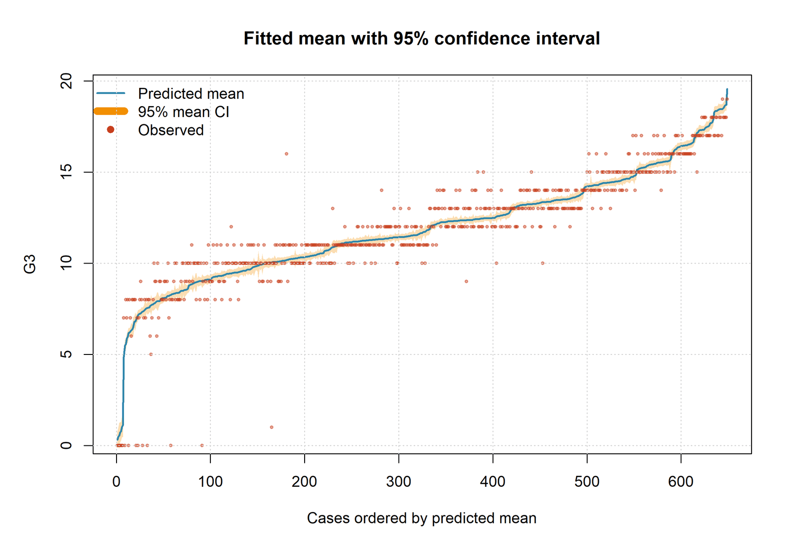
Across 649 rows, the mean-response interval has average width 0.4806 and median width 0.4371. Case 1 has an unusually wide mean interval of 1.5835.
The fitted average is estimated relatively precisely for most common profiles. Wider regions indicate higher leverage or weaker support from nearby observations.
Check unusual profiles with Influence Diagnostics and Cook’s Distance.
Python Chart 4: Individual 95% Prediction Intervals
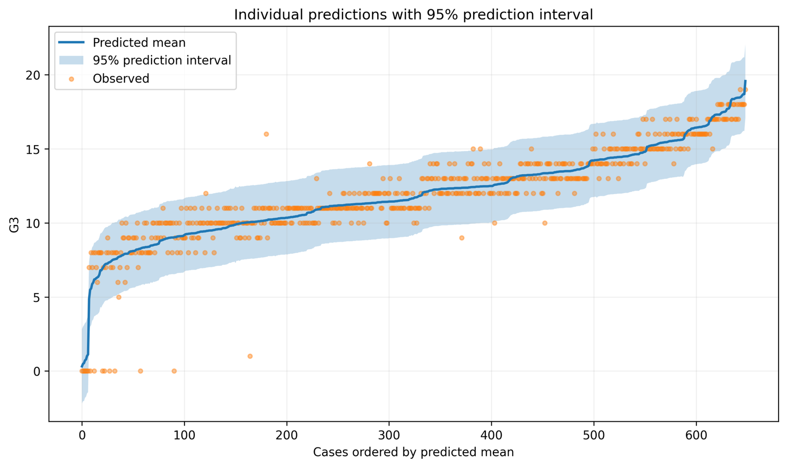
The individual limits are much wider than the fitted-mean confidence band because one new student’s outcome can vary around the conditional mean.
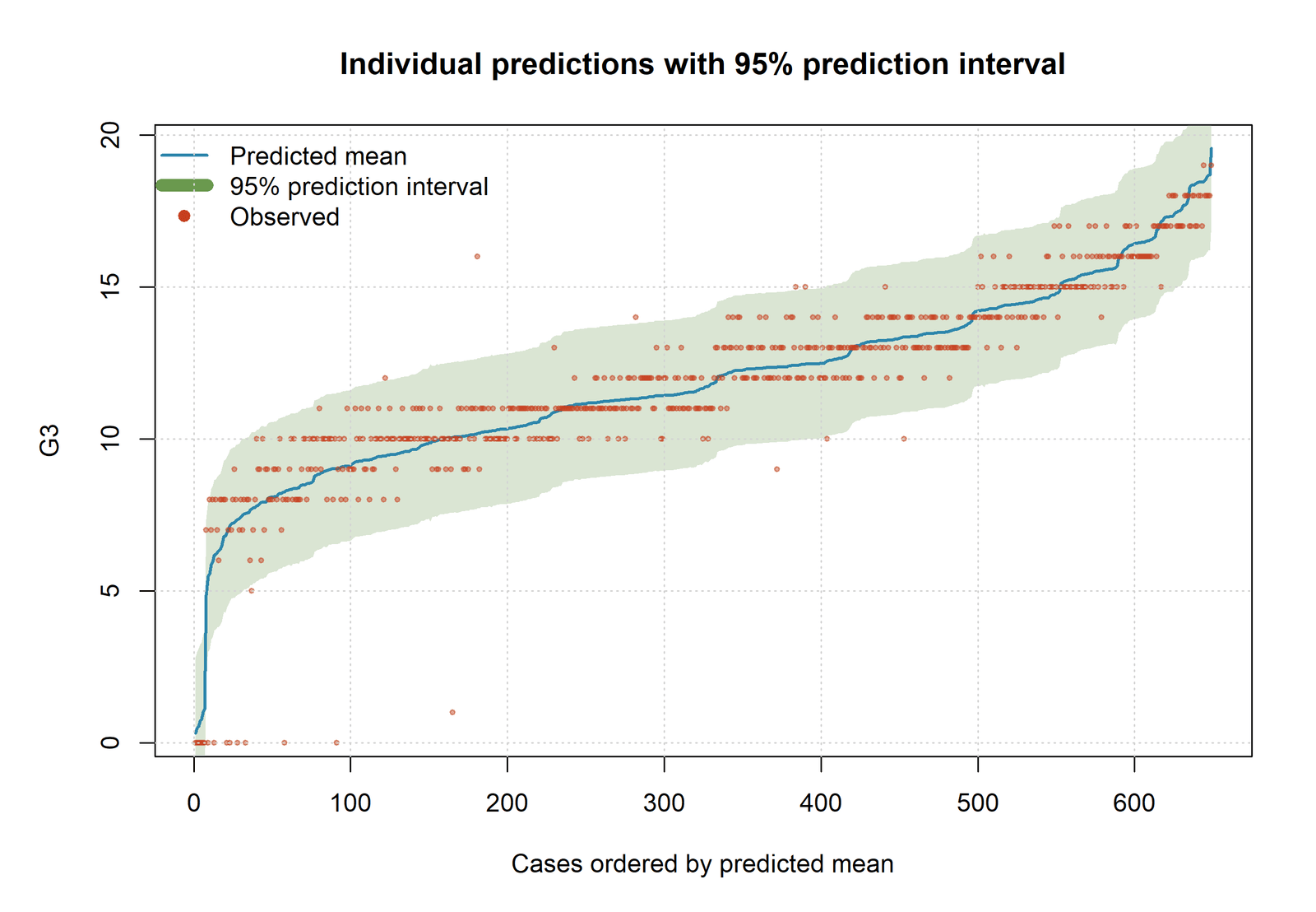
Average prediction width is 4.9529 and median width is 4.9458. Observed G3 falls inside the individual limits in 97.2265% of fitted rows.
The model estimates the average outcome with much greater precision than it predicts one individual. This is expected and is not evidence of a calculation error.
Use individual prediction intervals for case-level forecasting. Do not substitute the narrow fitted-mean band.
Python Chart 5: Observed versus Predicted G3
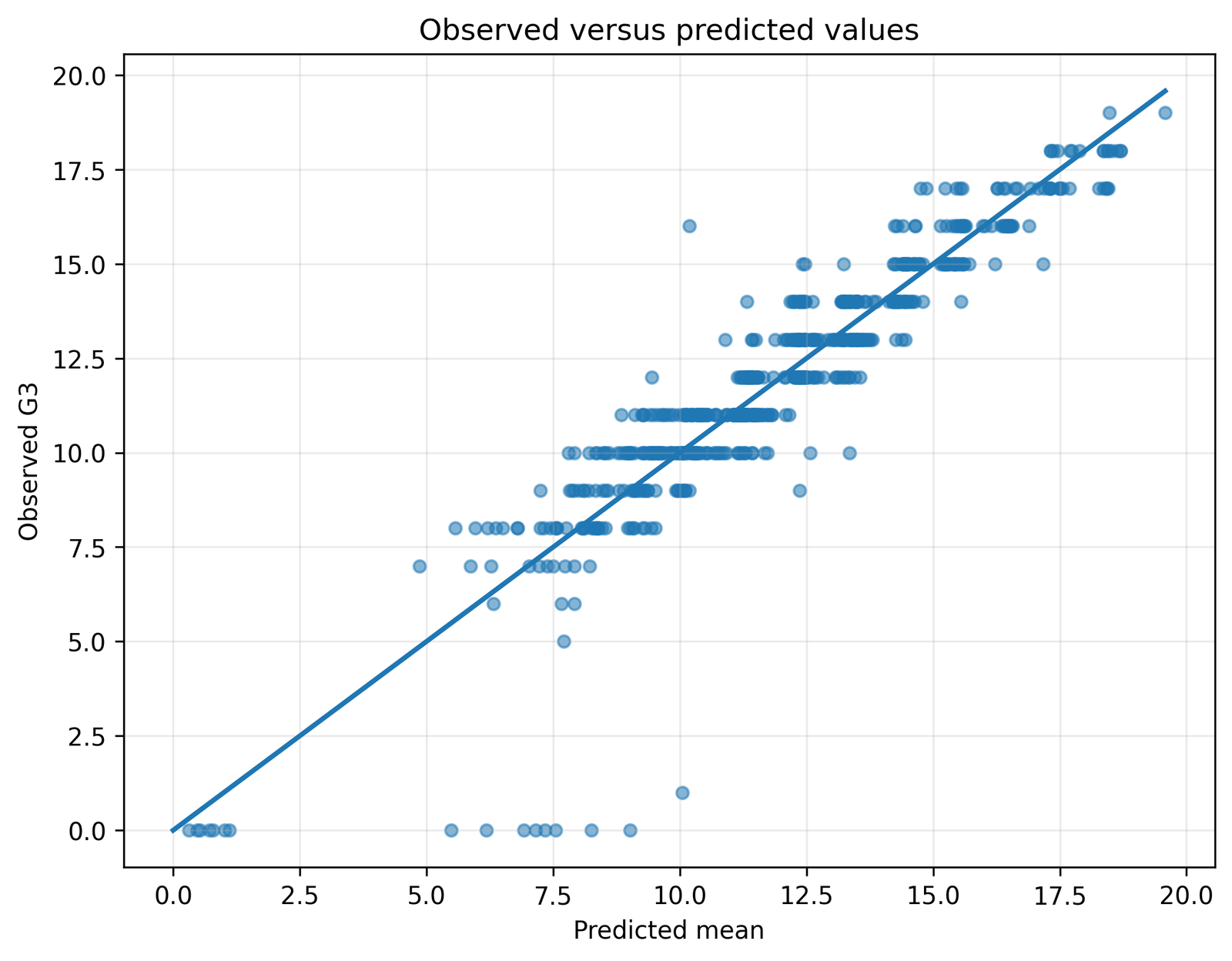
Points close to the diagonal are predicted accurately. The chart provides context for why individual residual variation must be added to prediction intervals.
The model has R² = 0.8506, adjusted R² = 0.8492, F(6,642) = 609.3527, p < .001 and residual standard error = 1.2544.
The model explains about 85.06% of observed G3 variation, but individual observations still differ from their fitted means. Strong R² therefore does not make the prediction interval unnecessary.
Review Adjusted R-Squared and Effect Size together.
Python Chart 6: Residual Evidence Behind Prediction Width
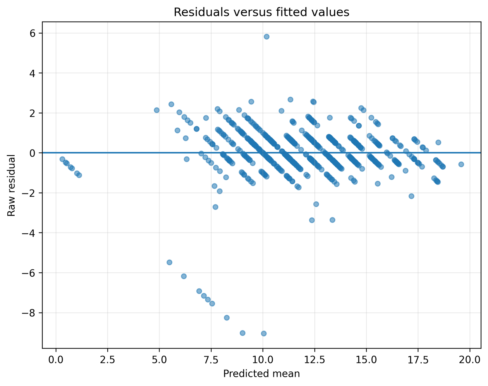
The residual plot shows how far observed G3 values fall above or below fitted means. This scatter is the main reason prediction intervals are nearly five grade points wide.
Residual standard error is 1.2544. The prediction formula adds residual variance to the leverage-based variance used for the fitted mean.
Mean-response uncertainty can be small while individual outcome uncertainty remains substantial. The two targets share the same center but not the same standard-error formula.
Inspect Studentized Residuals, Outlier Detection and residual normality.
Python Chart 7: Interval Widths across the Fitted Range
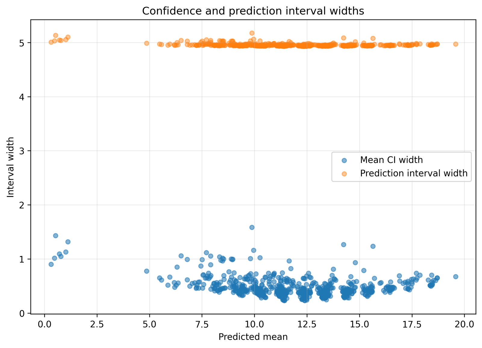
Mean interval width changes visibly with leverage. Prediction width also changes, but it remains dominated by the common residual-variance component.
Mean widths average 0.4806, while prediction widths average 4.9529. Case 1 has mean width 1.5835 and prediction width 5.1747.
A profile can be poorly supported by the design and therefore have a wider mean band. Adding residual variation makes every individual prediction interval substantially wider.
Check whether the widest intervals occur at unusual combinations of G1, G2, age, failures, absences or studytime.
Python Chart 8: Observed Inclusion by Interval Target
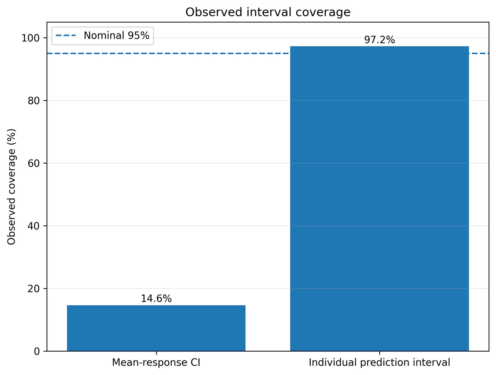
The two bars answer different questions. The first asks whether an observed individual falls inside an interval designed for the mean. The second asks whether the individual falls inside a prediction interval designed for an individual outcome.
Observed inclusion is 14.6379% for the mean-response intervals and 97.2265% for the individual prediction intervals.
The low first percentage is not failed coverage because observed individuals are not the target of a mean confidence interval. Their residual variation is included only in the prediction interval.
Report the target beside every coverage statistic so readers do not interpret mean-band inclusion as individual prediction performance.
R Charts and Explanations
The four R charts are displayed in two paired rows, followed immediately by matching explanation boxes. The mobile layout keeps each chart attached to its correct explanation.
R Chart 1: Coefficient Estimates and 95% Bounds
The R graph reproduces the positive intervals for G1 and G2, the negative interval for failures, the small positive interval for absences and zero-crossing intervals for studytime and age.
R Chart 2: Width at Three Confidence Levels
The R width chart confirms monotonic expansion from 90% to 95% to 99%. Terms with larger standard errors have larger absolute width changes.
R Chart 3: Fitted-Mean Confidence Band
The R mean-response band remains narrow near common predictor profiles and widens for higher-leverage profiles. Its average width is 0.4806.
R Chart 4: Individual Prediction Intervals
The R prediction limits are roughly five G3 points wide on average because they add residual variation to mean-estimation uncertainty.
Regression Confidence Interval Coefficient Interpretation
G2: Strong Positive Conditional Slope
Holding G1, studytime, failures, absences and age constant, one additional G2 point is associated with an expected G3 increase between approximately 0.816 and 0.951 points at the 95% confidence level.
G1: Smaller Positive Conditional Slope
G1 has a positive 95% interval from 0.070 to 0.214. The interval is wider relative to its estimate than the G2 interval, indicating lower precision.
Failures: Negative Conditional Association
The failures interval ranges from -0.420 to -0.047. At 95%, the full range is negative. At 99%, the interval widens to include zero, so the decision depends on the chosen confidence requirement.
Absences: Small Positive Estimate
The absences interval is [0.0013, 0.0440]. Although it excludes zero at 95%, the outcome-scale magnitude is small and the relationship should not be interpreted causally.
Studytime and Age
Both 95% intervals cross zero. This means the data are compatible with small negative, zero or positive conditional effects under the fitted model.
Predictions, Effects and Model Meaning
Conditional Mean versus One Future Outcome
For a fixed profile, both intervals share the same fitted center. The mean-response interval is narrow because it estimates an average. The individual prediction interval is wide because it must allow a new outcome to deviate from that average.
Worked Source Case 2
Observed G3 is 11 and fitted mean is 11.0880. The mean-response interval is [10.9015, 11.2745], while the individual prediction interval is [8.6177, 13.5583]. The observed value lies inside both.
Worked Source Case 3
Observed G3 is 12 and fitted mean is 13.3247. The mean interval is [13.1273, 13.5222], so the observed individual lies outside it. The prediction interval is [10.8536, 15.7959], so the observed individual lies inside the correct case-level range.
Why This Is Not a Contradiction
The mean interval asks where the average G3 lies for that predictor profile. It is not designed to contain every individual. The prediction interval includes residual variation and therefore answers the individual question.
Regression Confidence Interval Assumptions and Diagnostics
Evidence to inspect
- Linearity and omitted interactions
- Residual variance across fitted values
- Residual distribution and tails
- High leverage and influential observations
- Dependence or clustering
- Prediction beyond observed ranges
Why it matters
- Biased coefficients produce misleading intervals.
- Wrong standard errors produce wrong widths.
- Influential cases can shift estimates and widen bands.
- Dependence can make classical intervals too narrow.
- Out-of-range forecasts can be unstable.
- In-sample inclusion is not external validation.
Residual Normality
Use Q-Q Plot Normality Check, P-P Plot Normality Check, Shapiro-Wilk Test and Skewness and Kurtosis.
Constant Variance
Use Breusch-Pagan Test and White Test. Heteroskedasticity can invalidate classical coefficient standard errors and complicate prediction intervals.
Influence
Use Studentized Residuals, Cook’s Distance, Outlier Detection and Influence Diagnostics.
Independence
For ordered data, review Durbin-Watson Test. For clustered observations, use cluster-robust or multilevel methods rather than pretending all rows are independent.
Regression Confidence Interval in Python, R, SPSS and Excel
Python
Use statsmodels OLS and get_prediction(). The prediction summary separates mean confidence limits from observation prediction limits.
model.conf_int()for coefficientssummary_frame()for row-level bounds- Direct midpoint and width checks
- Eight diagnostic charts
R
Use confint() for coefficients and predict() with interval="confidence" or interval="prediction".
- Same formula and complete cases
- Same confidence level
- Mean and prediction targets kept separate
- Four validation charts
SPSS
Use Analyze → Regression → Linear and request coefficient confidence intervals. Save predicted values and residuals, and verify whether any exported limits target means or individuals.
- 95% coefficient intervals
- Model summary and ANOVA
- Saved predicted and residual variables
- SPSS output PDF
Excel
Excel can calculate coefficient intervals directly from B, SE and T.INV.2T. Mean and prediction intervals additionally require leverage or the design covariance matrix.
- Coefficient margin of error
- Lower and upper bounds
- Midpoint and width verification
- Design-matrix calculations for predictions
New software users can review Correlation in Python, Correlation in R, Correlation in SPSS and Correlation in Excel.
Code: Expand Only the Software You Need
Python coefficient, mean and prediction intervals
import pandas as pd
import statsmodels.api as sm

df = pd.read_csv("dataset.csv")
cols = ["G3", "G1", "G2", "studytime", "failures", "absences", "age"]
model_df = df[cols].dropna()

X = sm.add_constant(model_df[
    ["G1", "G2", "studytime", "failures", "absences", "age"]
])
y = model_df["G3"]

model = sm.OLS(y, X).fit()

coefficient_ci_95 = model.conf_int(alpha=0.05)
prediction = model.get_prediction(X).summary_frame(alpha=0.05)

# Key columns:
# mean, mean_ci_lower, mean_ci_upper
# obs_ci_lower, obs_ci_upper

prediction["mean_width"] = (
    prediction["mean_ci_upper"] - prediction["mean_ci_lower"]
)
prediction["prediction_width"] = (
    prediction["obs_ci_upper"] - prediction["obs_ci_lower"]
)
R confidence and prediction intervals
df <- read.csv("dataset.csv")
model_df <- na.omit(df[c(
  "G3", "G1", "G2", "studytime",
  "failures", "absences", "age"
)])

fit <- lm(
  G3 ~ G1 + G2 + studytime + failures + absences + age,
  data = model_df
)

confint(fit, level = 0.95)

mean_ci <- predict(
  fit,
  newdata = model_df,
  interval = "confidence",
  level = 0.95
)

prediction_interval <- predict(
  fit,
  newdata = model_df,
  interval = "prediction",
  level = 0.95
)
SPSS coefficient confidence intervals
REGRESSION
 /MISSING LISTWISE
 /STATISTICS COEFF OUTS R ANOVA CI(95)
 /DEPENDENT G3
 /METHOD=ENTER G1 G2 studytime failures absences age
 /SAVE PRED(Predicted_G3) RESID(Residual_G3).

OUTPUT SAVE
 /OUTFILE='D:\DATA ANALYSIS\H Regression Tests and Models\Regression Confidence Interval\SPSS_Output\spv\Regression-Confidence-Interval.spv'.

OUTPUT EXPORT
 /CONTENTS EXPORT=ALL LAYERS=PRINTSETTING MODELVIEWS=PRINTSETTING
 /PDF DOCUMENTFILE='D:\DATA ANALYSIS\H Regression Tests and Models\Regression Confidence Interval\SPSS_Output\pdf\Regression-Confidence-Interval-SPSS-Output.pdf'.
Excel coefficient interval formulas
Critical t:
=T.INV.2T(1-Confidence_Level, Residual_DF)

Margin of error:
=Critical_t*Coefficient_Standard_Error

Lower bound:
=Coefficient-Margin_of_Error

Upper bound:
=Coefficient+Margin_of_Error

Midpoint check:
=(Lower_Bound+Upper_Bound)/2

Width check:
=Upper_Bound-Lower_Bound
Advanced Regression Confidence Interval Topics
Expand only the technical topic needed for the current study.
Coefficient interval versus prediction interval
- A coefficient interval targets one unknown population slope.
- A prediction interval targets one future outcome.
- They use different standard-error formulas and should never be interchanged.
Mean-response confidence interval
- The mean-response interval estimates the average outcome for a fixed predictor profile.
- It contains uncertainty in the fitted regression surface.
- It does not contain ordinary person-to-person residual variation.
Frequentist meaning of 95% confidence
- The completed interval is fixed once the sample is observed.
- The 95% statement concerns long-run coverage of the method over repeated samples.
- It is not a 95% posterior probability for the fixed coefficient.
Critical t value
- The 95% two-sided critical value is 1.963665968734212 with 642 residual degrees of freedom.
- The t distribution is used because residual variance is estimated.
- As residual degrees of freedom grow, the critical value approaches the normal value 1.96.
Margin of error
- Coefficient margin of error equals critical t multiplied by coefficient standard error.
- Review Margin of Error for the arithmetic.
- The lower and upper bounds equal estimate minus and plus the margin.
Midpoint and width verification
- The midpoint of lower and upper bounds must equal the estimate.
- The interval width must equal upper minus lower.
- These two checks catch transcription and spreadsheet errors.
Why widths differ across coefficients
- Each coefficient has its own standard error.
- Standard errors depend on residual variance, sample size, predictor spread and predictor overlap.
- The same critical value therefore produces different widths.
Why widths differ across predictor profiles
- Mean-response uncertainty depends on leverage.
- Profiles near the design center are usually estimated more precisely.
- Profiles far from common combinations receive wider mean bands.
Why prediction intervals are much wider
- They contain mean-estimation variance plus residual variance.
- Residual standard error is 1.2544 in this model.
- That common residual component dominates most individual interval widths.
Why mean-band observed inclusion is low
- The mean band is not designed to contain individual observed outcomes.
- Observed outcomes include residual deviations around the mean.
- Individual prediction intervals are the correct comparison target.
Coverage versus fitted-sample inclusion
- Theoretical coverage concerns repeated future samples or outcomes under assumptions.
- The displayed 97.23% is an in-sample descriptive inclusion rate.
- It should not be treated as external validation.
Confidence level selection
- Higher confidence produces wider intervals.
- The selected level should reflect decision stakes and reporting conventions.
- Do not switch levels after seeing which terms cross zero.
Multiple intervals and multiplicity
- Seven separate 95% coefficient intervals do not provide 95% simultaneous family coverage.
- Bonferroni or simultaneous procedures may be needed for a family-wide statement.
- Distinguish individual and simultaneous inference.
Two-sided versus one-sided intervals
- The reported intervals are two-sided.
- A one-sided bound answers a different directional question.
- Choose the direction before examining results.
Robust standard errors
- Heteroskedasticity-consistent standard errors can change coefficient intervals.
- They do not change the fitted coefficients.
- They do not automatically provide correct prediction intervals.
Bootstrap intervals
- Bootstrap procedures estimate uncertainty by resampling observations.
- Percentile, basic and BCa intervals have different properties.
- The entire model and prediction calculation must be repeated in every bootstrap sample.
Bayesian credible intervals
- A credible interval has a probability interpretation conditional on the model and prior.
- It is not interchangeable with a frequentist confidence interval.
- State the inferential framework clearly.
Bounded outcome concerns
- G3 is bounded between 0 and 20 in the original educational scale.
- Linear prediction limits can extend beyond plausible boundaries.
- Report this limitation when using individual forecasts.
Residual normality
- Classical small-sample t intervals rely on normal-error assumptions.
- Large samples often provide some robustness for coefficient inference.
- Use Q-Q Plot, Shapiro-Wilk Test and Skewness and Kurtosis.
Homoscedasticity
- Constant residual variance supports the classical standard-error formulas.
- Use Breusch-Pagan Test and White Test.
- Changing variance can make classical intervals too narrow or too wide.
Independence
- The model assumes residual independence across students.
- Review Durbin-Watson Test for ordered data.
- Clustered or repeated observations need cluster-aware or multilevel inference.
Influential observations
- High-leverage cases can widen mean intervals and change coefficients.
- Use Cook’s Distance and Influence Diagnostics.
- Investigate rather than delete automatically.
Prediction for a new case
- The new row must use the same coding and predictor units.
- The fitted value is the center of both the mean and individual intervals.
- The individual interval is the appropriate uncertainty range for the new outcome.
Extrapolation
- Intervals can become misleading outside the observed predictor region.
- The linear mean function may not remain appropriate.
- State observed ranges and avoid unsupported extrapolation.
Model misspecification
- Correct interval arithmetic cannot rescue an incorrect mean function.
- Omitted nonlinearity or interactions can bias the fitted coefficients.
- Residual plots and substantive theory remain necessary.
R-squared and interval width
- A high R² does not guarantee narrow coefficient or prediction intervals.
- Interval width also depends on sample size, design geometry and residual variance.
- Read Adjusted R-Squared for model-fit interpretation.
P-values and intervals
- For a two-sided test at alpha .05, a 95% coefficient interval excludes zero exactly when p is below .05 under matching assumptions.
- Review P-Value and Null and Alternative Hypothesis.
- Intervals additionally show effect direction and precision.
Practical significance
- A narrow interval around a tiny effect can be statistically significant but practically small.
- Absences has a positive but small coefficient range.
- Use Effect Size to discuss practical magnitude.
Statistical power
- Power influences whether meaningful coefficients are estimated precisely enough to exclude zero.
- Use Statistical Power for future-study planning.
- Power planning should reflect predictor overlap and anticipated residual variance.
Type I and Type II errors
- A Type I error occurs when an interval excludes zero for a truly zero coefficient.
- A Type II error occurs when an interval includes zero despite a meaningful effect.
- Review Type I and Type II Error.
Software agreement
- Python, R and SPSS should match when formula, cases, confidence level and variance estimator match.
- Differences often arise from missing-data handling, reference coding or robust versus classical standard errors.
- Compare numerical tables rather than reading endpoints from chart pixels.
Excel calculation limits
- Excel can reproduce coefficient margins from B, SE and T.INV.2T.
- Mean and prediction intervals require leverage or design covariance.
- Adding and subtracting one residual standard error is not a valid prediction interval.
APA-Style Reporting
Publication Checklist
Always report
- The interval target
- The confidence level
- The estimate and both endpoints
- The regression formula and sample size
- Residual degrees of freedom
- The variance estimator
- Model-fit evidence
- Relevant diagnostics
- Whether coverage is in-sample or external
- Software and coding consistency
Avoid these mistakes
- Calling a prediction interval a confidence interval without naming the target
- Using a mean band for one individual
- Interpreting 95% as a posterior probability
- Ignoring profile leverage
- Reporting endpoints without the estimate
- Using p-values without effect ranges
- Comparing models with different rows
- Assuming high R² guarantees narrow prediction limits
- Ignoring heteroskedasticity
- Claiming causal effects from precise intervals
Downloads and Chart Resources
R Regression Confidence Interval ReportR validation of coefficient and fitted-response intervals
SPSS Regression Confidence Interval OutputModel summary, coefficients, confidence limits and regression output
Confidence Interval GuideContinue with the general interpretation of confidence levels and margins
Frequently Asked Questions
What is a Regression Confidence Interval?
It is an uncertainty range attached to a regression quantity such as a coefficient or a fitted mean. The target must be named explicitly.
What is the model outcome?
G3 is the continuous outcome.
How many observations are analyzed?
The model uses 649 complete cases.
How many predictors are used?
Six predictors are used: G1, G2, studytime, failures, absences and age.
What is the model R-squared?
R² is 0.8506 and adjusted R² is 0.8492.
What is the 95% critical t value?
It is 1.963665968734212 with 642 residual degrees of freedom.
What is a coefficient confidence interval?
It is a range of population slope values compatible with the estimate and its standard error under the model assumptions.
What is a fitted-mean confidence interval?
It estimates the conditional average outcome for a specified predictor profile.
What is an individual prediction interval?
It estimates a plausible range for one future outcome at a specified predictor profile.
Why is the prediction interval wider?
It adds residual outcome variance to uncertainty about the fitted mean.
What is the average fitted-mean interval width?
It is approximately 0.4806.
What is the average individual prediction width?
It is approximately 4.9529.
What is the prediction inclusion rate?
Observed G3 falls inside the fitted individual intervals for approximately 97.23% of rows.
Why is mean-band inclusion only 14.64%?
Because observed individuals are not the target of mean-response confidence intervals.
Which predictors have 95% intervals excluding zero?
G1, G2, failures and absences.
Which predictors cross zero at 95%?
The intercept, studytime and age.
Does G2 have the strongest evidence?
Yes. Its interval is narrow, positive and far from zero.
Why do failures and absences cross zero at 99%?
The 99% critical value is larger, so their intervals become wide enough to include zero.
Does a 95% interval mean a 95% probability for the coefficient?
Not in this frequentist analysis. It describes long-run coverage of the procedure.
Can I use the mean interval for a student prediction?
No. Use the individual prediction interval.
Can Excel calculate coefficient intervals?
Yes, using the coefficient, standard error and a t critical value.
Can Excel calculate mean and prediction intervals?
Yes, but it needs leverage or the design covariance matrix in addition to residual variance.
Can SPSS produce coefficient intervals?
Yes. Request confidence intervals in Linear Regression.
Can Python produce all three interval types?
Yes. statsmodels provides coefficient intervals and prediction summaries.
Can R produce all three interval types?
Yes. confint() and predict() with interval settings provide the main outputs.
What assumptions matter most?
Correct linear form, independent observations, appropriate variance treatment and a credible residual distribution.
Should unusual cases be deleted?
No. Verify and investigate them before considering any sensitivity analysis.
Do narrow intervals prove causation?
No. Precision does not establish causal identification.
What should be reported?
Report the interval target, confidence level, estimate, endpoints, model specification and relevant diagnostics.
Regression Confidence Interval Conclusion
Regression Confidence Interval reporting should combine endpoints, effect magnitude, model fit and diagnostic evidence.
Regression Confidence Interval results become misleading when a mean-response band is presented as an individual forecast.
Regression Confidence Interval width reflects both the chosen coverage level and the relevant standard-error formula.
Regression Confidence Interval interpretation should always begin by naming the exact estimand and confidence level.
Regression Confidence Interval reporting should combine endpoints, effect magnitude, model fit and diagnostic evidence.
Regression Confidence Interval results become misleading when a mean-response band is presented as an individual forecast.
Regression Confidence Interval width reflects both the chosen coverage level and the relevant standard-error formula.
Regression Confidence Interval interpretation should always begin by naming the exact estimand and confidence level.
Regression Confidence Interval reporting should combine endpoints, effect magnitude, model fit and diagnostic evidence.
Regression Confidence Interval results become misleading when a mean-response band is presented as an individual forecast.
Regression Confidence Interval width reflects both the chosen coverage level and the relevant standard-error formula.
Regression Confidence Interval interpretation should always begin by naming the exact estimand and confidence level.
Regression Confidence Interval reporting should combine endpoints, effect magnitude, model fit and diagnostic evidence.
Regression Confidence Interval results become misleading when a mean-response band is presented as an individual forecast.
Regression Confidence Interval width reflects both the chosen coverage level and the relevant standard-error formula.
Regression Confidence Interval interpretation should always begin by naming the exact estimand and confidence level.
Regression Confidence Interval reporting should combine endpoints, effect magnitude, model fit and diagnostic evidence.
Regression Confidence Interval results become misleading when a mean-response band is presented as an individual forecast.
Regression Confidence Interval width reflects both the chosen coverage level and the relevant standard-error formula.
Regression Confidence Interval interpretation should always begin by naming the exact estimand and confidence level.
Regression Confidence Interval reporting should combine endpoints, effect magnitude, model fit and diagnostic evidence.
Regression Confidence Interval results become misleading when a mean-response band is presented as an individual forecast.
Regression Confidence Interval width reflects both the chosen coverage level and the relevant standard-error formula.
Regression Confidence Interval interpretation should always begin by naming the exact estimand and confidence level.
Regression Confidence Interval reporting should combine endpoints, effect magnitude, model fit and diagnostic evidence.
Regression Confidence Interval results become misleading when a mean-response band is presented as an individual forecast.
Regression Confidence Interval width reflects both the chosen coverage level and the relevant standard-error formula.
Regression Confidence Interval interpretation should always begin by naming the exact estimand and confidence level.
Regression Confidence Interval reporting should combine endpoints, effect magnitude, model fit and diagnostic evidence.
Regression Confidence Interval results become misleading when a mean-response band is presented as an individual forecast.
Regression Confidence Interval width reflects both the chosen coverage level and the relevant standard-error formula.
Regression Confidence Interval interpretation should always begin by naming the exact estimand and confidence level.
Regression Confidence Interval reporting should combine endpoints, effect magnitude, model fit and diagnostic evidence.
Regression Confidence Interval results become misleading when a mean-response band is presented as an individual forecast.
Regression Confidence Interval width reflects both the chosen coverage level and the relevant standard-error formula.
Regression Confidence Interval interpretation should always begin by naming the exact estimand and confidence level.
Regression Confidence Interval reporting should combine endpoints, effect magnitude, model fit and diagnostic evidence.
Regression Confidence Interval results become misleading when a mean-response band is presented as an individual forecast.
Regression Confidence Interval width reflects both the chosen coverage level and the relevant standard-error formula.
Regression Confidence Interval interpretation should always begin by naming the exact estimand and confidence level.
Regression Confidence Interval reporting should combine endpoints, effect magnitude, model fit and diagnostic evidence.
Regression Confidence Interval results become misleading when a mean-response band is presented as an individual forecast.
Regression Confidence Interval width reflects both the chosen coverage level and the relevant standard-error formula.
Regression Confidence Interval interpretation should always begin by naming the exact estimand and confidence level.
Regression Confidence Interval reporting should combine endpoints, effect magnitude, model fit and diagnostic evidence.
Regression Confidence Interval results become misleading when a mean-response band is presented as an individual forecast.
Regression Confidence Interval width reflects both the chosen coverage level and the relevant standard-error formula.
Regression Confidence Interval interpretation should always begin by naming the exact estimand and confidence level.
Regression Confidence Interval reporting should combine endpoints, effect magnitude, model fit and diagnostic evidence.
Regression Confidence Interval results become misleading when a mean-response band is presented as an individual forecast.
Regression Confidence Interval width reflects both the chosen coverage level and the relevant standard-error formula.
Regression Confidence Interval interpretation should always begin by naming the exact estimand and confidence level.
Regression Confidence Interval reporting should combine endpoints, effect magnitude, model fit and diagnostic evidence.
Regression Confidence Interval results become misleading when a mean-response band is presented as an individual forecast.
Regression Confidence Interval width reflects both the chosen coverage level and the relevant standard-error formula.
Regression Confidence Interval interpretation should always begin by naming the exact estimand and confidence level.
Regression Confidence Interval reporting should combine endpoints, effect magnitude, model fit and diagnostic evidence.
Regression Confidence Interval results become misleading when a mean-response band is presented as an individual forecast.
Regression Confidence Interval width reflects both the chosen coverage level and the relevant standard-error formula.
Regression Confidence Interval interpretation should always begin by naming the exact estimand and confidence level.
Regression Confidence Interval reporting should combine endpoints, effect magnitude, model fit and diagnostic evidence.
Regression Confidence Interval results become misleading when a mean-response band is presented as an individual forecast.
Regression Confidence Interval width reflects both the chosen coverage level and the relevant standard-error formula.
Regression Confidence Interval interpretation should always begin by naming the exact estimand and confidence level.
Regression Confidence Interval reporting should combine endpoints, effect magnitude, model fit and diagnostic evidence.
Regression Confidence Interval results become misleading when a mean-response band is presented as an individual forecast.
Regression Confidence Interval width reflects both the chosen coverage level and the relevant standard-error formula.
Regression Confidence Interval interpretation should always begin by naming the exact estimand and confidence level.
Regression Confidence Interval reporting should combine endpoints, effect magnitude, model fit and diagnostic evidence.
Regression Confidence Interval results become misleading when a mean-response band is presented as an individual forecast.
Regression Confidence Interval width reflects both the chosen coverage level and the relevant standard-error formula.
Regression Confidence Interval interpretation should always begin by naming the exact estimand and confidence level.
Regression Confidence Interval reporting should combine endpoints, effect magnitude, model fit and diagnostic evidence.
Regression Confidence Interval results become misleading when a mean-response band is presented as an individual forecast.
Regression Confidence Interval width reflects both the chosen coverage level and the relevant standard-error formula.
Regression Confidence Interval interpretation should always begin by naming the exact estimand and confidence level.
Regression Confidence Interval reporting should combine endpoints, effect magnitude, model fit and diagnostic evidence.
Regression Confidence Interval results become misleading when a mean-response band is presented as an individual forecast.
Regression Confidence Interval width reflects both the chosen coverage level and the relevant standard-error formula.
Regression Confidence Interval interpretation should always begin by naming the exact estimand and confidence level.
Regression Confidence Interval reporting should combine endpoints, effect magnitude, model fit and diagnostic evidence.
Regression Confidence Interval results become misleading when a mean-response band is presented as an individual forecast.
Regression Confidence Interval width reflects both the chosen coverage level and the relevant standard-error formula.
Regression Confidence Interval interpretation should always begin by naming the exact estimand and confidence level.
Regression Confidence Interval reporting should combine endpoints, effect magnitude, model fit and diagnostic evidence.
Regression Confidence Interval results become misleading when a mean-response band is presented as an individual forecast.
Regression Confidence Interval width reflects both the chosen coverage level and the relevant standard-error formula.
Regression Confidence Interval interpretation should always begin by naming the exact estimand and confidence level.
Regression Confidence Interval reporting should combine endpoints, effect magnitude, model fit and diagnostic evidence.
Regression Confidence Interval results become misleading when a mean-response band is presented as an individual forecast.
Regression Confidence Interval width reflects both the chosen coverage level and the relevant standard-error formula.
Regression Confidence Interval interpretation should always begin by naming the exact estimand and confidence level.
Regression Confidence Interval reporting should combine endpoints, effect magnitude, model fit and diagnostic evidence.
Regression Confidence Interval results become misleading when a mean-response band is presented as an individual forecast.
Regression Confidence Interval width reflects both the chosen coverage level and the relevant standard-error formula.
Regression Confidence Interval interpretation should always begin by naming the exact estimand and confidence level.
Regression Confidence Interval reporting should combine endpoints, effect magnitude, model fit and diagnostic evidence.
Regression Confidence Interval results become misleading when a mean-response band is presented as an individual forecast.
Regression Confidence Interval width reflects both the chosen coverage level and the relevant standard-error formula.
Regression Confidence Interval interpretation should always begin by naming the exact estimand and confidence level.
Regression Confidence Interval analysis is most useful when it prevents three different uncertainty targets from being mixed together. Coefficient intervals describe population slopes, fitted-mean intervals describe conditional averages and prediction intervals describe one future outcome.
In this six-predictor G3 model, coefficient estimates for G1, G2, failures and absences have 95% intervals excluding zero. Mean responses are estimated relatively precisely, with average interval width 0.4806, while individual outcomes remain much more uncertain, with average prediction width 4.9529.
The central lesson is that a narrow mean band does not imply a narrow individual forecast. Correct interpretation requires the target, formula, confidence level, model assumptions and diagnostic evidence to remain aligned.

