
Regression ANOVA Table: Formula, Interpretation, Python, R, SPSS and Excel Guide
A Regression ANOVA Table partitions total variation in a continuous outcome into variation explained by the fitted regression model and variation left in the residuals. This worked guide reconstructs every row for a five-predictor model of G3 using 649 complete observations.
5 predictors
R² 0.850563
F(5, 643) = 731.966
Regression ANOVA Table Model Overview
What this method is: a Regression ANOVA Table is the standard sums-of-squares summary for an ordinary least squares regression. It separates the observed variation in a continuous dependent variable into an explained component attributed to the fitted model and an unexplained component attributed to residual error. The same table then converts those sums of squares into mean squares and an omnibus F statistic.
Definition of a Regression ANOVA Table
The word ANOVA means analysis of variance. In a regression setting, the Regression ANOVA Table does not require categorical groups. Instead, it analyses variation around the outcome mean and asks whether a set of regression predictors collectively reduces squared prediction error relative to an intercept-only model.
The table normally contains three rows:
- Regression or Model: variation explained by the fitted predictors.
- Residual or Error: variation remaining between observed and fitted outcomes.
- Total: original outcome variation around the sample mean.
For an ordinary regression fitted with an intercept, the accounting identity is exact:
Here, SST is total sum of squares, SSR is regression sum of squares, and SSE is residual or error sum of squares.
What Question Does the Regression ANOVA Table Answer?
The omnibus question is whether the complete predictor set explains more outcome variation than an intercept-only model. For the current model, the null hypothesis is:
The alternative is that at least one of those five slopes differs from zero. The F test is collective. It does not state that every predictor is important, and it does not identify which coefficient drives the rejection.
When a Regression ANOVA Table Is Used
A Regression ANOVA Table is used with Ordinary Least Squares Regression when the outcome is continuous and the model contains one or more predictors. It appears in simple linear regression, Multiple Linear Regression, hierarchical regression, polynomial regression, and many other models estimated by least squares.
The table is especially useful when readers need to reconstruct R², compare explained with unexplained variation, verify degrees of freedom, or understand the overall F test. It is also a valuable audit because several reported statistics must reconcile mathematically.
Regression ANOVA Table Versus One-Way ANOVA
One-way ANOVA compares group means using categorical predictors. A Regression ANOVA Table can include continuous predictors such as G1 and G2, discrete predictors such as failures, and coded categorical predictors. Both methods use sums of squares and F ratios because classical ANOVA is itself a linear model.
The interpretation of the model row depends on the design. In one-way ANOVA, it represents between-group variation. In multiple regression, it represents the reduction in squared error produced by the complete fitted predictor set.
Regression ANOVA Table Versus the Coefficient Table
The Regression ANOVA Table asks whether the predictor block matters collectively. The coefficient table asks about each conditional slope while the remaining predictors are held constant. A model can have a highly significant omnibus F test while one or more individual coefficients remain nonsignificant.
That is exactly what happens here. The overall model is overwhelmingly significant, but studytime has p = .1182. G1, G2, failures, and absences show stronger individual evidence.
Core Formulas
Degrees of Freedom
With n observations and p slope predictors:
- Regression df = p
- Error df = n − p − 1
- Total df = n − 1
For 649 observations and five predictors, regression df = 5, error df = 643, and total df = 648. The degrees of freedom also reconcile exactly: 5 + 643 = 648.
How the Regression ANOVA Table Connects to R-Squared
R² is the proportion of total squared variation allocated to the regression row:
In this analysis, R² = 5752.587287722169 / 6763.2665639445295 = 0.8505634419896496. Therefore, the fitted model accounts for approximately 85.06% of the observed G3 variation around its mean.
Adjusted R-Squared is 0.849401415877594 after accounting for five predictors and the sample size. It is close to R² because the model’s explained variation is large relative to the number of predictors.
What the F Statistic Means
The F statistic compares explained variation per regression degree of freedom with unexplained variation per error degree of freedom. The numerator mean square is 1150.517457544434, and the denominator mean square is 1.571818470019223. Their ratio is 731.9658596010539.
An F value this large means that the average explained square per predictor degree of freedom is hundreds of times larger than the average residual square per error degree of freedom. The associated p-value is approximately 1.33 × 10−262, so the collective null is rejected.
Assumptions Behind the Reference F Distribution
The sums-of-squares identity is arithmetic, but the classical p-value relies on a suitable linear model. Important conditions include an adequate linear mean structure, independent errors, approximately constant conditional variance, no severe influential-case distortion, and an error distribution suitable for the intended inference.
Normality is most relevant for exact finite-sample tests and confidence intervals. With 649 observations, asymptotic robustness is substantial, but extreme residuals and heteroskedasticity can still affect conventional standard errors and the MSE denominator.
Advantages of the Regression ANOVA Table
- Provides a complete audit of explained, residual, and total variation.
- Connects R² directly to sums of squares.
- Produces the omnibus F test for the predictor block.
- Reconciles degrees of freedom and model error.
- Can be reproduced in Python, R, SPSS, and Excel.
- Helps detect inconsistent or incorrectly copied model summaries.
Limitations
- The table does not identify which predictor is responsible for model significance.
- It does not establish causal contribution.
- It does not diagnose nonlinearity, unequal variance, dependence, or influential observations by itself.
- Sequential and partial sums of squares can differ in more complex designs.
- A large F statistic does not guarantee good prediction on future data.
- A high R² does not make every individual prediction accurate.
Current Worked Scenario
The dependent variable is G3. The predictors are G1, G2, studytime, failures, and absences. All 649 observations are complete for the fitted model. The regression sum of squares is 5752.587287722169, residual sum of squares is 1010.6792762223604, and total sum of squares is 6763.2665639445295.
The model has F(5, 643) = 731.9658596010539, p < .001, R² = 0.8505634419896496, adjusted R² = 0.849401415877594, and RMSE = 1.2537218471492084.
Quick Answer
Three-row decomposition
- Regression: SS = 5752.5873, df = 5, MS = 1150.5175
- Error: SS = 1010.6793, df = 643, MS = 1.571818
- Total: SS = 6763.2666, df = 648
Best one-sentence interpretation
- The five predictors collectively explain approximately 85.06% of G3 variation.
- The omnibus test is F(5, 643) = 731.97, p < .001.
- The overall result does not imply that every slope is significant.
Table of Contents
- Why this analysis needs a Regression ANOVA Table
- How the Regression ANOVA Table works
- Variables and data dictionary
- Complete Regression ANOVA Table results
- Eight Python chart stories
- Four R charts and explanations
- Coefficient interpretation
- Predictions and residual contributions
- Assumptions and diagnostics
- Python, R, SPSS and Excel workflows
- Code
- Advanced Regression ANOVA Table topics
- APA-style reporting
- Publication checklist
- Downloads
- Related Salar Cafe guides
- Frequently asked questions
Why This Analysis Needs a Regression ANOVA Table
The worked question is not merely whether one coefficient differs from zero. It asks how much total variation is explained by the complete five-predictor equation and whether that explained component is large relative to residual variation.
A coefficient-only summary cannot answer that question because each slope is conditional on the others. The Regression ANOVA Table provides a model-wide test and then connects the result to R² and RMSE.
The table is also an integrity check. If SSR + SSE does not reproduce SST, if the degrees of freedom do not add correctly, or if MSR / MSE does not reproduce F, then the reported model summary contains an error.
The Regression ANOVA Table is particularly helpful when comparing hierarchical blocks. In those designs, the change in regression sum of squares measures how much an added block improves fit beyond predictors already entered.
How the Regression ANOVA Table Works
Square each G3 deviation from the sample mean and add the results.
Separate fitted variation from residual squared error.
Divide model mean square by error mean square.
Step 1: Total Sum of Squares
SST measures the outcome variation before the predictors are used. It is the squared-error total from predicting every student with the sample mean G3 of 11.906009244992296.
Step 2: Regression Sum of Squares
SSR measures how far fitted values vary around the outcome mean. It is the improvement attributable to the complete fitted equation, not a causal allocation to individual predictors.
Step 3: Error Sum of Squares
SSE contains every squared residual. Observations with unusually large prediction errors can contribute heavily because residuals are squared.
Step 4: Degrees of Freedom
The intercept consumes one fitted parameter but does not add a regression-row degree of freedom under the standard table. The five slopes create the five numerator degrees of freedom.
Step 5: Mean Squares
MSE is the pooled residual variance estimate under the classical model. Its square root is RMSE:
Step 6: F Statistic and P-Value
The upper-tail probability from the F Distribution with 5 and 643 degrees of freedom is approximately 1.33 × 10−262. At α = .05, the overall regression null is rejected.
Step 7: Reconstruct R-Squared
This second route verifies the reported R² independently of the software summary. The same value also equals 1 − SSE/SST.
Regression ANOVA Table and Sums-of-Squares Types
For a single full regression block, the model-versus-error decomposition is unique. When predictors are entered sequentially or when a design includes interactions and unequal groups, Type I Sum of Squares, Type II Sum of Squares, and Type III Sum of Squares answer different partial questions. The overall full-model SSR remains the reduction from the intercept-only model.
Variables and Data Dictionary
| Variable | Role | Count | Mean | SD | Range | Interpretive role |
|---|---|---|---|---|---|---|
| G3 | Outcome | 649 | 11.9060 | 3.2307 | 0–19 | Final grade whose variation is decomposed by the Regression ANOVA Table |
| G1 | Predictor | 649 | 11.3991 | 2.7453 | 0–19 | First-period grade |
| G2 | Predictor | 649 | 11.5701 | 2.9136 | 0–19 | Second-period grade and dominant conditional predictor |
| studytime | Predictor | 649 | 1.9307 | 0.8295 | 1–4 | Weekly study-time category |
| failures | Predictor | 649 | 0.2219 | 0.5932 | 0–3 | Number of previous class failures |
| absences | Predictor | 649 | 3.6595 | 4.6408 | 0–32 | Absence count |
The fitted model is:
All predictors enter simultaneously. The coefficient for each predictor is therefore conditional on the remaining four predictors. No standardization was applied to the reported coefficient table, so slopes remain in original variable units.
Complete Regression ANOVA Table Results
Explained squared variation
Residual squared variation
Original G3 variation
df = 5, 643
85.06% explained
G3 outcome units
| Source | Sum of squares | df | Mean square | F | p |
|---|---|---|---|---|---|
| Regression | 5752.587287722169 | 5 | 1150.517457544434 | 731.9658596010539 | 1.3257355956912994 × 10−262 |
| Residual / Error | 1010.6792762223604 | 643 | 1.571818470019223 | — | — |
| Total | 6763.2665639445295 | 648 | — | — | — |
Arithmetic Reconciliation
- 5752.587287722169 + 1010.6792762223604 = 6763.2665639445295
- 5 + 643 = 648
- 5752.587287722169 / 5 = 1150.517457544434
- 1010.6792762223604 / 643 = 1.571818470019223
- 1150.517457544434 / 1.571818470019223 = 731.9658596010539
- 5752.587287722169 / 6763.2665639445295 = 0.8505634419896496
Statistical Decision
The Regression ANOVA Table rejects the null hypothesis that all five slopes are zero, F(5, 643) = 731.97, p < .001. The fitted model provides substantially better predictions than the outcome mean alone.
The result is statistically decisive, but practical interpretation should include the original-unit error. RMSE is approximately 1.254 G3 points, so the model can explain most variation while still making important case-level errors.
Open the Verified Output Files
The reports and workbook contain the complete source calculations supporting this Regression ANOVA Table.
Eight Python Chart Stories
The Python figures connect the Regression ANOVA Table to observed predictions, residual behavior, coefficient evidence, and the original-unit error scale.
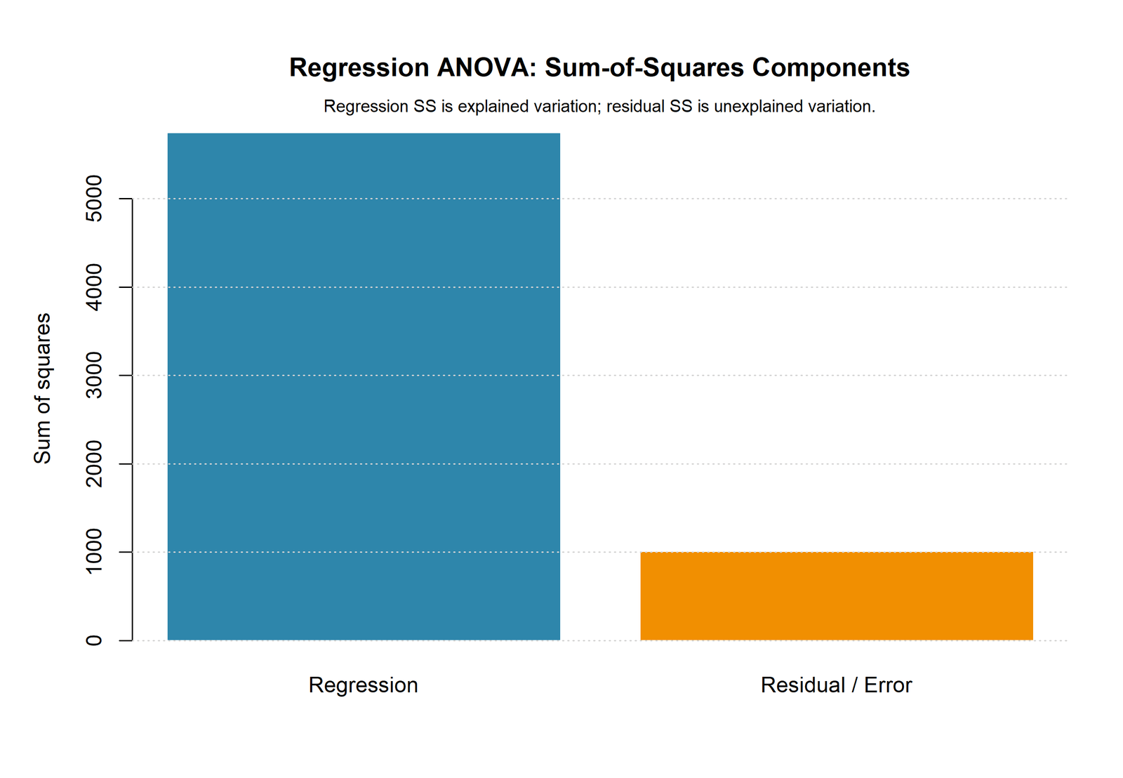
Python Chart 1: Sum-of-Squares Partition
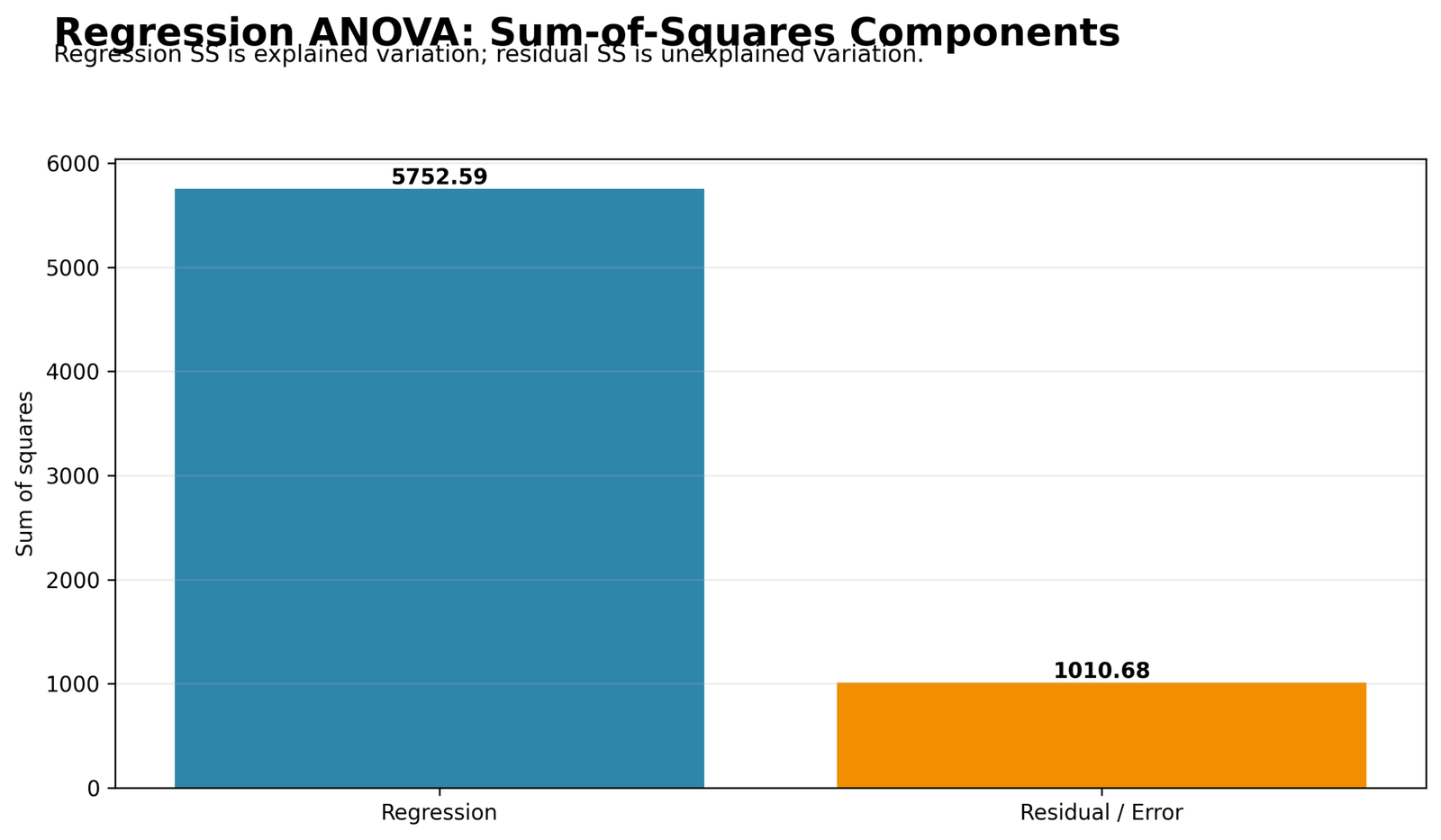
The explained component occupies most of the total, while the residual component remains substantial enough to require diagnostic review.
SSR = 5752.5873, SSE = 1010.6793, and SST = 6763.2666. SSR represents 85.0563% of SST; SSE represents 14.9437%.
The model captures most squared variation around mean G3. The bars are complementary parts of one fixed total, not independent effect sizes that can be attributed to separate predictors.
This figure provides the fastest visual audit of the Regression ANOVA Table and connects directly to R².
Python Chart 2: Observed Versus Fitted G3
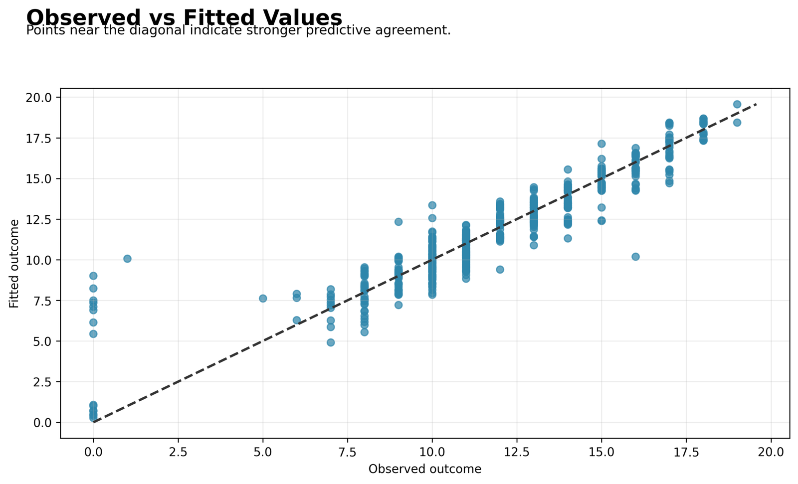
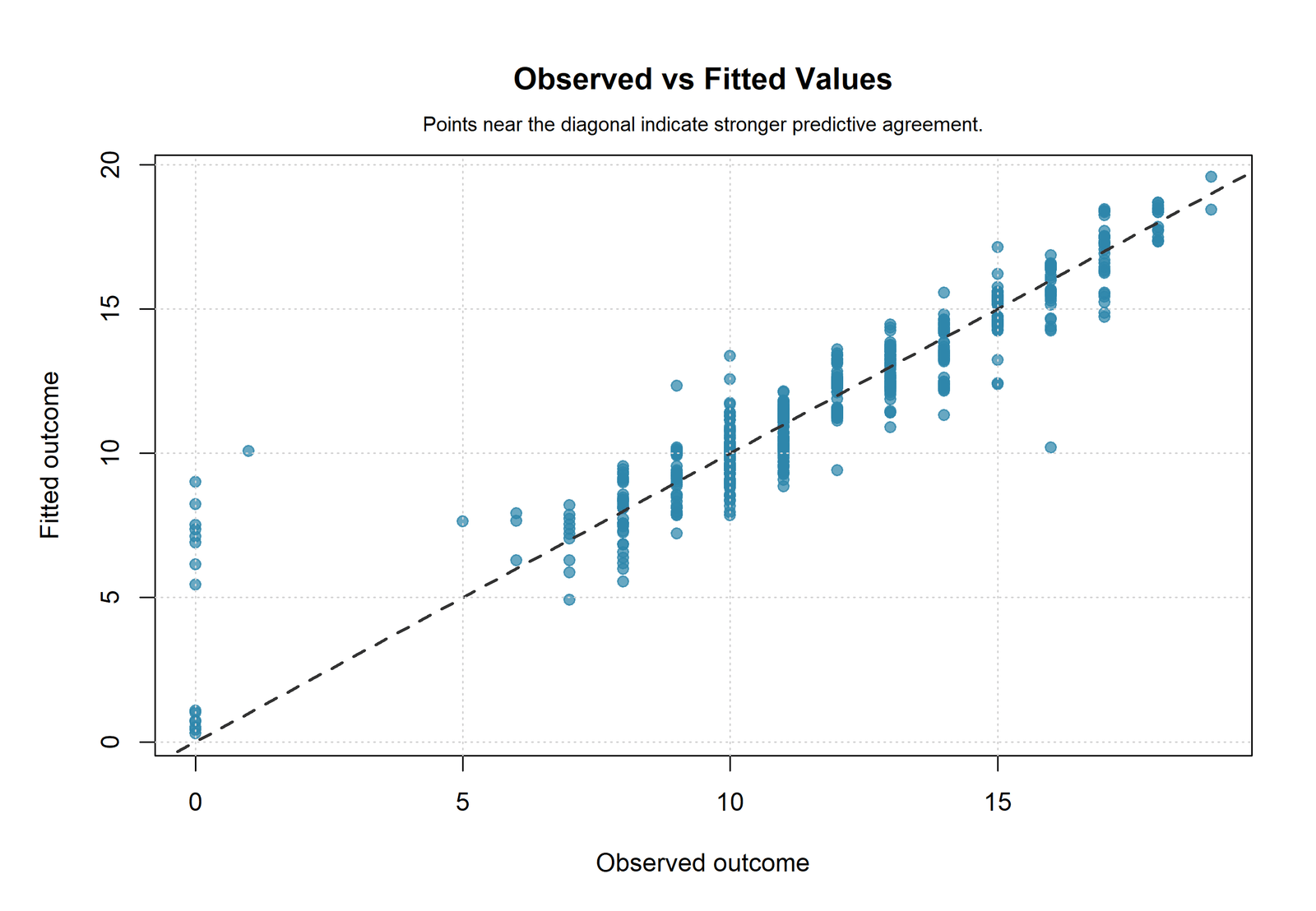
Most observations follow the agreement line through the central and upper ranges. A smaller group of very low observed grades receives substantially higher fitted values.
R² = 0.850563, adjusted R² = 0.849401, and RMSE = 1.253722. The fitted-value mean equals the observed mean, 11.906009.
Close alignment explains the large regression sum of squares. Large vertical distances identify observations that contribute disproportionately to SSE.
A model-wide F test can be extremely strong while a small group of observations remains poorly predicted.
Python Chart 3: Residuals Versus Fitted Values
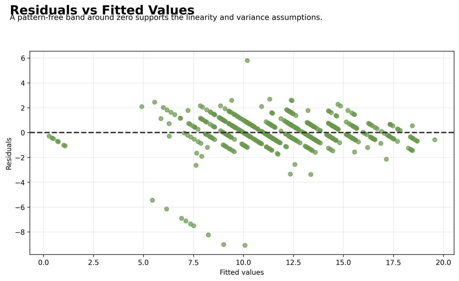
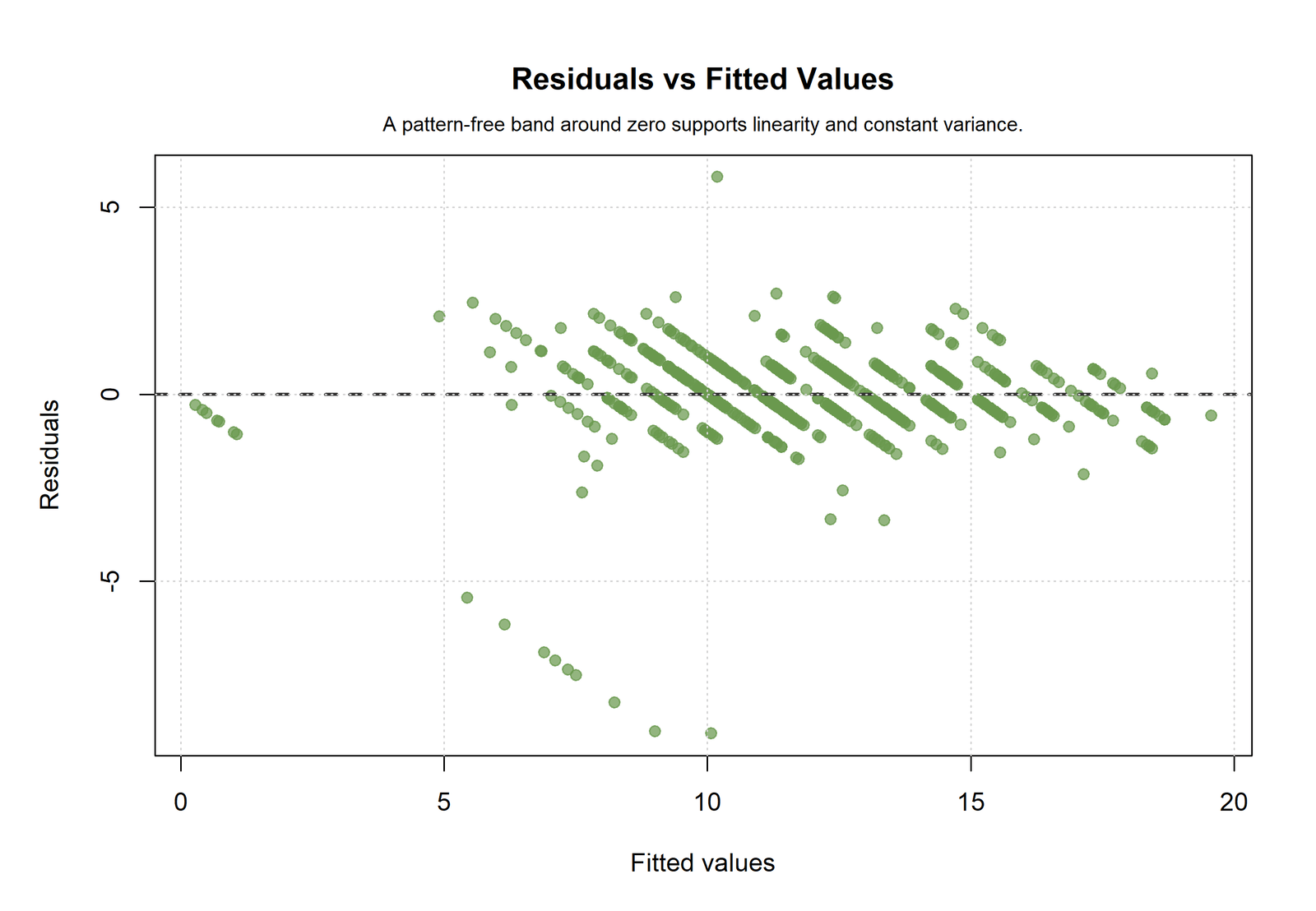
The central residual cloud remains close to zero without a dominant smooth curve. Diagonal bands arise because observed G3 is recorded in integer units, while fitted values are continuous.
The residual median is approximately −0.0796. About 78.3% of absolute residuals are within 1 point and 95.7% are within 2 points.
The mean structure captures the main relationship, but several large negative residuals create a long lower tail. A strong funnel would challenge constant variance; the visible concern here is concentrated extreme error rather than a universal spread increase.
This plot should be reviewed with Breusch-Pagan Test and White Test concepts rather than treating the pooled MSE as automatically valid everywhere.
Python Chart 4: Residual Distribution
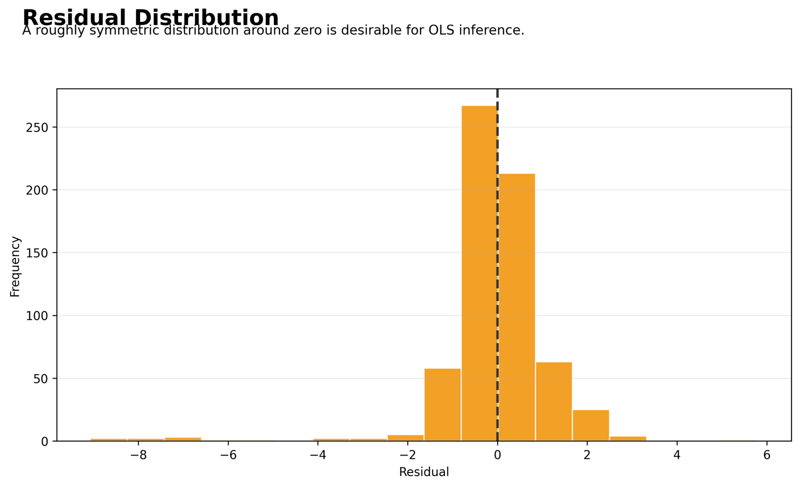
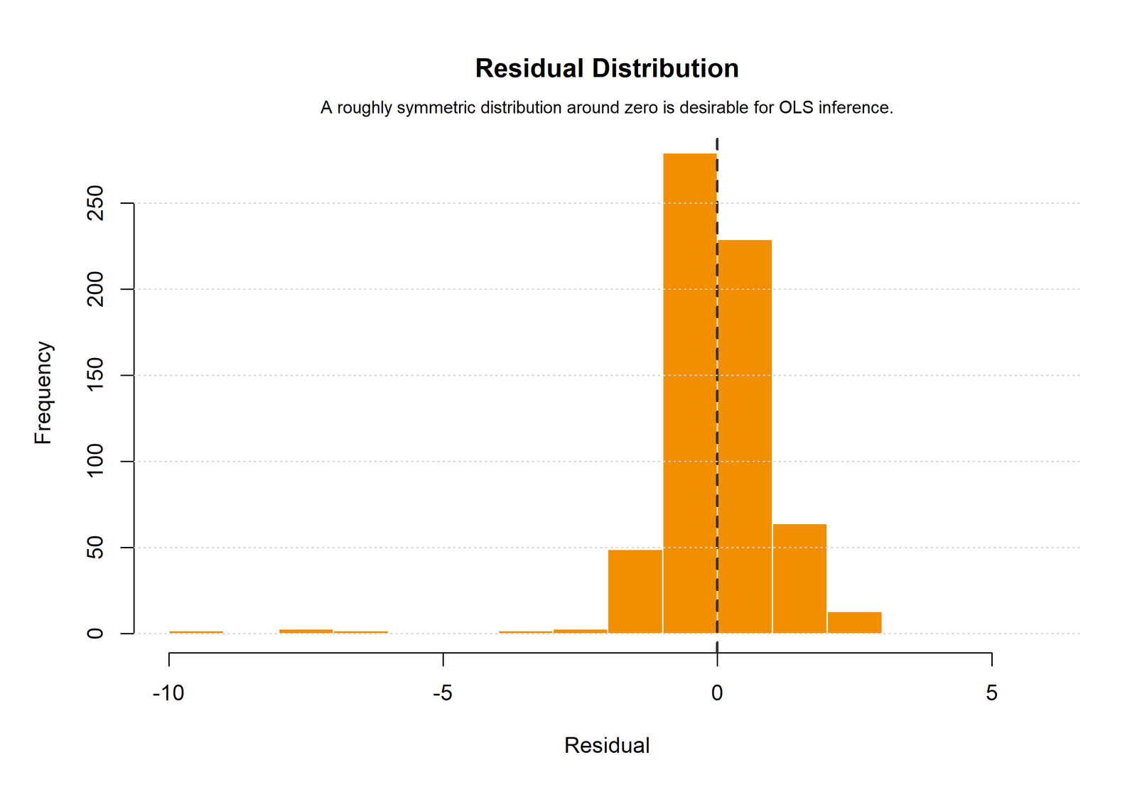
Most residuals are tightly concentrated near zero, but the negative tail extends farther than the positive tail because several zero or near-zero outcomes are overpredicted.
Residual Q1 = −0.4624, median = −0.0796, Q3 = 0.6346, minimum = −9.0716, and maximum = 5.8068.
The central distribution supports the model’s low RMSE, while the asymmetric tail shows why average fit statistics must not replace case-level review.
Because SSE squares each error, a few extreme residuals can contribute far more than many ordinary residuals.
Python Chart 5: Normal Q-Q Plot
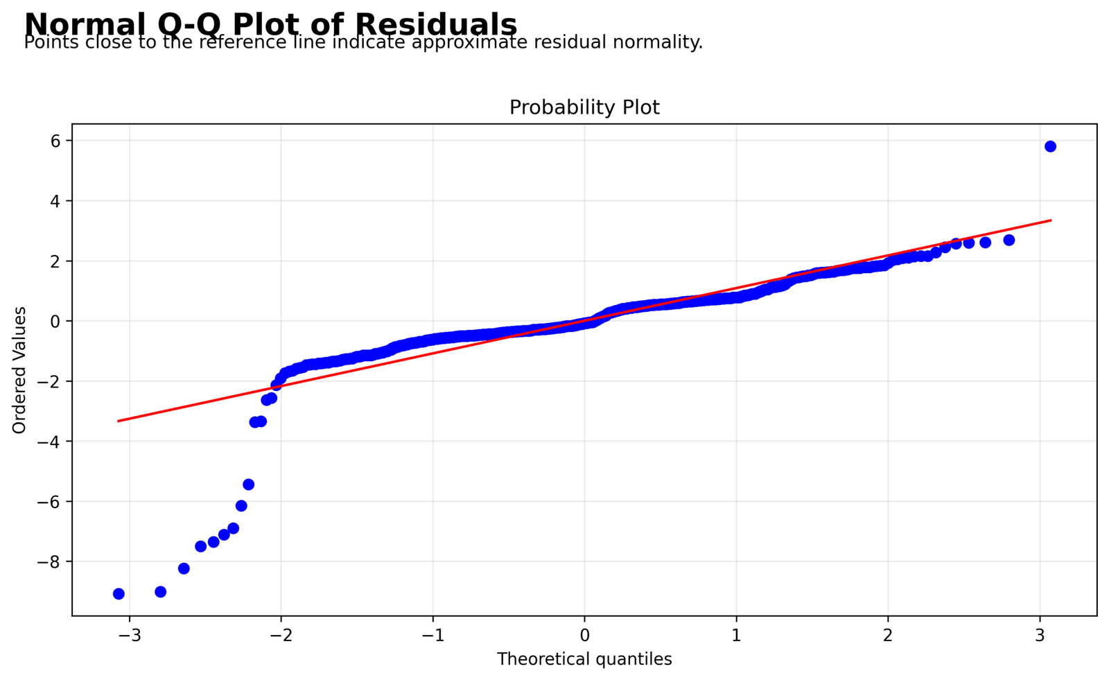
The central quantiles follow the reference more closely than the tails. The lower tail departs because of several unusually large negative residuals.
18 standardized residuals exceed ±2, and 10 exceed ±3 in absolute value. The most extreme standardized residual is approximately −7.236.
Exact normality is not supported in the extreme tails. With 649 observations, the omnibus model signal remains very strong, but conventional inference should still acknowledge unusual cases.
The Q-Q plot complements Q-Q Plot Normality Check guidance and identifies where finite-sample reference assumptions are least credible.
Python Chart 6: Coefficients with 95% Confidence Intervals
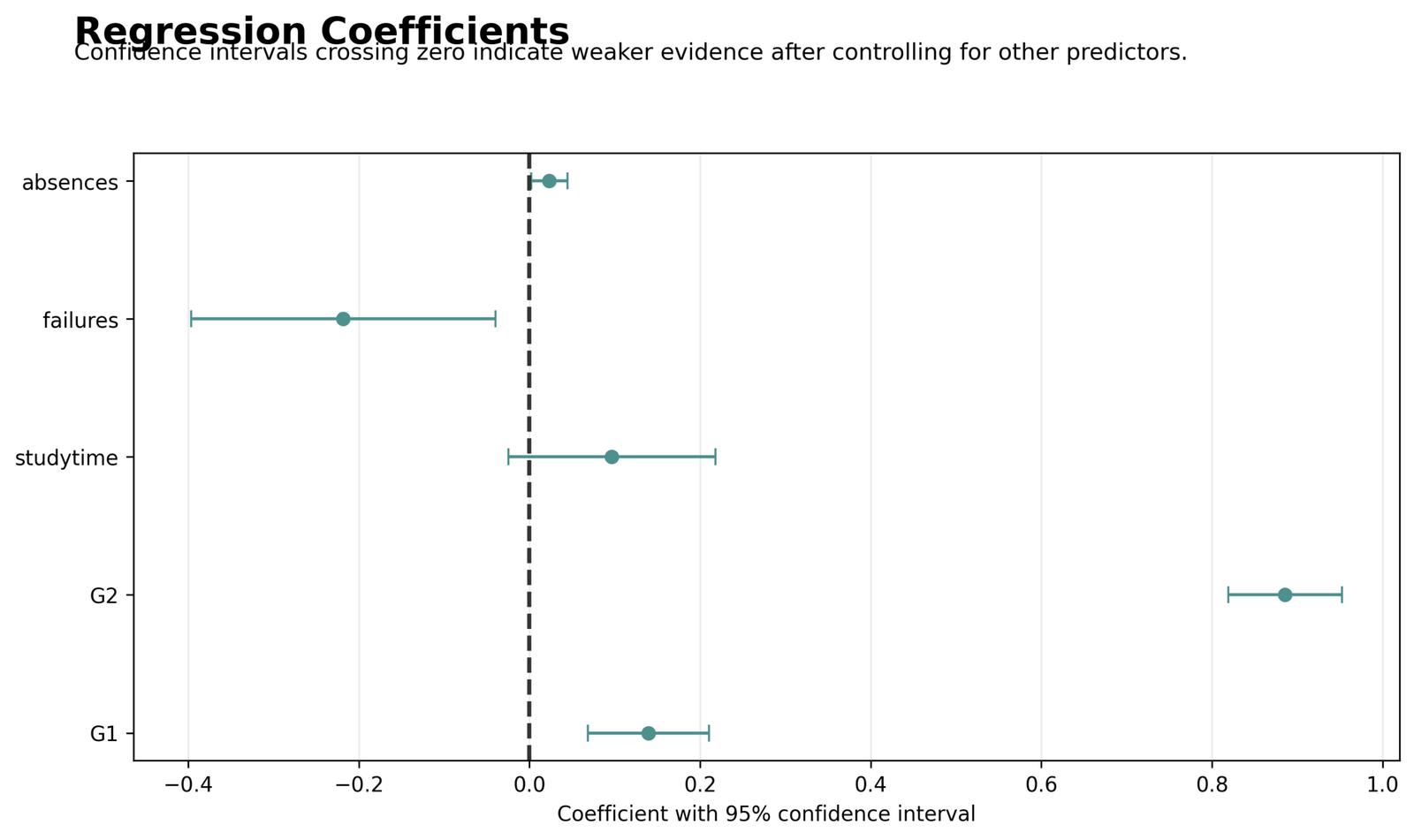
G2 is the dominant positive coefficient. G1 is also positive. Failures is negative. Absences is small but positive. The studytime interval crosses zero.
G1 B = 0.13946, G2 B = 0.88571, studytime B = 0.09670, failures B = −0.21829, and absences B = 0.02337.
The Regression ANOVA Table establishes collective significance, while this chart shows which conditional slopes provide individual evidence. G1, G2, failures, and absences exclude zero at the 95% level.
Omnibus significance and coefficient significance answer different questions. Interpret estimates with Confidence Interval and P-Value guidance.
Python Chart 7: R-Squared and Error Summary
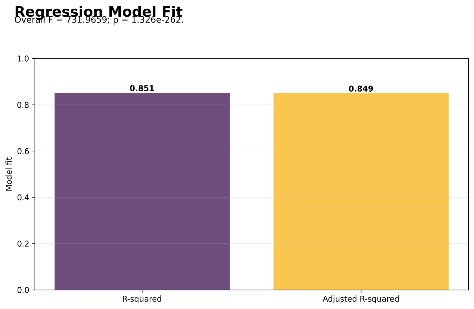
R² and adjusted R² are very close, showing that the strong fit is not an artifact of adding five predictors to a small sample.
R² = 0.850563, adjusted R² = 0.849401, and RMSE = 1.253722.
About 85.06% of sample variation is explained, but typical prediction error remains around 1.25 grade points. Relative fit and original-unit error describe different aspects of performance.
Use the dedicated Adjusted R-Squared guide when comparing models with different predictor counts.
Python Chart 8: Residual Sequence
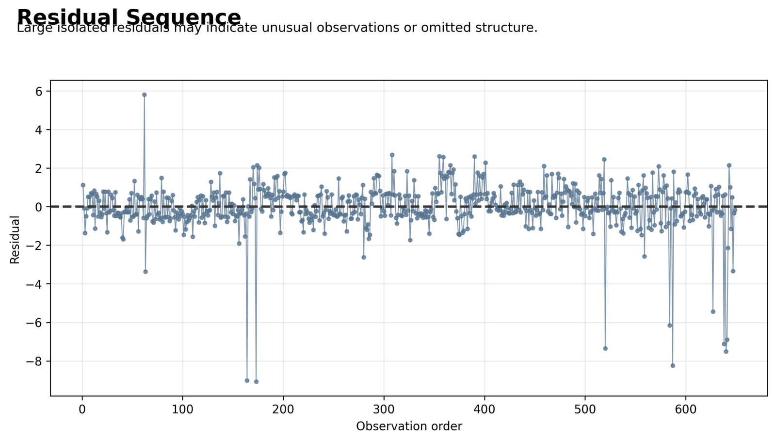
The sequence fluctuates around zero with several isolated extreme negative errors and one large positive error. No single long monotonic drift dominates the full series.
The Durbin-Watson value computed from the supplied residual sequence is approximately 1.857. The largest negative residual is −9.0716, and the largest positive residual is 5.8068.
The ordering evidence does not indicate severe first-order dependence, but record order may not represent a meaningful time sequence. Independence must come from the study design as well as the graph.
Use Durbin-Watson Test only when the observation order has a legitimate temporal or sequential interpretation.
R Charts and Explanations
The R visuals reproduce the supplied Regression ANOVA Table evidence with two chart pairs. A single cross-software conclusion is sufficient: Python and R agree on the sums of squares, fitted-value pattern, and residual concentration.
R Sum-of-Squares Partition
The R bars reproduce SSR = 5752.5873 and SSE = 1010.6793. Their sum returns SST = 6763.2666, and the explained share returns R² = 0.850563.
R Observed Versus Fitted Values
The main point cloud follows the agreement line, while the largest deviations occur for unusual low outcomes. This pattern explains the high R² and the non-negligible residual tail at the same time.
R Residuals Versus Fitted Values
Residuals remain broadly centered around zero. The integer outcome creates diagonal bands, and a small set of extreme negative residuals accounts for much of the tail behavior.
R Residual Histogram
The distribution is concentrated near zero but has a longer negative tail. The shape agrees with the Python histogram and the large squared residuals identified in the case review.
Regression Coefficient Interpretation
| Term | B | SE | t | p | 95% CI | Interpretation |
|---|---|---|---|---|---|---|
| Intercept | −0.155190 | 0.258626 | −0.6001 | .5487 | −0.663043 to 0.352663 | Predicted G3 when every predictor equals zero; not substantively central here |
| G1 | 0.139457 | 0.036227 | 3.8495 | .00013 | 0.068319 to 0.210596 | One additional G1 point is associated with 0.139 higher G3, holding other predictors constant |
| G2 | 0.885709 | 0.033927 | 26.1066 | <.001 | 0.819088 to 0.952329 | Dominant positive conditional predictor of G3 |
| studytime | 0.096699 | 0.061810 | 1.5645 | .1182 | −0.024674 to 0.218073 | Positive point estimate, but the interval includes zero |
| failures | −0.218290 | 0.090861 | −2.4025 | .0166 | −0.396711 to −0.039870 | Each additional failure is associated with 0.218 lower G3 after adjustment |
| absences | 0.023367 | 0.010794 | 2.1648 | .0308 | 0.002171 to 0.044562 | Small positive adjusted association that should not be interpreted causally |
Fitted Regression Equation
G2 provides the largest conditional contribution because a one-point G2 difference corresponds to nearly 0.886 predicted G3 points after the remaining predictors are controlled. G1 adds a smaller independent positive contribution.
The negative failures coefficient is consistent with lower final grades among students with more previous failures. The small positive absences coefficient should be interpreted cautiously because it is conditional on prior grades and failures and may reflect suppression, coding structure, or omitted variables rather than a beneficial absence effect.
Studytime is not statistically significant at α = .05. That does not prove a population effect of exactly zero. Its confidence interval includes both a small negative effect and a moderate positive effect.
Predictions and Residual Contributions
Mean-Profile Prediction
Substituting the sample means into the fitted equation gives:
With an intercept, the average fitted value equals the average observed outcome. This is another useful audit of an ordinary least squares model.
How Individual Cases Build SSE
Every residual equals observed G3 minus fitted G3. Squaring each residual and summing all 649 values gives SSE = 1010.6792762223604. The largest errors contribute disproportionately because a residual twice as large creates four times as much squared error.
| Case | Observed G3 | Fitted G3 | Residual | Standardized residual | Squared residual |
|---|---|---|---|---|---|
| 173 | 1 | 10.0716 | −9.0716 | −7.2357 | 82.2935 |
| 164 | 0 | 9.0103 | −9.0103 | −7.1869 | 81.1862 |
| 587 | 0 | 8.2395 | −8.2395 | −6.5721 | 67.8900 |
| 640 | 0 | 7.5062 | −7.5062 | −5.9871 | 56.3427 |
| 520 | 0 | 7.3538 | −7.3538 | −5.8656 | 54.0788 |
| 62 | 16 | 10.1932 | 5.8068 | 4.6317 | 33.7193 |
The six cases shown above contribute more than 375 squared-error units combined. They illustrate why residual diagnostics matter even when R² exceeds .85.
The complete 649-row prediction and residual register remains available in the worked Excel workbook rather than being reproduced as an unreadable public table.
Regression ANOVA Table Assumptions and Diagnostics
Model evidence
- R² = 0.850563
- Adjusted R² = 0.849401
- RMSE = 1.253722
- F(5, 643) = 731.9659
- p < .001
Diagnostic cautions
- Long negative residual tail
- 10 standardized residuals beyond ±3
- Potential influence from extreme low outcomes
- Conditional interpretation of absences
- Need to verify linearity and variance
Linearity
The equation assumes that each predictor has an additive linear relationship with expected G3 after the others are controlled. Residual-versus-fitted plots should not contain a remaining systematic curve. If curvature is visible, transformations, polynomial terms, or another mean function may be needed.
Homoskedasticity
The classical F test uses one pooled error variance represented by MSE = 1.571818470019223. If residual spread changes substantially across fitted values, heteroskedasticity-robust inference may be preferable. Use the residual plot with Breusch-Pagan Test and White Test as supporting checks.
Residual Normality
The histogram and Q-Q plot show a concentrated center with tail departures. Normality is not required for unbiased OLS coefficients under the standard exogeneity assumptions, but it affects exact small-sample t and F reference distributions. The large sample reduces sensitivity, although the extreme cases remain important.
Independence
Independence comes primarily from study design. The residual sequence has an approximate Durbin-Watson value of 1.857, but this statistic is meaningful only when row order represents time or another genuine sequence. Clustered students or repeated measurements would require a different covariance model.
Multicollinearity
G1 and G2 are related prior-grade measures. The overall F test can remain highly significant even when individual coefficients are affected by overlap. Review Variance Inflation Factor and Tolerance Statistic before interpreting coefficient magnitudes as independent importance rankings.
Influence
Cases 173, 164, 587, 640, and 520 have very large negative residuals. Residual size alone does not measure leverage, so use Cook’s Distance, Influence Diagnostics, and Studentized Residuals to determine whether those cases materially change the fitted equation.
Outcome Construction and Availability
G1 and G2 are prior grades closely related to G3. They explain much of the outcome, but analysts should consider whether both predictors are available at the time a real decision would be made. Strong retrospective fit is not identical to early forecasting usefulness.
Regression ANOVA Table in Python, R, SPSS and Excel
Python
Python can fit the OLS equation with statsmodels and reconstruct every Regression ANOVA Table value from fitted and residual arrays.
- Fit G3 on five predictors
- Calculate SSR, SSE, and SST directly
- Verify F and R² independently
- Save fitted values and residual diagnostics
R
R uses lm() for estimation and anova() for the model table. Direct residual and fitted-value calculations can verify the software output.
summary(model)for coefficients and R²anova(model)for the F tablefitted()andresiduals()for audit calculations- Diagnostic plots for assumptions
SPSS
SPSS REGRESSION produces Model Summary, ANOVA, and Coefficients tables. Save predicted values and residuals so the ANOVA rows can be checked against case-level output.
- Dependent: G3
- Predictors: G1, G2, studytime, failures, absences
- Request ANOVA, coefficients, and confidence intervals
- Save predicted and residual values
Excel
Excel can reconstruct the Regression ANOVA Table with fitted values, residuals, squared residuals, and sums around the outcome mean. The Analysis ToolPak also provides a standard regression output.
- Calculate ŷ from the fitted equation
- Calculate residual and squared residual
- Sum explained and residual components
- Verify mean squares and F with formulas
Code: Expand Only the Software You Need
Python Regression ANOVA Table code
import numpy as np
import pandas as pd
import statsmodels.api as sm
from scipy import stats

df = pd.read_csv("dataset.csv")
variables = ["G3", "G1", "G2", "studytime", "failures", "absences"]
work = df[variables].dropna().copy()

y = work["G3"].astype(float)
X = sm.add_constant(
    work[["G1", "G2", "studytime", "failures", "absences"]].astype(float)
)

model = sm.OLS(y, X).fit()
fitted = model.fittedvalues
residual = model.resid

y_mean = y.mean()
ss_total = float(((y - y_mean) ** 2).sum())
ss_error = float((residual ** 2).sum())
ss_regression = float(((fitted - y_mean) ** 2).sum())

df_regression = int(model.df_model)
df_error = int(model.df_resid)
ms_regression = ss_regression / df_regression
ms_error = ss_error / df_error
f_value = ms_regression / ms_error
p_value = stats.f.sf(f_value, df_regression, df_error)

print("SSR:", ss_regression)
print("SSE:", ss_error)
print("SST:", ss_total)
print("MSR:", ms_regression)
print("MSE:", ms_error)
print("F:", f_value)
print("p:", p_value)
print("R-squared:", ss_regression / ss_total)
print(model.summary())
R Regression ANOVA Table code
df <- read.csv("dataset.csv")

work <- na.omit(
  df[c("G3", "G1", "G2", "studytime", "failures", "absences")]
)

model <- lm(
  G3 ~ G1 + G2 + studytime + failures + absences,
  data = work
)

y <- work$G3
fitted_values <- fitted(model)
residual_values <- residuals(model)
y_mean <- mean(y)

ss_total <- sum((y - y_mean)^2)
ss_error <- sum(residual_values^2)
ss_regression <- sum((fitted_values - y_mean)^2)

df_regression <- length(coef(model)) - 1
df_error <- df.residual(model)

ms_regression <- ss_regression / df_regression
ms_error <- ss_error / df_error
f_value <- ms_regression / ms_error
p_value <- pf(f_value, df_regression, df_error, lower.tail = FALSE)

anova(model)
summary(model)

c(
  SSR = ss_regression,
  SSE = ss_error,
  SST = ss_total,
  MSR = ms_regression,
  MSE = ms_error,
  F = f_value,
  p = p_value
)
SPSS Regression ANOVA Table syntax
REGRESSION
 /DEPENDENT G3
 /METHOD=ENTER G1 G2 studytime failures absences
 /STATISTICS COEFF OUTS R ANOVA CI(95) COLLIN TOL
 /SAVE PRED(PRED_G3)
       RESID(RESID_G3)
       SRESID(SRESID_G3)
       COOK(COOK_D).

OUTPUT SAVE OUTFILE=
'D:\DATA ANALYSIS\H Regression Tests and Models\Regression ANOVA Table\SPSS_Output\spv\Regression-ANOVA-Table-SPSS-Output.spv'.

OUTPUT EXPORT
 /CONTENTS EXPORT=ALL LAYERS=PRINTSETTING MODELVIEWS=PRINTSETTING
 /PDF DOCUMENTFILE=
'D:\DATA ANALYSIS\H Regression Tests and Models\Regression ANOVA Table\SPSS_Output\pdf\Regression-ANOVA-Table-SPSS-Output.pdf'.
Excel Regression ANOVA Table formulas
Predicted G3:
=Intercept
 + G1*B_G1
 + G2*B_G2
 + Studytime*B_Studytime
 + Failures*B_Failures
 + Absences*B_Absences

Residual:
=Observed_G3-Predicted_G3

Squared residual:
=Residual^2

SSE:
=SUM(Squared_Residual_Range)

SST contribution:
=(Observed_G3-AVERAGE(Observed_G3_Range))^2

SSR contribution:
=(Predicted_G3-AVERAGE(Observed_G3_Range))^2

MSR:
=SSR/5

MSE:
=SSE/643

F:
=MSR/MSE

F p-value:
=F.DIST.RT(F_Value,5,643)

R-squared:
=SSR/SST

RMSE:
=SQRT(MSE)
Advanced Regression ANOVA Table Topics
Regression ANOVA Table for Beginners
A Regression ANOVA Table is a three-row summary showing variation explained by a regression, variation left in residuals, and total outcome variation.
Regression ANOVA Table Formula
The core identity is SST = SSR + SSE. Mean squares divide SSR and SSE by their degrees of freedom, and F = MSR/MSE.
Regression ANOVA Table Degrees of Freedom
With n observations and p slopes, regression df = p, error df = n − p − 1, and total df = n − 1.
Regression Sum of Squares
Regression sum of squares measures how much fitted values vary around the outcome mean. It represents improvement over an intercept-only model.
Residual Sum of Squares
Residual sum of squares is the sum of squared observed-minus-fitted errors. It is also called error sum of squares.
Total Sum of Squares
Total sum of squares measures outcome variation around the sample mean before predictors are used.
Mean Square Regression
MSR is SSR divided by regression degrees of freedom. It is the average explained square per model degree of freedom.
Mean Square Error
MSE is SSE divided by residual degrees of freedom. Under the classical model, it estimates residual variance.
Regression F Statistic
The F statistic is MSR/MSE and is interpreted using the F Distribution with numerator and denominator degrees of freedom.
Regression ANOVA Table P-Value
The p-value is the upper-tail probability of an F value at least as large under the collective null. See P-Value for reporting guidance.
Regression ANOVA Table and R-Squared
R² equals SSR/SST and also equals 1 − SSE/SST. The table therefore reconstructs R² directly.
Adjusted R-Squared
Adjusted R-Squared penalizes predictor count and is useful when comparing models with different numbers of slopes.
Regression ANOVA Table Versus Coefficients
The ANOVA row tests all slopes together. Coefficient rows test individual conditional slopes and provide direction and magnitude.
Regression ANOVA Table Versus One-Way ANOVA
Both are linear models using sums of squares. One-way ANOVA expresses predictors as groups; regression can include continuous predictors.
Type I Sum of Squares
Type I Sum of Squares measures sequential contributions in the order predictors enter the model.
Type II Sum of Squares
Type II Sum of Squares tests each main effect after the other main effects, usually without adjusting a main effect for interactions containing it.
Type III Sum of Squares
Type III Sum of Squares tests each term after all other terms and depends on coding choices in unbalanced designs.
Hierarchical Regression ANOVA
Nested block comparisons use changes in SSR and changes in degrees of freedom to test whether added predictors improve the model.
Partial F Test
A partial F test compares a reduced model with a full nested model. It is different from the full-model test against the intercept-only baseline.
Regression ANOVA Table Assumptions
The arithmetic decomposition always holds with an intercept, but conventional inference depends on the conditions discussed in ANOVA Assumptions.
Heteroskedasticity
Unequal residual variance can make conventional standard errors unreliable. Use Breusch-Pagan Test or White Test as supporting checks.
Residual Normality
Normality affects exact finite-sample inference. Use a histogram and Q-Q Plot Normality Check rather than a single test alone.
Influential Cases
Large residuals and high leverage can alter coefficients and SSE. Review Cook’s Distance and Influence Diagnostics.
Regression ANOVA Table in Excel
Excel can reconstruct every row from observed outcomes, fitted values, residuals, and degrees of freedom.
Regression ANOVA Table in SPSS
SPSS displays Model Summary, ANOVA, and Coefficients tables. Saved predictions and residuals allow independent verification.
Reporting a Regression ANOVA Table
Report F with both degrees of freedom, p-value, R², adjusted R², RMSE or residual standard error, predictors, sample size, and relevant diagnostics.
APA-Style Reporting
The Regression ANOVA Table showed SSR = 5752.59, SSE = 1010.68, SST = 6763.27, MSR = 1150.52, and MSE = 1.572. RMSE was 1.254 G3 points.
G1 was positively associated with G3, B = 0.139, SE = 0.036, t = 3.85, p < .001, 95% CI [0.068, 0.211]. G2 was the strongest positive predictor, B = 0.886, SE = 0.034, t = 26.11, p < .001, 95% CI [0.819, 0.952]. Failures was negatively associated with G3, B = −0.218, SE = 0.091, t = −2.40, p = .017, 95% CI [−0.397, −0.040].
Absences had a small positive adjusted coefficient, B = 0.023, SE = 0.011, t = 2.16, p = .031, 95% CI [0.002, 0.045], whereas studytime was not statistically significant, B = 0.097, SE = 0.062, t = 1.56, p = .118.
Residual diagnostics showed a concentrated central error distribution with several large negative residuals, so unusual cases should be considered when interpreting the conventional inference.
Publication Checklist
Include
- Outcome and predictor names
- Complete-case sample size
- Regression, error, and total sums of squares
- All degrees of freedom
- MSR, MSE, F, and p
- R² and adjusted R²
- RMSE or residual standard error
- Coefficient estimates and confidence intervals
- Residual and influence diagnostics
- Software and reproducible specification
Avoid
- Calling SSR a causal contribution
- Claiming every predictor is significant
- Reporting F without both degrees of freedom
- Confusing MSE with RMSE
- Using R² as a prediction-error unit
- Ignoring influential observations
- Omitting the intercept convention
- Mixing sums-of-squares types without explanation
- Relying on p-values without effect estimates
- Presenting the 649-row residual register in the public article
Responsible reporting should also distinguish Effect Size, Statistical Power, and Type I and Type II Error from the model’s omnibus p-value.
Downloads
Regression ANOVA Table R ReportR model output and four verification charts
Regression ANOVA Table SPSS OutputSPSS Model Summary, ANOVA, Coefficients, and diagnostic output
Regression ANOVA Table Worked ExcelFormulas, model results, and complete prediction/residual register
Frequently Asked Questions
What is a Regression ANOVA Table?
It is the three-row sums-of-squares table for an ordinary least squares model, separating explained, residual, and total outcome variation.
What are the three rows in a Regression ANOVA Table?
The rows are Regression or Model, Residual or Error, and Total.
What is the Regression ANOVA Table formula?
The core identity is SST = SSR + SSE. Mean squares are MSR = SSR/dfRegression and MSE = SSE/dfError, and F = MSR/MSE.
How are Regression ANOVA Table degrees of freedom calculated?
With n observations and p slopes, regression df = p, error df = n − p − 1, and total df = n − 1.
How is F = 731.9659 obtained?
Divide MSR = 1150.5175 by MSE = 1.571818. The result is 731.9659.
What does the Regression ANOVA Table p-value test?
It tests the collective null that all slope coefficients equal zero.
Does a significant Regression ANOVA Table mean every predictor is significant?
No. It means at least one slope contributes information. Individual coefficient tests determine which slopes have stronger evidence.
How does the Regression ANOVA Table relate to R-squared?
R² equals SSR/SST. Here, 5752.5873 divided by 6763.2666 equals 0.850563.
Is residual mean square the same as RMSE?
No. MSE is residual variance in squared outcome units. RMSE is the square root of MSE and is reported in outcome units.
Why is total df 648?
There are 649 observations, so total df = n − 1 = 648.
Why is error df 643?
Five slopes and one intercept are estimated, so error df = 649 − 5 − 1 = 643.
What is the difference between a Regression ANOVA Table and coefficient table?
The ANOVA table tests the predictor set collectively. The coefficient table reports direction, size, and uncertainty for individual slopes.
Can a Regression ANOVA Table detect heteroskedasticity?
No. Use residual-versus-fitted plots and supporting variance diagnostics.
What do Type I, Type II, and Type III sums of squares mean?
They are different ways to assign partial sums of squares in models with multiple terms, especially unbalanced or interaction designs.
How do I create a Regression ANOVA Table in Excel?
Calculate fitted values, residuals, squared residuals, SST, SSR, SSE, degrees of freedom, mean squares, F, and the right-tail F probability.
How should a Regression ANOVA Table be reported?
Report F with numerator and denominator df, p, R², adjusted R², sample size, predictor set, original-unit error, coefficient evidence, and relevant diagnostics.
Regression ANOVA Table Conclusion
The Regression ANOVA Table for this five-predictor model is mathematically complete and internally consistent. Regression and error sums of squares add to total variation, their degrees of freedom add to total degrees of freedom, and their mean-square ratio reproduces the reported F statistic.
The model explains approximately 85.06% of G3 variation, F(5, 643) = 731.97, p < .001, with RMSE of approximately 1.254 grade points. G2 is the dominant positive conditional predictor, followed by a smaller positive G1 coefficient. Failures is negative, absences is small and positive after adjustment, and studytime remains uncertain.
The model-wide conclusion is strong, but it is not the whole analysis. Several extreme residuals contribute heavily to SSE, the lower residual tail departs from normality, and individual prediction errors remain visible despite the high R².

