
Weighted Least Squares Regression: Formula, Weights, Breusch-Pagan Test and Interpretation
Weighted Least Squares Regression estimates a linear conditional mean while giving greater influence to observations with lower estimated error variance. This worked guide predicts final grade G3 for 649 students, diagnoses non-constant OLS variance, constructs bounded inverse-variance weights, and compares OLS and WLS coefficients, fit and diagnostics in Python, R, SPSS and Excel.
Weighted Least Squares Regression Model Overview
Weighted Least Squares Regression is used when a linear conditional mean remains appropriate but the residual variance is not constant. Ordinary least squares gives every record equal influence. WLS instead minimizes a squared-error objective in which each residual is multiplied by a positive observation-specific precision weight.
The outcome is G3. Numeric predictors are G1, G2, studytime, failures, absences and age. Categorical terms are school, sex and address, with GP, female and rural as references. The same mean formula and the same 649 observations are used in OLS and WLS so coefficient differences reflect the weighting rule rather than a changing sample.
What problem does WLS solve?
OLS coefficient estimates can remain unbiased under heteroscedasticity when exogeneity holds, but conventional standard errors are inefficient or incorrect and equal weighting may not use the most precise observations effectively. WLS seeks greater efficiency when relative conditional variances can be modeled credibly.
What the weights mean
A weight is proportional to inverse estimated error variance. A value above one indicates modeled precision above the sample average; a value below one indicates higher modeled noise. The weight does not measure a student’s substantive importance, probability, frequency or survey representation.
How the two-stage model is constructed
First, the full OLS mean equation is fitted. Second, log residual squared plus a stabilizing constant is modeled from the OLS fitted value and its absolute value. The predicted log variances are exponentiated, inverted, clipped at the first and ninety-ninth percentiles and scaled to mean one. Finally, the identical mean equation is refitted with those weights.
When to use WLS
- The outcome is continuous.
- The conditional mean is linear in the selected predictors.
- Residual variance changes systematically across observations.
- Relative precision can be known or estimated plausibly.
- The resulting weights are positive, stable and auditable.
When not to use WLS
- The mean equation is misspecified through omitted curvature or interactions.
- Dependence or clustering is the main problem.
- Weights are arbitrary or chosen to obtain preferred results.
- The intended weights are actually survey, frequency, propensity or robust influence weights.
- A few extreme weights dominate the fit without scientific justification.
Related methods
Ordinary Least Squares Regression is the equal-weight baseline. Robust Regression limits influence from large residuals rather than representing inverse precision. Generalized Least Squares Regression extends the idea to broader covariance structures, including correlated errors.
Advantages
- Can improve efficiency when relative variances are modeled well.
- Makes the variance problem explicit rather than hiding it in one robust standard error.
- Allows direct inspection of the weight distribution.
- Retains the original linear coefficient interpretation.
Limitations
- Estimated weights introduce a second modeling stage.
- A significant heteroscedasticity test does not prove one variance function is correct.
- WLS does not repair omitted variables, dependence, nonlinearity or causal confounding.
- Weighted fit statistics require careful definition and cannot always be compared directly with OLS values.
Current worked scenario
The OLS Breusch-Pagan LM statistic is 34.014662 with p = 0.000088795, and the F version is 3.926990 with p = 0.000070438. Final weights average one and range from 0.5477 to 1.5136. WLS adjusted R² is 0.862019 and weighted RMSE is 1.148225.
Quick Answer
Why weighting is justified
- Breusch-Pagan LM p = 0.000088795.
- Breusch-Pagan F p = 0.000070438.
- OLS residual spread changes across fitted values.
- The estimated variance stage produces positive moderate weights.
What weighting changes
- Adjusted R² rises from 0.850141 to 0.862019.
- Weighted RMSE is 1.148225.
- G2 changes from 0.8794 to 0.8561.
- Failures changes from -0.2266 to -0.2766.
The ordinary RMSE is 1.240967 for OLS and 1.242420 for WLS. That is not a contradiction. OLS minimizes unweighted squared error, whereas WLS minimizes a precision-weighted squared error whose RMSE is 1.148225.
Table of Contents
- Model Overview
- Quick Answer
- Why WLS Is Needed
- How WLS Works
- Variables and Coding
- Verified Results
- Python Chart Stories
- R Chart Pairs
- Coefficient Interpretation
- Predictions and Meaning
- Assumptions and Diagnostics
- Python, R, SPSS and Excel
- Code and Formulas
- Advanced Topics
- APA-Style Reporting
- Publication Checklist
- Downloads
- Related Guides
- Frequently Asked Questions
- Conclusion
Why This Analysis Needs Weighted Least Squares Regression
The OLS baseline assumes that residuals have equal conditional variance. In the worked data, residual spread changes with fitted grade. If all observations are treated as equally precise, noisier regions influence the equation as strongly as more stable regions.
The significant Breusch-Pagan Test supports investigating unequal variance. It does not prove that the chosen auxiliary model is uniquely correct. The variance curve and clipping rule remain assumptions that require sensitivity checks.
WLS changes observation influence without changing the outcome or predictor values. It is therefore preferable to manually altering outcomes or deleting noisy cases solely to improve fit.
How Weighted Least Squares Regression Works
Weighted objective
W is a diagonal matrix containing one positive weight for each observation. When weights are proportional to inverse conditional variance, high-precision observations contribute more to the coefficient solution.
Three-stage workflow
Save fitted values and residuals.
Model log residual squared and invert predictions.
Use clipped, mean-scaled positive weights.
Auxiliary variance equation
The stabilizing constant is the larger of residual variance × 10⁻⁶ and 10⁻⁸. Exponentiation produces positive estimated variance. Inversion converts variance to precision.
Clipping and scaling
Raw weights are clipped at the first and ninety-ninth percentiles and then divided by their mean. Clipping limits unstable tail influence, while scaling makes one the average precision level.
Scaling all weights by one common positive constant does not change the fitted point coefficients.
Variables Used, Coding and Weight Meaning
| Role | Term | Coding or unit | Weighted interpretation |
|---|---|---|---|
| Outcome | G3 | Final grade | Continuous weighted mean target |
| Numeric predictor | G1 | First-period grade | Expected G3 change for one-point G1 difference |
| Numeric predictor | G2 | Second-period grade | Expected G3 change for one-point G2 difference |
| Numeric predictor | studytime | Ordinal weekly study-time code | One-category difference under linear coding |
| Numeric predictor | failures | Past class-failure count/code | Expected change for one additional failure unit |
| Numeric predictor | absences | School absence count | Expected G3 change per additional absence |
| Numeric predictor | age | Age in years | Expected G3 change per year |
| Indicator | school_MS | MS compared with GP | Reference category: GP |
| Indicator | sex_M | Male compared with female | Reference category: female |
| Indicator | address_U | Urban compared with rural | Reference category: rural |
The same formula is used in both models: G3 ~ G1 + G2 + studytime + failures + absences + age + school + sex + address. With nine predictor degrees of freedom and an intercept, residual degrees of freedom are 639.
Verified Weighted Least Squares Regression Results
Heteroscedasticity evidence
| Diagnostic | Statistic | p-value | Interpretation |
|---|---|---|---|
| Breusch-Pagan LM | 34.014662 | 0.000088795 | Reject constant OLS residual variance |
| Breusch-Pagan F | 3.926990 | 0.000070438 | Reject constant OLS residual variance |
| R manual fitted-value auxiliary test | 19.224437 | 0.0000116216 | Independent evidence of changing variance |
| OLS residual SD | 1.241925 | — | Raw baseline spread |
| WLS residual SD | 1.243375 | — | Raw spread is not the WLS optimization target |
OLS and WLS fit statistics
| Model | R² | Adjusted R² | Raw RMSE | Weighted RMSE | AIC | BIC | Objective |
|---|---|---|---|---|---|---|---|
| Ordinary least squares | 0.852222 | 0.850141 | 1.240967 | — | 2142.0090 | 2186.7633 | Equal observation influence |
| Weighted least squares | 0.863935 | 0.862019 | 1.242420 | 1.148225 | 2052.9054 | 2097.6597 | Scaled inverse estimated variance |
Coefficient comparison
| Term | OLS b | WLS b | WLS 95% CI | WLS p | Interpretation |
|---|---|---|---|---|---|
| Intercept | -0.2405 | -0.3660 | [-1.7755, 1.0434] | 0.6103 | Imprecise baseline |
| school_MS | -0.1665 | -0.1518 | [-0.3677, 0.0640] | 0.1677 | No clear weighted school contrast |
| sex_M | -0.2037 | -0.1680 | [-0.3569, 0.0210] | 0.0814 | OLS borderline result weakens |
| address_U | 0.0989 | 0.0759 | [-0.1353, 0.2871] | 0.4805 | No clear weighted address contrast |
| G1 | 0.1328 | 0.1419 | [0.0720, 0.2118] | 0.000075 | Positive and statistically supported |
| G2 | 0.8794 | 0.8561 | [0.7892, 0.9229] | 1.62 × 10−97 | Strongest positive slope |
| studytime | 0.0619 | 0.0506 | [-0.0636, 0.1648] | 0.3845 | Uncertain conditional effect |
| failures | -0.2266 | -0.2766 | [-0.4667, -0.0865] | 0.0044 | Negative and statistically supported |
| absences | 0.0177 | 0.0151 | [-0.0055, 0.0356] | 0.1501 | Small and uncertain |
| age | 0.0236 | 0.0436 | [-0.0365, 0.1238] | 0.2857 | Uncertain conditional effect |
Weight distribution and stabilization
| Quantity | Exact value | Meaning |
|---|---|---|
| Mean scaled weight | 1.0000 | Weights are normalized for interpretation |
| Minimum weight | 0.5477 | No observation receives near-zero influence |
| Maximum weight | 1.5136 | No observation dominates by orders of magnitude |
| Maximum/minimum ratio | 2.7635 | Moderate rather than extreme precision contrast |
| Clipping rule | 1st and 99th percentiles | Limits unstable inverse-variance tails |
The OLS overall F statistic is 409.4514 with p = 1.4403 × 10−258. The WLS overall F statistic is 450.8106 with p = 5.2574 × 10−270. Both models contain strong predictor signal; these tests do not validate the variance model by themselves.
Open the Main Reports
Use the PDFs to verify coefficients, weights, diagnostics and software-specific conventions.
Python Charts and Exact-Value Explanations
Each chart is explained using the full four-part pattern: what is visible, exact values, statistical meaning and the next verification step.
Python Chart 1: Outcome Distribution before Weight Construction
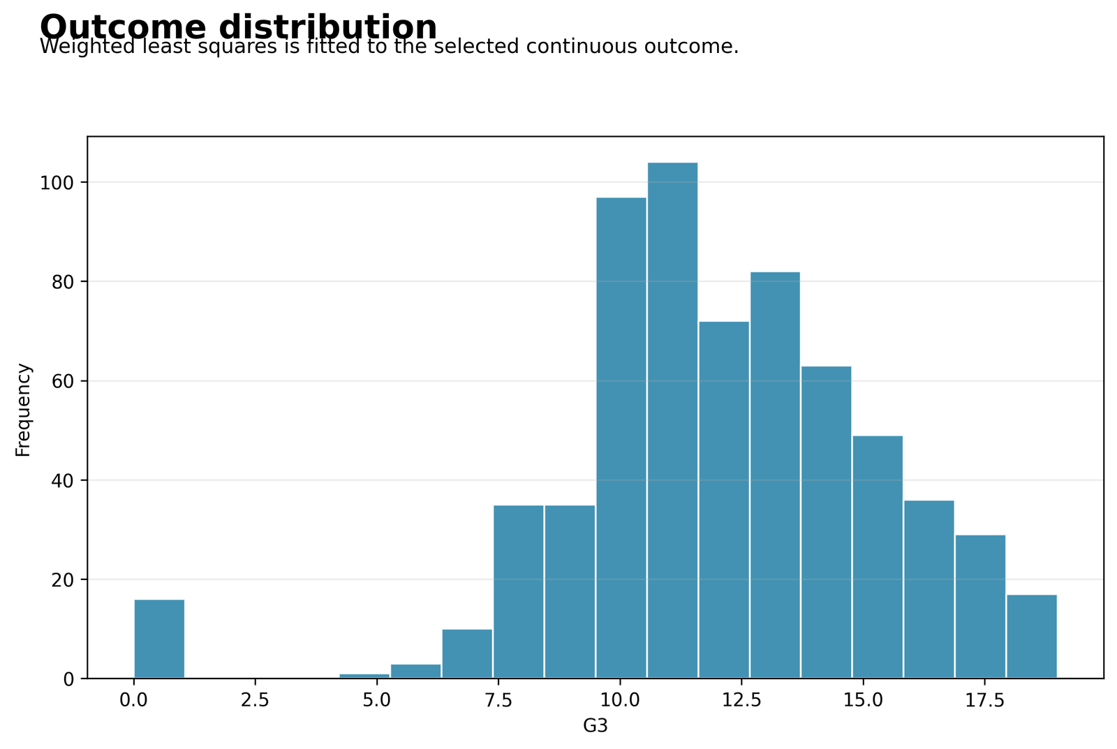
The histogram summarizes the final-grade outcome before the OLS baseline and variance model are fitted. It helps identify boundedness, concentration and tail behavior.
The analysis retains 649 observations. The same rows are used for OLS, the auxiliary variance model and the final weighted fit.
A marginally unusual outcome does not automatically receive a low or high weight. Precision weights depend on how variable G3 is conditionally at the fitted predictor profile.
Review Descriptive Statistics and Histogram Interpretation, then move to the OLS residual plot.
Python Chart 2: OLS Residuals versus Fitted Values
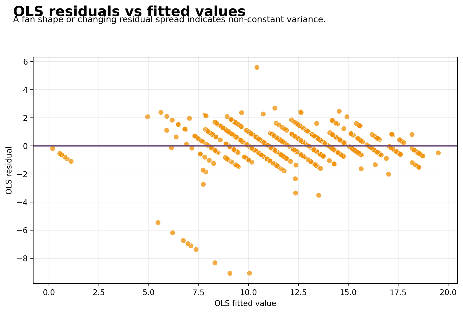
The vertical spread of residuals changes across fitted grades instead of remaining equally wide everywhere.
Breusch-Pagan LM = 34.014662, p = 0.000088795; F = 3.926990, p = 0.000070438.
The equal-variance assumption is not supported under the OLS model. This justifies investigating a feasible precision-weighting model, not automatically accepting any proposed weights.
Cross-check with Breusch-Pagan Test and White Test, then inspect the estimated variance curve.
Python Chart 3: Estimated Residual-Variance Pattern
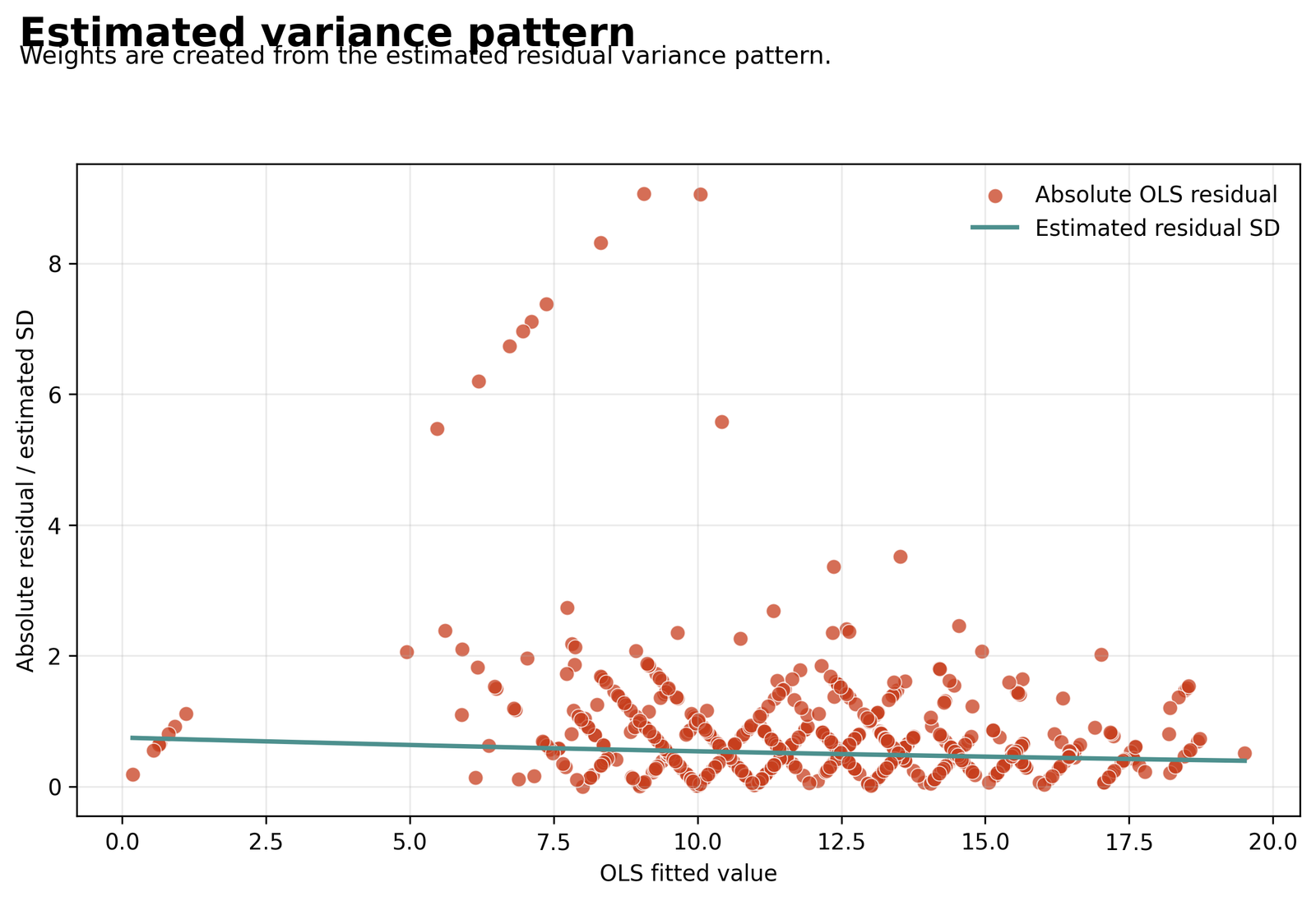
Absolute OLS residual behavior is summarized against fitted values, and the estimated standard-deviation pattern shows how precision changes across the fitted range.
The variance stage models log(e² + ε) from OLS fitted value and its absolute value. Final scaled weights range from 0.5477 to 1.5136.
High estimated variance produces a lower inverse-variance weight, while lower estimated variance produces a higher weight. The outcome is unchanged; only its contribution to squared loss changes.
Verify that predicted variances stay positive, inspect the weight range and report the epsilon, clipping and normalization rules.
Python Chart 4: Observed versus Weighted Fitted Values
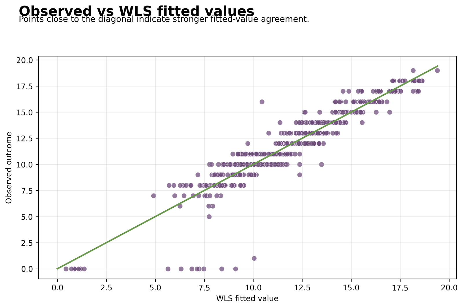
Points near the diagonal are predicted accurately under the weighted mean model, while vertical departures remain individual errors.
WLS R² = 0.863935, adjusted R² = 0.862019, raw RMSE = 1.242420 and weighted RMSE = 1.148225.
The weighted model performs well under its precision-weighted objective. Raw RMSE is not lower than OLS because OLS specifically minimizes unweighted squared error.
Use Adjusted R-Squared and state explicitly whether an error metric is weighted or unweighted.
Python Chart 5: OLS and WLS Coefficient Comparison
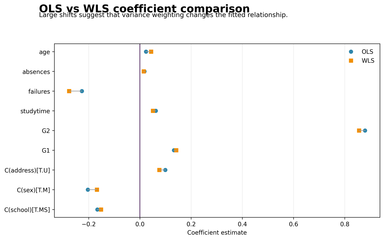
Most coefficient directions remain stable, but several estimates move enough to change substantive or threshold-based conclusions.
G2 changes from 0.8794 to 0.8561; failures changes from -0.2266 to -0.2766; sex_M p changes from 0.0493 under OLS to 0.0814 under WLS.
Weighting changes the influence of observations, so both estimates and standard errors can change. Do not select whichever coefficient or p-value is preferred.
Interpret the entire estimator and use Confidence Interval and P-Value together.
R Charts and Paired Explanations
The R section uses each supplied R image once. The duplicated residual image from the source article has been replaced by an exact-value analytical panel.
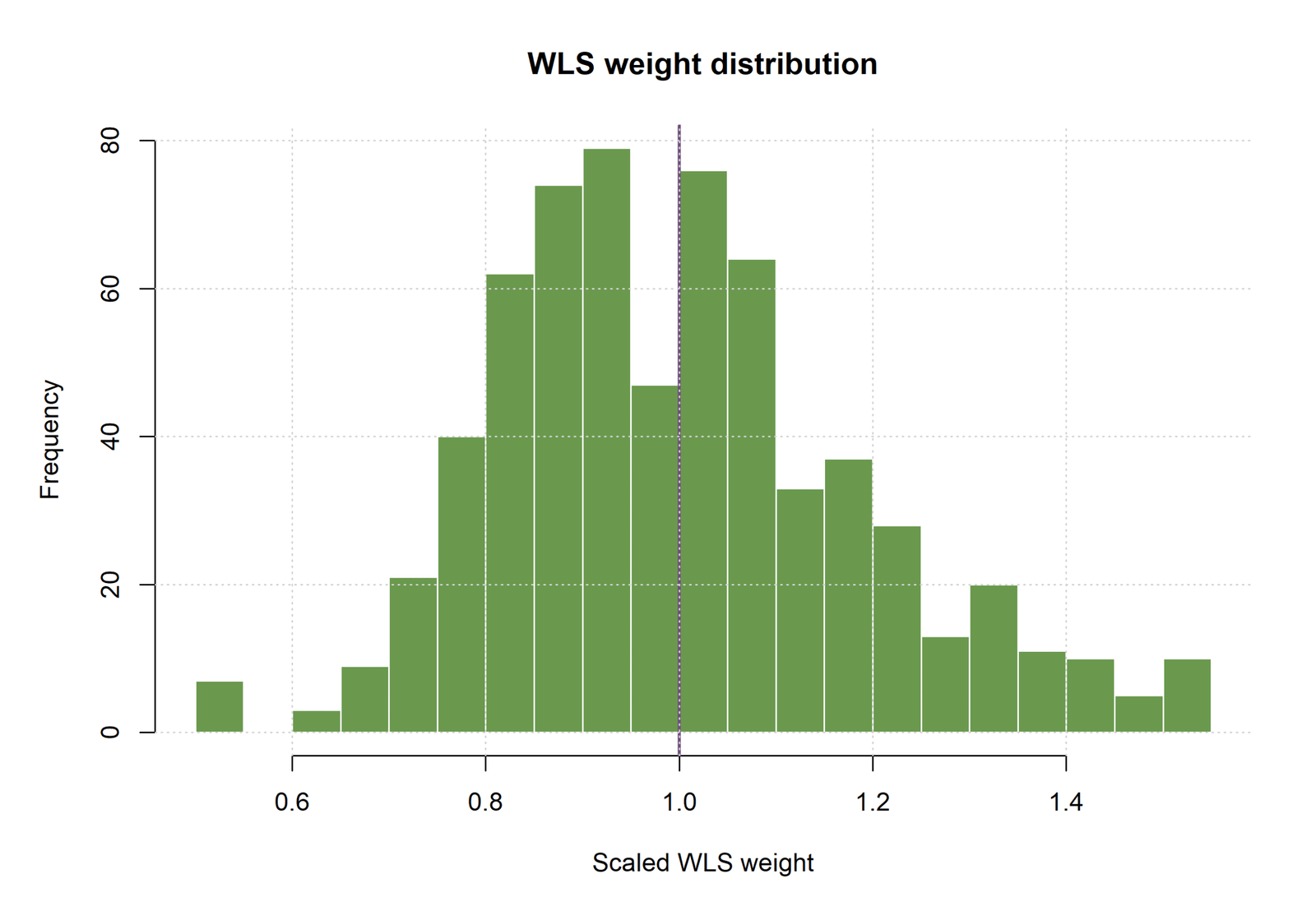
R Weight Distribution
The final weights are centered around one and stay within a moderate range. Values above one identify observations modeled as more precise; values below one identify noisier profiles.
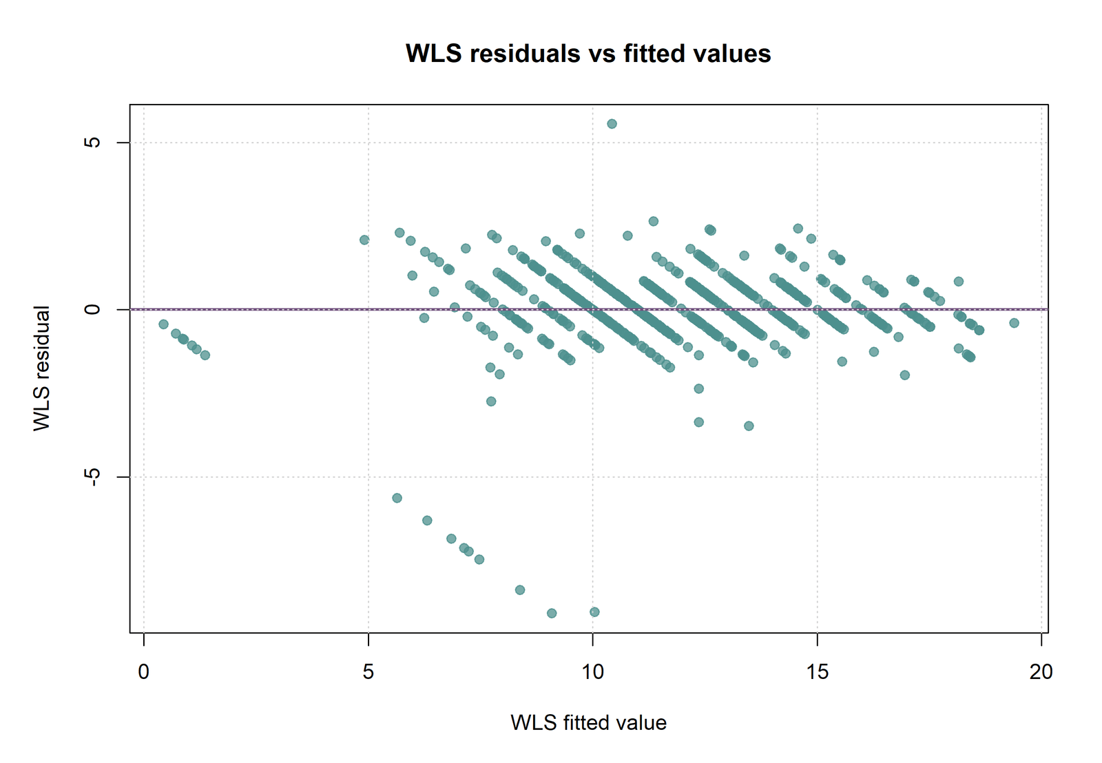
R Post-WLS Residual Diagnostic
The chart checks whether variance is more stable after applying the estimated precision pattern. A successful weighting model should reduce systematic spread without creating curvature.
R and Python cross-software summary
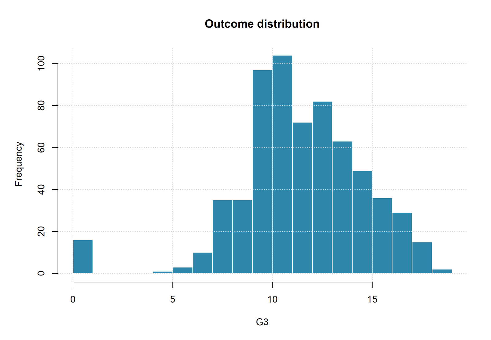
R Outcome Context
The marginal G3 distribution describes the response scale and tail behavior, but the weights are not calculated from outcome frequency alone.
Cross-Software Fit and Weight Agreement
R and Python agree on the 649-row mean equation, the weight range, the increase in adjusted R² and the weighted error objective.
Weighted Coefficient and Parameter Interpretation
G2
Holding all other terms fixed, one additional G2 point is associated with 0.8561 higher expected G3 under the weighted criterion. Its 95% interval [0.7892, 0.9229] is entirely positive.
G1
One additional G1 point is associated with 0.1419 higher expected G3, conditional on the remaining terms. The interval [0.0720, 0.2118] excludes zero.
Failures
One additional failure unit is associated with 0.2766 lower expected G3. The weighted magnitude is more negative than the OLS estimate.
Sex indicator
The WLS male coefficient is -0.1680 with p = 0.0814. The narrowly significant OLS result does not remain below the .05 threshold after weighting.
Other terms
School, address, studytime, absences and age have weighted intervals that include zero. This does not prove exact zero effects; it indicates that zero remains compatible with the fitted estimate and uncertainty.
Read Confidence Interval, Standard Error and Effect Size before reducing the table to significant versus nonsignificant labels.
Predictions, Effects and Model Meaning
New mean predictions use the weighted coefficient equation and the new predictor values. The training weights do not appear as another explanatory variable in that equation.
When prediction uncertainty or precision-weighted evaluation is required, the auxiliary variance model must also be applied to the new predictor profile. Using only the mean equation discards the precision component that motivated WLS.
What a weight does during estimation
For two observations with the same residual magnitude, a weight of 1.5 contributes three times as much weighted squared loss as a weight of 0.5. The higher-weight case is modeled as having one-third of the conditional variance of the lower-weight case.
What a weight does not mean
A weight does not multiply the predicted grade, represent the number of students, indicate treatment probability or certify data quality. It controls statistical influence in the stated weighted loss.
Weighted Least Squares Regression Assumptions and Diagnostics
Mean-model checks
- Linear conditional mean
- Appropriate predictor coding
- Independent observations
- No important omitted interactions or curvature
- No few observations dominate the weighted fit
Variance-model checks
- Predicted variances remain positive
- Weights are moderate and stable
- Clipping is disclosed
- Scaled residual spread improves
- Alternative variance specifications give compatible conclusions
Post-WLS residuals
Inspect raw residuals and residuals divided by estimated standard deviation. A good weighting rule should reduce systematic variance change without creating curvature or new influential points.
Normality
WLS does not force residuals to become normal. Use Q-Q Plot Normality Check, Shapiro-Wilk Test and Skewness and Kurtosis.
Influence and leverage
High precision weights can amplify leverage. Review Studentized Residuals, Cook’s Distance, Outlier Detection and Influence Diagnostics.
Predictor overlap
WLS does not remove multicollinearity. Review Variance Inflation Factor and Tolerance Statistic.
Weighted Least Squares Regression in Python, R, SPSS and Excel
Python
- Fit OLS with the full mean formula.
- Run Breusch-Pagan LM and F diagnostics.
- Estimate log residual variance.
- Clip, scale and pass weights to statsmodels WLS.
R
- Use the same sample and formula.
- Fit the auxiliary variance equation.
- Pass scaled inverse variances to lm(weights=).
- Export weights, coefficients and residual charts.
SPSS
- Fit the baseline and save residuals.
- Create or import the positive weight variable.
- Document the exact weight semantics.
- Archive syntax, SPV and PDF output.
Excel
- Demonstrate residual squares and variance estimates.
- Calculate inverse weights and mean scaling.
- Audit weighted cross-products.
- Keep demonstration coefficients separate from final estimates.
New users can review Correlation in Python, Correlation in R, Correlation in SPSS and Correlation in Excel before implementing the full workflow.
Code and Formula Panels
Python two-stage feasible WLS
ols = smf.ols(mean_formula, data=data).fit()
resid = np.asarray(ols.resid)
eps = max(np.nanvar(resid) * 1e-6, 1e-8)

variance_data = pd.DataFrame({
    "log_resid_sq": np.log(resid ** 2 + eps),
    "ols_fitted": np.asarray(ols.fittedvalues),
    "abs_ols_fitted": np.abs(np.asarray(ols.fittedvalues))
})

variance_fit = smf.ols(
    "log_resid_sq ~ ols_fitted + abs_ols_fitted",
    data=variance_data
).fit()

estimated_var = np.exp(variance_fit.predict(variance_data))
raw_weight = 1.0 / np.maximum(estimated_var, eps)
limits = np.percentile(raw_weight, [1, 99])
weight = np.clip(raw_weight, limits[0], limits[1])
weight = weight / weight.mean()

wls = smf.wls(mean_formula, data=data, weights=weight).fit()
R two-stage feasible WLS
ols <- lm(mean_formula, data = dat)
e <- resid(ols)
fit0 <- fitted(ols)
eps <- max(var(e) * 1e-6, 1e-8)

var_fit <- lm(log(e^2 + eps) ~ fit0 + abs(fit0))
estimated_var <- exp(predict(var_fit))
raw_w <- 1 / pmax(estimated_var, eps)

limits <- quantile(raw_w, c(.01, .99), na.rm = TRUE)
clipped_w <- pmin(pmax(raw_w, limits[1]), limits[2])
wls_weight <- clipped_w / mean(clipped_w)

wls <- lm(mean_formula, data = dat, weights = wls_weight)
SPSS weighted regression outline
* Import or compute a positive analytic precision weight.
WEIGHT BY wls_weight.

REGRESSION
 /MISSING LISTWISE
 /STATISTICS COEFF OUTS R ANOVA CI(95)
 /DEPENDENT G3
 /METHOD=ENTER G1 G2 studytime failures absences age school_MS sex_M address_U
 /SAVE PRED(Predicted_G3) RESID(Residual_G3).

WEIGHT OFF.

OUTPUT SAVE
 /OUTFILE='D:\DATA ANALYSIS\H Regression Tests and Models\Weighted Least Squares Regression\SPSS_Output\spv\Weighted-Least-Squares-Regression.spv'.

OUTPUT EXPORT
 /CONTENTS EXPORT=ALL LAYERS=PRINTSETTING MODELVIEWS=PRINTSETTING
 /PDF DOCUMENTFILE='D:\DATA ANALYSIS\H Regression Tests and Models\Weighted Least Squares Regression\SPSS_Output\pdf\Weighted-Least-Squares-Regression-SPSS-Output.pdf'.
Excel weight and weighted-loss formulas
Residual:
=Observed_G3-OLS_Predicted_G3

Stabilized residual square:
=Residual^2+Epsilon

Predicted variance:
=EXP(Variance_Intercept
     +Variance_B1*OLS_Predicted_G3
     +Variance_B2*ABS(OLS_Predicted_G3))

Raw inverse weight:
=1/MAX(Predicted_Variance,Epsilon)

Scaled weight:
=Clipped_Weight/AVERAGE(All_Clipped_Weights)

Weighted squared residual:
=Scaled_Weight*(Observed_G3-WLS_Predicted_G3)^2
Advanced Weighted Least Squares Regression Topics
Expand only the topic needed for the current research or validation question.
Known versus estimated weights
- Classical WLS is simplest when conditional variances are known from measurement or sampling design.
- This analysis estimates relative variances from OLS residuals and is therefore feasible WLS.
- The first-stage uncertainty should be acknowledged in inference and validation.
Why inverse variance is used
- A high-variance observation provides less information about the conditional mean.
- Weighting by the inverse variance gives more influence to more precise observations.
- The weights describe modeled precision, not human importance.
Why every weight must be positive
- Negative weights do not define a valid squared-loss geometry.
- Near-zero estimated variances can create enormous positive weights.
- The epsilon and clipping rules prevent numerical explosion.
Weight scaling
- Multiplying all weights by the same positive constant leaves point coefficients unchanged.
- Mean-one scaling makes values above and below average precision easy to interpret.
- Software standard errors can depend on conventions, so the scaling should still be documented.
Percentile clipping
- The workflow clips raw weights at the first and ninety-ninth percentiles.
- Clipping protects the fit from a tiny estimated variance producing excessive influence.
- It is a modeling choice and must be reported rather than hidden.
Breusch-Pagan test interpretation
- The Breusch-Pagan Test evaluates whether OLS residual variance is related to model predictors or fitted structure.
- A significant result indicates a variance problem but does not identify one uniquely correct variance function.
- Graphical diagnostics and alternative variance specifications remain necessary.
White test comparison
- The White Test can detect broader variance misspecification.
- It may use more auxiliary terms and therefore require more sample information.
- Agreement strengthens the case for variance-aware inference.
WLS versus robust standard errors
- Robust standard errors keep OLS coefficients and change uncertainty only.
- WLS changes coefficient estimation by changing observation influence.
- The two methods answer different questions and may be reported as sensitivity analyses.
WLS versus robust regression
- Robust Regression downweights large residuals through an influence function.
- WLS weights observations according to modeled conditional precision.
- Residual-based robust weights are not inverse-variance weights.
WLS versus generalized least squares
- Generalized Least Squares Regression can model both unequal variance and correlated errors.
- Diagonal GLS with known relative variance resembles WLS.
- Non-diagonal covariance structures require a broader GLS formulation.
WLS versus survey weighting
- Survey weights represent sampling probabilities and population representation.
- Analytic WLS weights represent inverse error variance.
- Survey-weighted inference requires design-aware standard errors.
WLS versus frequency weights
- Frequency weights represent repeated identical observations.
- Precision weights do not change the conceptual sample count in the same way.
- Software may use different weight semantics, so the option must be verified.
Why raw RMSE can increase
- OLS is the exact minimizer of unweighted squared residuals.
- A WLS fit can have slightly higher raw RMSE while improving weighted RMSE.
- This is expected rather than contradictory.
Weighted R-squared
- Weighted R² is calculated under a weighted geometry.
- It is not always directly comparable with ordinary unweighted R².
- Use Adjusted R-Squared with its exact software definition.
AIC and BIC under weights
- Weighted software likelihoods can use analytic-weight conventions.
- Lower AIC and BIC should not be the sole reason to choose WLS.
- Variance diagnostics, weight plausibility and validation remain essential.
Coefficient movement
- Changing weights changes the observations that most strongly determine the slopes.
- G2 remains stable, failures becomes more negative and sex_M becomes less precise.
- Describe the full pattern rather than selecting convenient terms.
Reference categories
- school_MS compares MS with GP.
- sex_M compares male with female.
- address_U compares urban with rural.
Mean model specification
- WLS assumes the same stated conditional mean is substantively adequate.
- Weighting cannot repair omitted nonlinear terms or interactions.
- Compare with Multiple Linear Regression when refining the mean equation.
Post-weighting residual checks
- Inspect raw residuals, standardized residuals and residuals scaled by estimated standard deviation.
- Look for curvature, changing spread and influential observations.
- A significant first-stage test does not guarantee a successful remedy.
Influence under WLS
- High weights can create substantial influence even when residuals are moderate.
- Use Cook's Distance and Influence Diagnostics adapted to the fitted model.
- Review weight, leverage and residual size together.
Multicollinearity
- WLS does not remove predictor overlap.
- Use Variance Inflation Factor and Tolerance Statistic.
- The auxiliary variance model can also suffer from redundant terms.
Inference with estimated weights
- Conventional WLS intervals often condition on estimated weights as if fixed.
- A two-stage bootstrap can repeat OLS, variance fitting, clipping and WLS in every resample.
- This better represents first-stage uncertainty when required.
Cross-validation without leakage
- Every training fold must estimate its own OLS residuals and variance model.
- Weights calculated from the full dataset leak held-out outcome information.
- Evaluation should compare the complete deployable two-stage workflows.
Prediction for new observations
- The mean equation predicts G3 from new covariates.
- To estimate new-case precision, the variance model must also be evaluated.
- The training weight itself is not inserted as another predictor.
Excel interpretation
- The workbook demonstrates residual squares, inverse weights and weighted cross-products.
- Illustrative rows and assumed coefficients must not replace the 649-row fitted estimates.
- Spreadsheet formulas are most valuable as an audit trail.
SPSS interpretation
- The SPSS output must be read with its weight semantics and procedure settings.
- A generic weighted command does not prove inverse-variance equivalence.
- Archive syntax, weight construction and output together.
APA-Style Reporting
Publication Checklist
Always report
- Outcome, predictors and reference categories
- Sample size and missing-data rule
- OLS baseline formula
- Heteroscedasticity tests
- Auxiliary variance equation
- Epsilon stabilization rule
- Weight inversion, clipping and scaling
- Weight range and distribution
- Weighted and unweighted metrics with definitions
- Post-WLS diagnostics and validation plan
Avoid these mistakes
- Calling every weight a survey weight
- Using 1/raw residual² without stabilization
- Claiming a BP test proves the chosen variance model
- Comparing raw and weighted RMSE as one metric
- Ignoring extreme weights
- Using workbook demonstration coefficients as final estimates
- Applying full-data weights inside cross-validation
- Choosing coefficients term by term from different models
- Ignoring leverage after weighting
- Reporting WLS without the weight-generation method
Downloads and Verification Resources
R WLS ReportIndependent two-stage weighting and diagnostic cross-check
SPSS WLS OutputSoftware-specific weighted regression output and settings
Worked Excel FileResidual variance, inverse weighting, scaling and weighted calculations
Frequently Asked Questions
What is Weighted Least Squares Regression?
It is linear regression that minimizes a positive weighted sum of squared residuals instead of giving every observation equal influence.
Why are weights used?
Weights represent relative modeled precision. Lower estimated error variance produces a higher weight.
What is the outcome?
G3, the final student grade, is the continuous outcome.
How many observations are used?
The analysis uses 649 observations in OLS, the variance stage and WLS.
How many predictor degrees of freedom are used?
There are nine model degrees of freedom beyond the intercept.
What are the reference categories?
GP school, female sex and rural address are the reference categories.
What is the OLS adjusted R-squared?
It is 0.850141.
What is the WLS adjusted R-squared?
It is 0.862019.
What is the raw OLS RMSE?
It is 1.240967.
What is the raw WLS RMSE?
It is 1.242420.
What is the weighted RMSE?
It is 1.148225 under the scaled precision objective.
Why is raw WLS RMSE slightly higher?
OLS minimizes unweighted squared error, while WLS minimizes weighted squared error.
What is the weight range?
Final scaled weights range from 0.5477 to 1.5136 and average one.
Why are weights clipped?
Clipping prevents tiny estimated variances from creating extreme influence.
What does a weight above one mean?
The observation is modeled as more precise than the average observation under the chosen variance function.
Does a high weight mean the case is more important?
No. It means the case receives more statistical influence because its conditional error variance is estimated to be lower.
What does the Breusch-Pagan test show?
Both Python LM and F versions reject constant OLS residual variance.
Does a significant Breusch-Pagan test prove the weights are correct?
No. It supports investigating heteroscedasticity but does not select one unique variance model.
Which coefficients remain statistically supported?
G1 and G2 are positive, while failures is negative under the reported WLS intervals.
Why does the sex result change?
Precision weighting changes both the estimate and its uncertainty, moving the p-value from about .049 under OLS to .081 under WLS.
Are these survey weights?
No. They are analytic inverse estimated variance weights.
Are these robust-regression weights?
No. Robust weights limit outlier influence and have a different meaning.
Can Python fit the model?
Yes. The supplied workflow uses statsmodels OLS, an auxiliary variance model and statsmodels WLS.
Can R fit the model?
Yes. R uses lm() with the generated positive weight vector.
Can SPSS fit the model?
Yes, provided the positive precision weight variable and procedure semantics are documented correctly.
Can Excel reproduce the calculations?
Yes. The workbook demonstrates the two-stage logic and weighted cross-products.
Do weights appear in the final prediction equation?
No. They affect coefficient estimation but are not another predictor.
What should be validated externally?
The complete two-stage procedure, including variance estimation, clipping, normalization and final mean prediction.
Weighted Least Squares Regression Conclusion
Weighted Least Squares Regression results are reproducible only when the variance formula, epsilon, clipping limits and normalization are disclosed.
Weighted Least Squares Regression weights change influence during estimation; they do not alter the recorded outcome or become another predictor.
Weighted Least Squares Regression should be taught as two connected models: one model for the conditional mean and one model for conditional variance.
Weighted Least Squares Regression validation must repeat both stages inside every training sample to avoid outcome leakage.
Weighted Least Squares Regression results are reproducible only when the variance formula, epsilon, clipping limits and normalization are disclosed.
Weighted Least Squares Regression weights change influence during estimation; they do not alter the recorded outcome or become another predictor.
Weighted Least Squares Regression should be taught as two connected models: one model for the conditional mean and one model for conditional variance.
Weighted Least Squares Regression validation must repeat both stages inside every training sample to avoid outcome leakage.
Weighted Least Squares Regression results are reproducible only when the variance formula, epsilon, clipping limits and normalization are disclosed.
Weighted Least Squares Regression weights change influence during estimation; they do not alter the recorded outcome or become another predictor.
Weighted Least Squares Regression should be taught as two connected models: one model for the conditional mean and one model for conditional variance.
Weighted Least Squares Regression validation must repeat both stages inside every training sample to avoid outcome leakage.
Weighted Least Squares Regression results are reproducible only when the variance formula, epsilon, clipping limits and normalization are disclosed.
Weighted Least Squares Regression weights change influence during estimation; they do not alter the recorded outcome or become another predictor.
Weighted Least Squares Regression should be taught as two connected models: one model for the conditional mean and one model for conditional variance.
Weighted Least Squares Regression validation must repeat both stages inside every training sample to avoid outcome leakage.
Weighted Least Squares Regression results are reproducible only when the variance formula, epsilon, clipping limits and normalization are disclosed.
Weighted Least Squares Regression weights change influence during estimation; they do not alter the recorded outcome or become another predictor.
Weighted Least Squares Regression should be taught as two connected models: one model for the conditional mean and one model for conditional variance.
Weighted Least Squares Regression validation must repeat both stages inside every training sample to avoid outcome leakage.
Weighted Least Squares Regression results are reproducible only when the variance formula, epsilon, clipping limits and normalization are disclosed.
Weighted Least Squares Regression weights change influence during estimation; they do not alter the recorded outcome or become another predictor.
Weighted Least Squares Regression should be taught as two connected models: one model for the conditional mean and one model for conditional variance.
Weighted Least Squares Regression validation must repeat both stages inside every training sample to avoid outcome leakage.
Weighted Least Squares Regression results are reproducible only when the variance formula, epsilon, clipping limits and normalization are disclosed.
Weighted Least Squares Regression weights change influence during estimation; they do not alter the recorded outcome or become another predictor.
Weighted Least Squares Regression should be taught as two connected models: one model for the conditional mean and one model for conditional variance.
Weighted Least Squares Regression validation must repeat both stages inside every training sample to avoid outcome leakage.
Weighted Least Squares Regression results are reproducible only when the variance formula, epsilon, clipping limits and normalization are disclosed.
Weighted Least Squares Regression weights change influence during estimation; they do not alter the recorded outcome or become another predictor.
Weighted Least Squares Regression should be taught as two connected models: one model for the conditional mean and one model for conditional variance.
Weighted Least Squares Regression validation must repeat both stages inside every training sample to avoid outcome leakage.
Weighted Least Squares Regression results are reproducible only when the variance formula, epsilon, clipping limits and normalization are disclosed.
Weighted Least Squares Regression weights change influence during estimation; they do not alter the recorded outcome or become another predictor.
Weighted Least Squares Regression should be taught as two connected models: one model for the conditional mean and one model for conditional variance.
Weighted Least Squares Regression validation must repeat both stages inside every training sample to avoid outcome leakage.
Weighted Least Squares Regression results are reproducible only when the variance formula, epsilon, clipping limits and normalization are disclosed.
Weighted Least Squares Regression weights change influence during estimation; they do not alter the recorded outcome or become another predictor.
Weighted Least Squares Regression should be taught as two connected models: one model for the conditional mean and one model for conditional variance.
Weighted Least Squares Regression validation must repeat both stages inside every training sample to avoid outcome leakage.
Weighted Least Squares Regression results are reproducible only when the variance formula, epsilon, clipping limits and normalization are disclosed.
Weighted Least Squares Regression weights change influence during estimation; they do not alter the recorded outcome or become another predictor.
Weighted Least Squares Regression should be taught as two connected models: one model for the conditional mean and one model for conditional variance.
Weighted Least Squares Regression validation must repeat both stages inside every training sample to avoid outcome leakage.
Weighted Least Squares Regression results are reproducible only when the variance formula, epsilon, clipping limits and normalization are disclosed.
Weighted Least Squares Regression weights change influence during estimation; they do not alter the recorded outcome or become another predictor.
Weighted Least Squares Regression should be taught as two connected models: one model for the conditional mean and one model for conditional variance.
Weighted Least Squares Regression validation must repeat both stages inside every training sample to avoid outcome leakage.
Weighted Least Squares Regression results are reproducible only when the variance formula, epsilon, clipping limits and normalization are disclosed.
Weighted Least Squares Regression weights change influence during estimation; they do not alter the recorded outcome or become another predictor.
Weighted Least Squares Regression should be taught as two connected models: one model for the conditional mean and one model for conditional variance.
Weighted Least Squares Regression validation must repeat both stages inside every training sample to avoid outcome leakage.
Weighted Least Squares Regression results are reproducible only when the variance formula, epsilon, clipping limits and normalization are disclosed.
Weighted Least Squares Regression weights change influence during estimation; they do not alter the recorded outcome or become another predictor.
Weighted Least Squares Regression should be taught as two connected models: one model for the conditional mean and one model for conditional variance.
Weighted Least Squares Regression validation must repeat both stages inside every training sample to avoid outcome leakage.
Weighted Least Squares Regression results are reproducible only when the variance formula, epsilon, clipping limits and normalization are disclosed.
Weighted Least Squares Regression weights change influence during estimation; they do not alter the recorded outcome or become another predictor.
Weighted Least Squares Regression should be taught as two connected models: one model for the conditional mean and one model for conditional variance.
Weighted Least Squares Regression validation must repeat both stages inside every training sample to avoid outcome leakage.
Weighted Least Squares Regression results are reproducible only when the variance formula, epsilon, clipping limits and normalization are disclosed.
Weighted Least Squares Regression weights change influence during estimation; they do not alter the recorded outcome or become another predictor.
Weighted Least Squares Regression should be taught as two connected models: one model for the conditional mean and one model for conditional variance.
Weighted Least Squares Regression validation must repeat both stages inside every training sample to avoid outcome leakage.
Weighted Least Squares Regression results are reproducible only when the variance formula, epsilon, clipping limits and normalization are disclosed.
Weighted Least Squares Regression weights change influence during estimation; they do not alter the recorded outcome or become another predictor.
Weighted Least Squares Regression should be taught as two connected models: one model for the conditional mean and one model for conditional variance.
Weighted Least Squares Regression validation must repeat both stages inside every training sample to avoid outcome leakage.
Weighted Least Squares Regression results are reproducible only when the variance formula, epsilon, clipping limits and normalization are disclosed.
Weighted Least Squares Regression weights change influence during estimation; they do not alter the recorded outcome or become another predictor.
Weighted Least Squares Regression should be taught as two connected models: one model for the conditional mean and one model for conditional variance.
Weighted Least Squares Regression validation must repeat both stages inside every training sample to avoid outcome leakage.
Weighted Least Squares Regression results are reproducible only when the variance formula, epsilon, clipping limits and normalization are disclosed.
Weighted Least Squares Regression weights change influence during estimation; they do not alter the recorded outcome or become another predictor.
Weighted Least Squares Regression should be taught as two connected models: one model for the conditional mean and one model for conditional variance.
Weighted Least Squares Regression validation must repeat both stages inside every training sample to avoid outcome leakage.
Weighted Least Squares Regression results are reproducible only when the variance formula, epsilon, clipping limits and normalization are disclosed.
Weighted Least Squares Regression weights change influence during estimation; they do not alter the recorded outcome or become another predictor.
Weighted Least Squares Regression should be taught as two connected models: one model for the conditional mean and one model for conditional variance.
Weighted Least Squares Regression validation must repeat both stages inside every training sample to avoid outcome leakage.
Weighted Least Squares Regression results are reproducible only when the variance formula, epsilon, clipping limits and normalization are disclosed.
Weighted Least Squares Regression weights change influence during estimation; they do not alter the recorded outcome or become another predictor.
Weighted Least Squares Regression should be taught as two connected models: one model for the conditional mean and one model for conditional variance.
Weighted Least Squares Regression validation must repeat both stages inside every training sample to avoid outcome leakage.
Weighted Least Squares Regression results are reproducible only when the variance formula, epsilon, clipping limits and normalization are disclosed.
Weighted Least Squares Regression weights change influence during estimation; they do not alter the recorded outcome or become another predictor.
Weighted Least Squares Regression should be taught as two connected models: one model for the conditional mean and one model for conditional variance.
Weighted Least Squares Regression validation must repeat both stages inside every training sample to avoid outcome leakage.
Weighted Least Squares Regression results are reproducible only when the variance formula, epsilon, clipping limits and normalization are disclosed.
Weighted Least Squares Regression weights change influence during estimation; they do not alter the recorded outcome or become another predictor.
Weighted Least Squares Regression should be taught as two connected models: one model for the conditional mean and one model for conditional variance.
Weighted Least Squares Regression validation must repeat both stages inside every training sample to avoid outcome leakage.
Weighted Least Squares Regression results are reproducible only when the variance formula, epsilon, clipping limits and normalization are disclosed.
Weighted Least Squares Regression weights change influence during estimation; they do not alter the recorded outcome or become another predictor.
Weighted Least Squares Regression should be taught as two connected models: one model for the conditional mean and one model for conditional variance.
Weighted Least Squares Regression validation must repeat both stages inside every training sample to avoid outcome leakage.
Weighted Least Squares Regression results are reproducible only when the variance formula, epsilon, clipping limits and normalization are disclosed.
Weighted Least Squares Regression weights change influence during estimation; they do not alter the recorded outcome or become another predictor.
Weighted Least Squares Regression should be taught as two connected models: one model for the conditional mean and one model for conditional variance.
Weighted Least Squares Regression is appropriate when the linear mean equation remains useful but conditional error variance differs across observations. The worked analysis uses a transparent two-stage process: fit OLS, estimate positive residual variance, invert and stabilize the weights, and refit the identical mean formula.
The Breusch-Pagan evidence rejects constant OLS variance. Final weights remain moderate, averaging one and ranging from 0.5477 to 1.5136. WLS adjusted R² is 0.862019 and weighted RMSE is 1.148225. G1 and G2 remain positive, while failures remains negative.
The correct conclusion is not that WLS universally outperforms OLS. OLS retains the slightly smaller raw RMSE because it minimizes ordinary squared error. WLS instead provides a precision-weighted estimate whose credibility depends on the variance model, stabilization choices, residual diagnostics and external validation.

