
Principal Component Regression: Formula, Interpretation, Python, R, SPSS and Excel Guide
Principal Component Regression turns correlated predictors into uncorrelated principal component scores and then uses the selected scores to predict a continuous outcome. This beginner-friendly worked guide follows 649 observations from coding and standardization through component selection, exact model results, coefficient reconstruction, diagnostics, Python, R, SPSS and Excel.
Principal Component Regression Model Overview
Principal Component Regression is useful when several predictors contain overlapping information and direct multiple-regression coefficients become unstable or difficult to summarize. The method does not simply delete correlated variables. It standardizes the predictor matrix, extracts orthogonal principal components, chooses how many components to retain, and fits an ordinary linear regression to those component scores.
The worked analysis predicts the final grade G3 from G1, G2, studytime, failures, absences, age, Medu, Fedu, school, sex, address and famsize. Four categorical predictors are represented by school_MS, sex_M, address_U and famsize_LE3, producing twelve model columns. Five-fold cross-validation evaluates one through eight components. The eight-component solution has the lowest available validation RMSE and retains 0.865480, or 86.55%, of standardized predictor variance.
What Is Principal Component Regression?
Principal Component Regression, abbreviated PCR, is a two-stage regression procedure. First, principal component analysis decomposes a centered and usually standardized predictor matrix into component scores. Second, linear regression predicts the outcome from a selected subset of those scores. The outcome is not used to construct the principal components, so the reduction step is unsupervised even though the complete pipeline is used for supervised prediction.
Each principal component is a weighted combination of the original predictor columns. PC1 explains the largest possible share of predictor variance. PC2 explains the largest remaining share while remaining orthogonal to PC1, and later components continue the same process. Because retained component scores are mutually uncorrelated in the fitted sample, the regression stage does not have the same coefficient-correlation problem described in the Multicollinearity Check and Variance Inflation Factor guides.
Principal Component Regression is more than PCA. PCA ends after describing predictor variation through loadings, scores and explained variance. PCR adds an outcome model, fitted values, residuals and prediction metrics. It is also different from Ordinary Least Squares Regression, because OLS uses the original columns directly, while PCR uses component scores as the actual regression predictors.
When Should Principal Component Regression Be Used?
Good uses
- Several predictors are strongly correlated or nearly redundant.
- The predictor set is large enough that direct slopes are difficult to interpret reliably.
- Prediction and stable dimension reduction matter more than separate significance tests for every original column.
- The analyst can standardize predictors and repeat the entire preprocessing pipeline inside cross-validation.
- A compact component representation is scientifically or operationally useful.
Weak uses
- The primary question requires a direct causal interpretation for one original predictor.
- A small, stable and easily interpreted OLS model already answers the question.
- Important outcome information may occur in a low-variance predictor direction that PCA would rank late.
- The outcome is binary, count, ordinal or time-to-event and the regression stage has not been adapted.
- The analyst intends to select components from the full dataset before evaluating prediction.
Principal Component Regression is particularly attractive when a Correlation Matrix shows broad clusters of overlapping predictors or when direct OLS slopes change sharply after correlated columns are added or removed. It can also be useful when the number of candidate predictors is large relative to the number of observations, provided component tuning and validation are carried out correctly.
Use cross-validation rather than a scree elbow alone when prediction is the goal. A component can explain a modest share of predictor variance and still be valuable for G3. Conversely, a high-variance component can be weakly related to the outcome. This limitation is the main reason to compare Principal Component Regression with Partial Least Squares Regression, which uses outcome information while constructing its latent directions.
Principal Component Regression Formula
The first formula standardizes predictor j for observation i. This step prevents a predictor with large units from dominating the principal components simply because its numeric scale is wider.
The score t for component k is a weighted sum of standardized predictors. The weights w are the component loadings. For PC1 in this example, G1 has loading 0.4793, G2 has 0.4714, Medu has 0.3470 and Fedu has 0.3179, while failures has loading −0.3295 and school_MS has −0.2942.
The regression stage uses m retained component scores. The eight component-space coefficients are 1.4553, −0.6850, 0.4622, 0.3019, 0.4134, 0.8517, 0.6330 and −0.1396 for PC1 through PC8.
This final expression is the reconstructed original-scale prediction equation. It is convenient for reporting and spreadsheet calculation. The fitted values produced from the complete reconstruction match the selected Principal Component Regression model subject to the exact standardization means, standard deviations, dummy coding and numerical precision used during fitting.
Principal Component Regression Assumptions and Requirements
1. Appropriate continuous outcome
The standard model predicts a continuous dependent variable. G3 is treated as continuous. A binary or count outcome requires a generalized model using components as predictors rather than ordinary Gaussian regression.
2. Meaningful standardization
All predictors must be placed on a comparable scale before PCA. The scaling parameters must be learned from the training data in a predictive study. Applying full-sample scaling before test evaluation creates information leakage.
3. Linear outcome relationship in component space
The conditional mean of G3 should be reasonably linear in the retained component scores. Nonlinear relationships can remain hidden even after PCA because PCA itself is a linear transformation.
4. Independent observations
Students should not be treated as independent when observations are nested within repeated measurements, classrooms or schools in a way that creates residual dependence. A multilevel model may be more suitable in that case.
5. Stable validation design
The number of components must be chosen using a repeatable validation method. Fold allocation, random seed, imputation, scaling and component estimation belong inside the validation loop.
6. Residual checks
Homoscedasticity, unusual residuals and influential observations still matter. PCA removes predictor correlation; it does not automatically correct nonconstant variance, outliers or model misspecification.
Principal Component Regression does not require the original predictors to be uncorrelated. Correlation is often the reason to use it. It also does not require every predictor to be normally distributed for point prediction. Residual normality becomes more important when analysts attach conventional confidence intervals or significance tests to the component-space regression.
How Many Principal Components Should Be Retained?
There is no universal percentage rule that always selects the correct Principal Component Regression model. Four common approaches are the scree elbow, cumulative explained variance, cross-validated prediction error and substantive interpretability. For prediction, cross-validation should normally receive the greatest weight.
| Components | Explained variance | Cumulative variance | Python CV RMSE | Python CV R² |
|---|---|---|---|---|
| 1 | 24.28% | 24.28% | 2.0730 | 0.5876 |
| 2 | 13.32% | 37.59% | 1.8822 | 0.6601 |
| 3 | 10.56% | 48.16% | 1.8252 | 0.6803 |
| 4 | 9.36% | 57.52% | 1.8005 | 0.6889 |
| 5 | 8.16% | 65.68% | 1.7482 | 0.7067 |
| 6 | 7.37% | 73.05% | 1.6137 | 0.7501 |
| 7 | 7.23% | 80.28% | 1.4219 | 0.8060 |
| 8 | 6.27% | 86.55% | 1.4157 | 0.8077 |
The improvement from seven to eight components is small: RMSE declines from 1.4219 to 1.4157, while cross-validated R² rises from 0.8060 to 0.8077. A parsimony-focused analyst might reasonably retain seven components if the tiny improvement does not justify the additional direction. The defined rule for this report, however, is the lowest cross-validated RMSE among available components, so eight components are selected.
Current Worked Scenario
The worked analysis uses 649 observations, predicts the continuous outcome G3, and begins with twelve encoded predictor columns: G1, G2, studytime, failures, absences, age, Medu, Fedu, school_MS, sex_M, address_U and famsize_LE3. All predictors are standardized before principal component analysis.
Five-fold cross-validation compares one through eight components. The selected eight-component model retains 86.55% of standardized predictor variance, produces Python cross-validated RMSE of 1.4157, and has fitted-sample R² of 0.8122, adjusted R² of 0.8099, RMSE of 1.3989 and MAE of 0.9058.
Quick Answer
Python Principal Component Regression
The Python report evaluates component counts from one through eight and selects the count with the lowest cross-validated RMSE.
- N = 649
- 12 encoded predictors
- 8 principal components selected
- Cross-validated RMSE = 1.4157
- Training adjusted R² = 0.8099
- Training MAE = 0.9058
R Principal Component Regression
The R workflow reproduces the same component variance, selected component count, fitted model and reconstructed original-scale coefficients.
- N = 649
- 8 principal components selected
- Cross-validated RMSE = 1.4194
- Training R² = 0.8122
- Training RMSE = 1.3989
- SSE = 1270.12
Table of Contents
- Why this analysis needs Principal Component Regression
- How Principal Component Regression works
- Variables used, coding and standardization
- Principal Component Regression results
- Four Python chart stories
- R charts and explanations
- Coefficient interpretation
- Predictions, loadings and component meaning
- Assumptions and diagnostics
- Python, R, SPSS and Excel workflows
- Code
- Advanced Principal Component Regression topics
- APA-style reporting
- Publication checklist
- Downloads and chart resources
- Related Salar Cafe guides
- Frequently asked questions
Why This Analysis Needs Principal Component Regression
The twelve encoded predictors contain overlapping academic, demographic and family information. G1 and G2 are closely related measures of prior academic performance, parental education variables share background information, and several indicators can overlap with school and household characteristics. Direct multiple-regression slopes can therefore become difficult to summarize as independent effects.
Principal Component Regression addresses that structure by standardizing the predictors, rotating them into orthogonal directions and fitting G3 from a validated subset of component scores. The method does not remove the original information arbitrarily; it reorganizes that information into mutually uncorrelated predictors.
Good uses
- Several predictors are strongly correlated or nearly redundant.
- The predictor set is large enough that direct slopes are difficult to interpret reliably.
- Prediction and stable dimension reduction matter more than separate significance tests for every original column.
- The analyst can standardize predictors and repeat the entire preprocessing pipeline inside cross-validation.
- A compact component representation is scientifically or operationally useful.
Weak uses
- The primary question requires a direct causal interpretation for one original predictor.
- A small, stable and easily interpreted OLS model already answers the question.
- Important outcome information may occur in a low-variance predictor direction that PCA would rank late.
- The outcome is binary, count, ordinal or time-to-event and the regression stage has not been adapted.
- The analyst intends to select components from the full dataset before evaluating prediction.
Principal Component Regression is particularly attractive when a Correlation Matrix shows broad clusters of overlapping predictors or when direct OLS slopes change sharply after correlated columns are added or removed. It can also be useful when the number of candidate predictors is large relative to the number of observations, provided component tuning and validation are carried out correctly.
Use cross-validation rather than a scree elbow alone when prediction is the goal. A component can explain a modest share of predictor variance and still be valuable for G3. Conversely, a high-variance component can be weakly related to the outcome. This limitation is the main reason to compare Principal Component Regression with Partial Least Squares Regression, which uses outcome information while constructing its latent directions.
How Principal Component Regression Works
Convert categorical factors to indicators and place predictors on a common scale.
Use PCA to obtain orthogonal component scores and loadings.
Choose the component count by validation and fit linear regression on those scores.
The original matrix contains eight numeric variables and four binary indicator variables after dummy coding. Standardization converts each predictor to a z-score. PCA decomposes the standardized matrix into loading vectors. Multiplying each standardized row by a loading vector gives the component score for that row.
The component scores are then entered as predictors. In this worked Principal Component Regression, the candidate models use one through eight components. Cross-validated RMSE declines from 2.0730 with one component to 1.4157 with eight components in Python. The eighth component therefore remains in the selected model.
After the component-space regression is fitted, the component coefficients can be multiplied back through the loading matrix and rescaled. That reconstruction yields approximate coefficients for G1, G2, studytime, failures and the other original columns. These reconstructed coefficients allow a convenient prediction calculator, but they should be explained as derived PCR coefficients rather than ordinary least squares slopes from a model fitted directly to the original predictor matrix.
The first formula standardizes predictor j for observation i. This step prevents a predictor with large units from dominating the principal components simply because its numeric scale is wider.
The score t for component k is a weighted sum of standardized predictors. The weights w are the component loadings. For PC1 in this example, G1 has loading 0.4793, G2 has 0.4714, Medu has 0.3470 and Fedu has 0.3179, while failures has loading −0.3295 and school_MS has −0.2942.
The regression stage uses m retained component scores. The eight component-space coefficients are 1.4553, −0.6850, 0.4622, 0.3019, 0.4134, 0.8517, 0.6330 and −0.1396 for PC1 through PC8.
This final expression is the reconstructed original-scale prediction equation. It is convenient for reporting and spreadsheet calculation. The fitted values produced from the complete reconstruction match the selected Principal Component Regression model subject to the exact standardization means, standard deviations, dummy coding and numerical precision used during fitting.
Variables Used, Coding and Standardization
| Variable | Role | Definition | Coding in the model |
|---|---|---|---|
| G3 | Outcome | Final course grade, observed from 0 to 19. | Continuous outcome; not included in PCA. |
| G1 | Predictor | First-period grade. | Standardized numeric predictor. |
| G2 | Predictor | Second-period grade. | Standardized numeric predictor. |
| studytime | Predictor | Weekly study-time category. | Treated as ordered numeric and standardized. |
| failures | Predictor | Number of prior class failures. | Numeric count and standardized. |
| absences | Predictor | School absence count. | Numeric count and standardized. |
| age | Predictor | Age in years. | Standardized numeric predictor. |
| Medu | Predictor | Mother’s education level. | Ordered numeric and standardized. |
| Fedu | Predictor | Father’s education level. | Ordered numeric and standardized. |
| school_MS | Dummy predictor | MS school compared with GP. | 1 = MS, 0 = GP. |
| sex_M | Dummy predictor | Male compared with female. | 1 = male, 0 = female. |
| address_U | Dummy predictor | Urban compared with rural address. | 1 = urban, 0 = rural. |
| famsize_LE3 | Dummy predictor | Family size of three or fewer compared with more than three. | 1 = LE3, 0 = GT3. |
Principal Component Regression Results
Complete rows used in the model
Eight numeric plus four indicators
Lowest cross-validated RMSE
86.55% of standardized X variance
81.22% fitted outcome variance
Error in G3 grade units
| Metric | Exact value | Interpretation |
|---|---|---|
| Adjusted R² | 0.809856 | Model fit after accounting for eight component predictors. |
| MAE | 0.905775 | Average absolute fitted error is about 0.91 grade points. |
| SSE | 1270.119833 | Sum of squared residuals across 649 observations. |
| MSE | 1.984562 | Mean squared residual error for the fitted model. |
| Original-scale intercept | −3.020182 | Derived intercept for the reconstructed prediction equation. |
| Largest positive coefficient | G1 = 0.494354 | G1 has the largest positive original-scale reconstructed coefficient, narrowly above G2. |
| Largest negative coefficient | failures = −0.707365 | Holding the reconstructed equation constant, more prior failures reduce predicted G3. |
Download the Principal Component Regression Reports
The same report links appear again in the Downloads section.
Four Python Chart Stories
Each supplied Python figure is followed by exact values, statistical interpretation and a practical next step. The chart explanations use the same G3 outcome, twelve encoded predictors and eight-component Principal Component Regression model.
Python Chart 1: Principal Component Regression Outcome Distribution
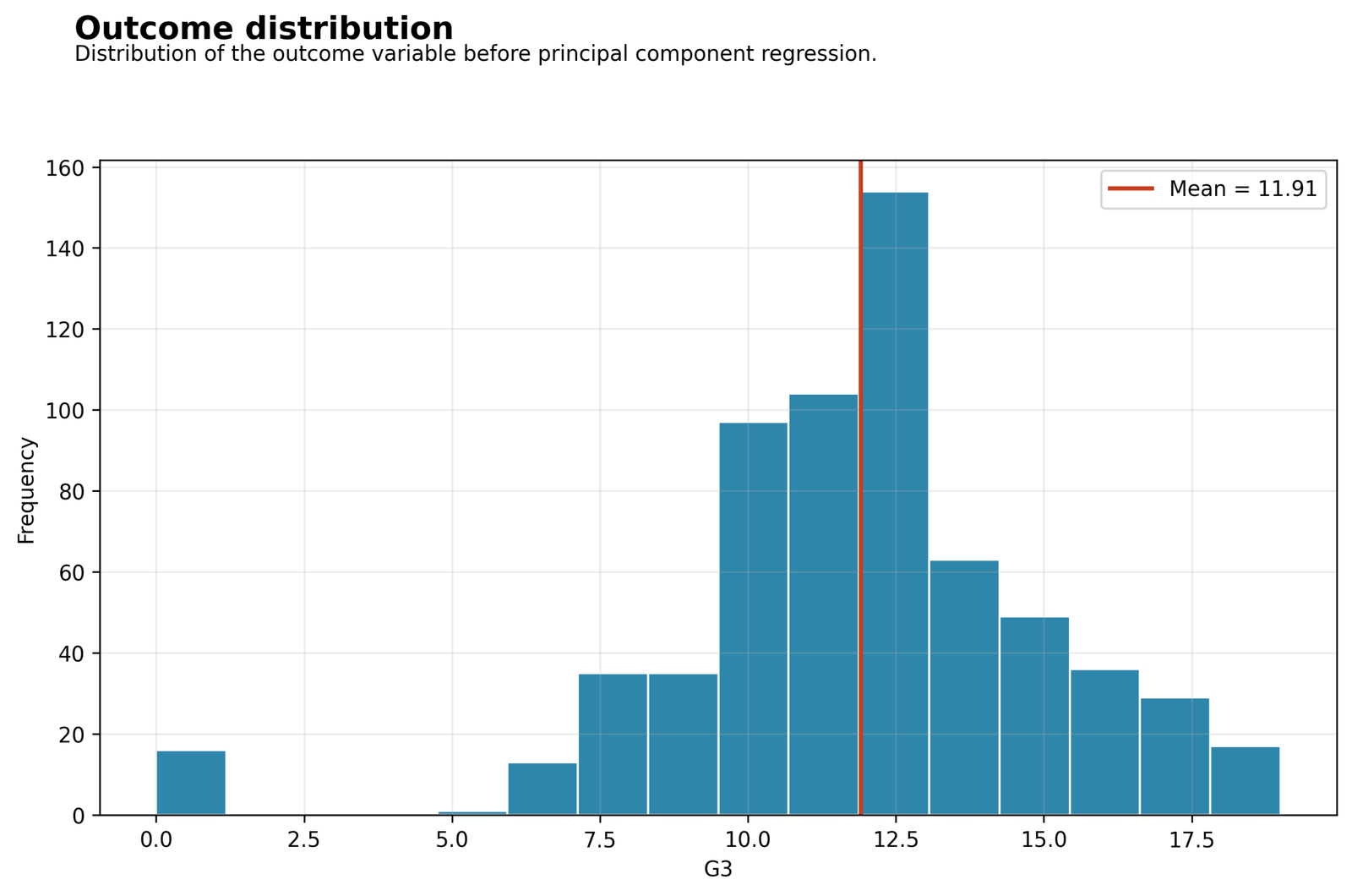
The histogram displays the 649 observed G3 values. Most grades are concentrated from approximately 9 to 15, while a small cluster occurs at zero.
The mean is approximately 11.91. G3 ranges from 0 to 19, and the fitted model uses all 649 observations.
The isolated zero-grade group creates a longer lower tail. Principal Component Regression predicts a continuous conditional mean, so these observations can produce large negative residuals if their predictor profiles resemble higher-grade students.
Inspect residuals for the zero cases and verify that they are valid observations. Do not delete them solely because they are difficult to predict.
Python Chart 2: Principal Component Regression Scree Plot
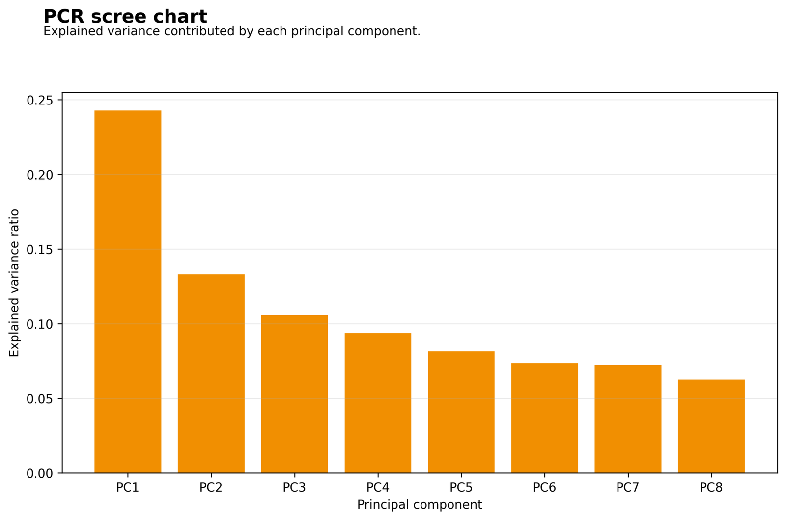
The bars show the marginal fraction of standardized predictor variance explained by each component. The declining pattern is expected because PCA orders components by variance.
PC1 explains 24.28%, PC2 13.32%, PC3 10.56%, PC4 9.36%, PC5 8.16%, PC6 7.37%, PC7 7.23% and PC8 6.27%.
No single component dominates the predictor space. The first two components together retain only 37.59%, so a two-component solution would discard most standardized predictor variation.
Use predictive validation rather than choosing the component count from the scree shape alone. The outcome may depend on later directions.
Python Chart 3: Principal Component Regression Cross-Validated RMSE
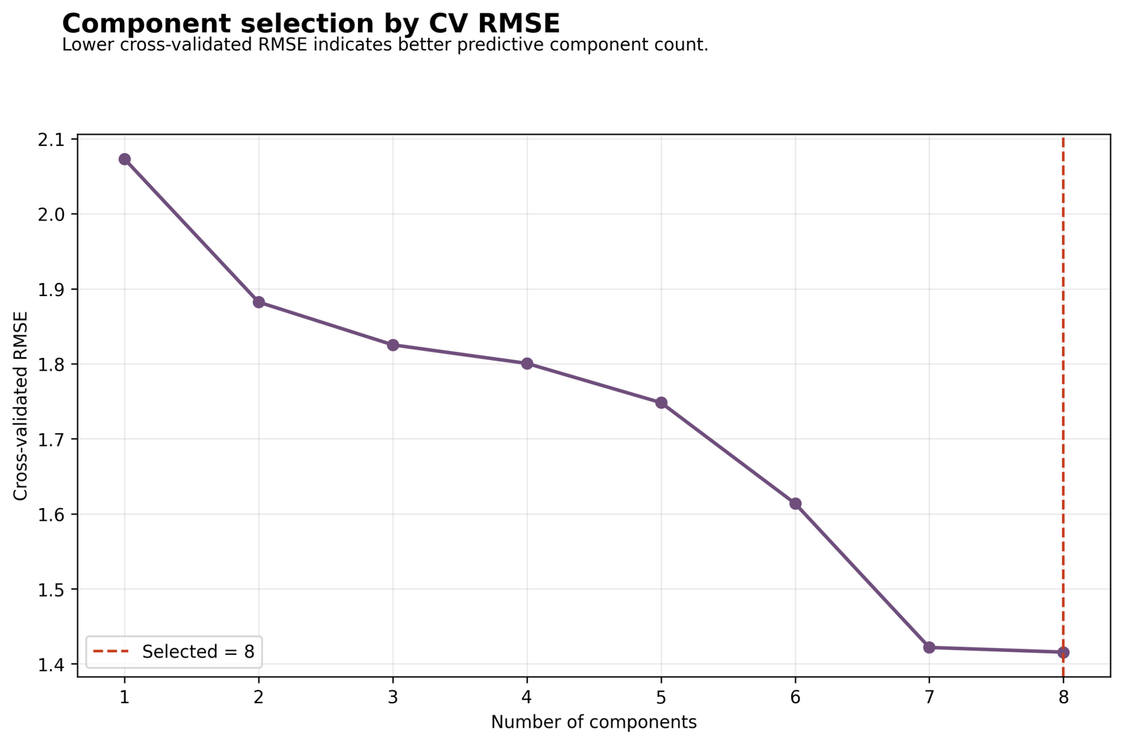
The curve compares prediction error for models using one through eight components. Error declines steadily, with a pronounced improvement from six to seven components.
RMSE declines from 2.0730 with one component to 1.6137 with six, 1.4219 with seven and 1.4157 with eight.
The eighth component provides only a modest improvement over the seventh, but it is selected under the stated minimum-RMSE rule. Cross-validated R² at eight components is 0.8077.
Repeat cross-validation with several fold allocations. Report whether seven and eight components have practically indistinguishable error.
Python Chart 4: Principal Component Regression Observed Versus Predicted Values
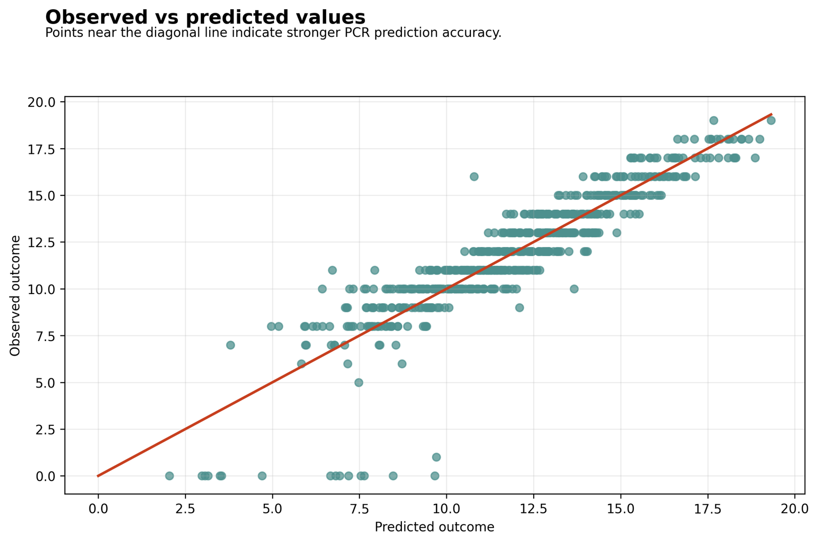
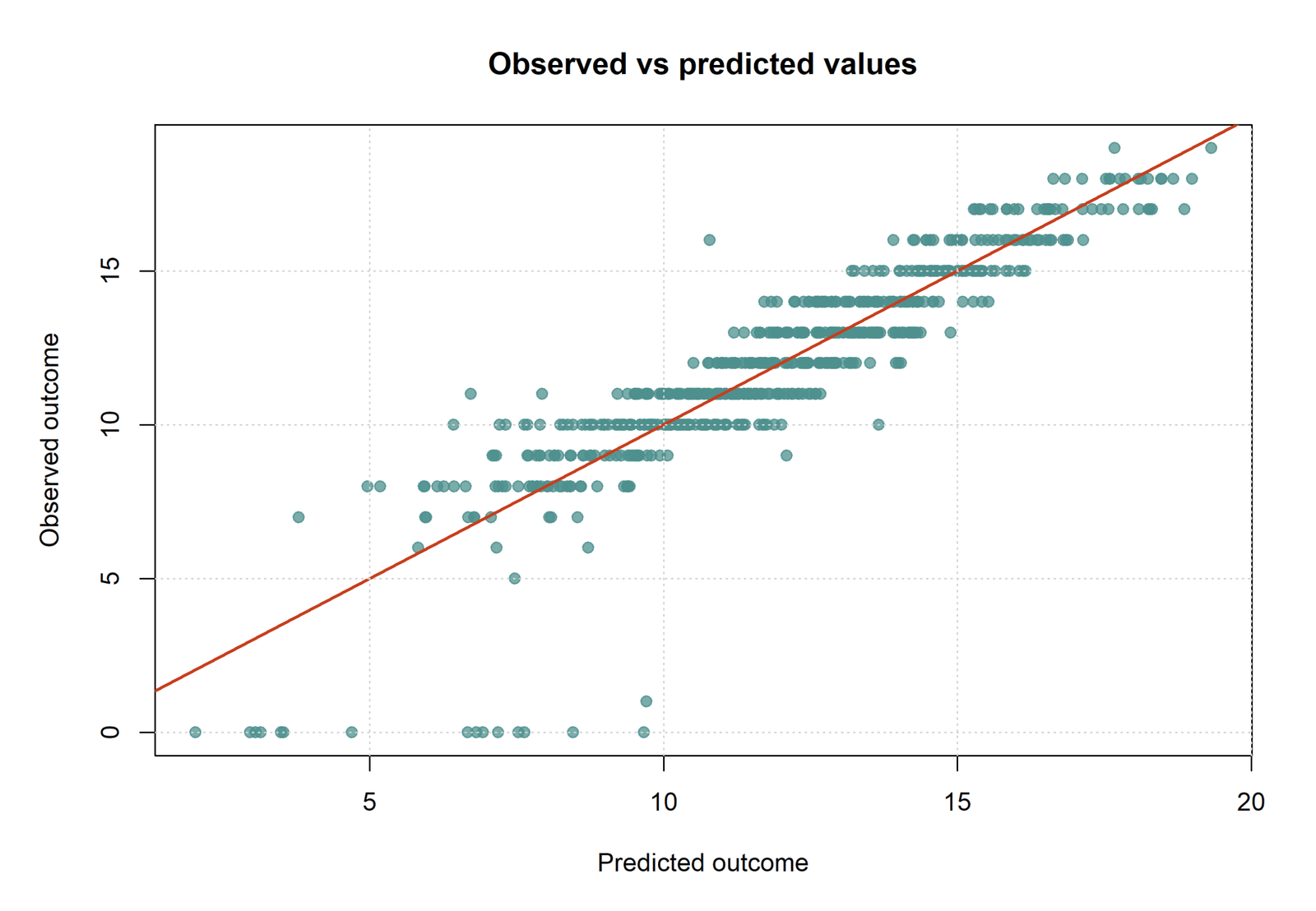
The horizontal grade bands reflect the integer-valued G3 outcome. Most points follow the diagonal, especially across the central grade range.
Training R² = 0.812203, adjusted R² = 0.809856, RMSE = 1.398943 and MAE = 0.905775.
The selected model captures most grade ordering but tends to pull extreme outcomes toward the center. Several observed zeros receive much higher predictions and create large negative residuals.
Validate on unseen data and compare error with ordinary least squares, partial least squares, Lasso Regression and a simpler seven-component model.
R Charts and Explanations
The R visuals use the same 649 rows and eight-component solution. The supplied R chart files are paired so each graph is followed by its corresponding explanation on desktop and mobile screens.
R Chart 1: Observed Versus Predicted
Most observations fall near the diagonal, consistent with R² = 0.8122. Prediction is strongest in the dense middle of the grade distribution. Extreme low outcomes show greater error because linear fitted values are pulled toward the sample center.
R Chart 2: Residuals Versus Fitted
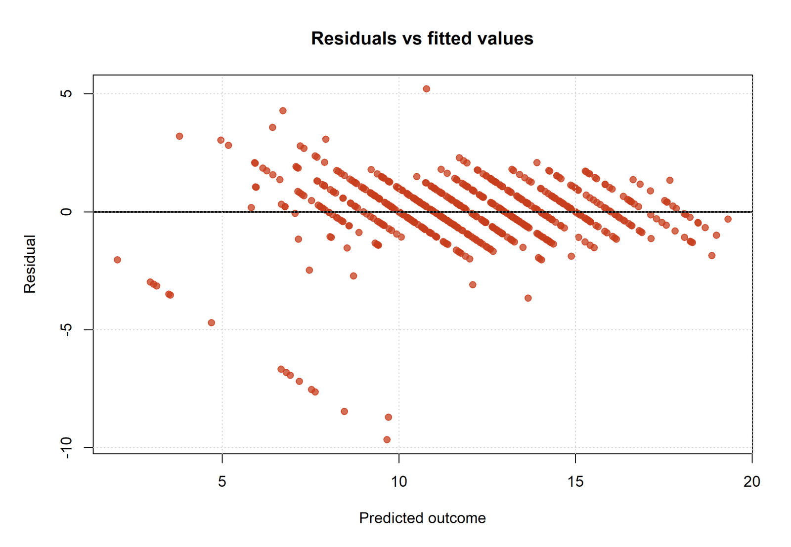
Residuals are broadly centered around zero, but diagonal bands appear because G3 takes integer values. Several negative residuals extend below −8, corresponding to observed grades that are much lower than predicted.
Cumulative Predictor Variance
- PC1: 24.28%
- PC1–PC2: 37.59%
- PC1–PC4: 57.52%
- PC1–PC6: 73.05%
- PC1–PC7: 80.28%
- PC1–PC8: 86.55%
R Chart 3: PC1 and PC2 Score Map
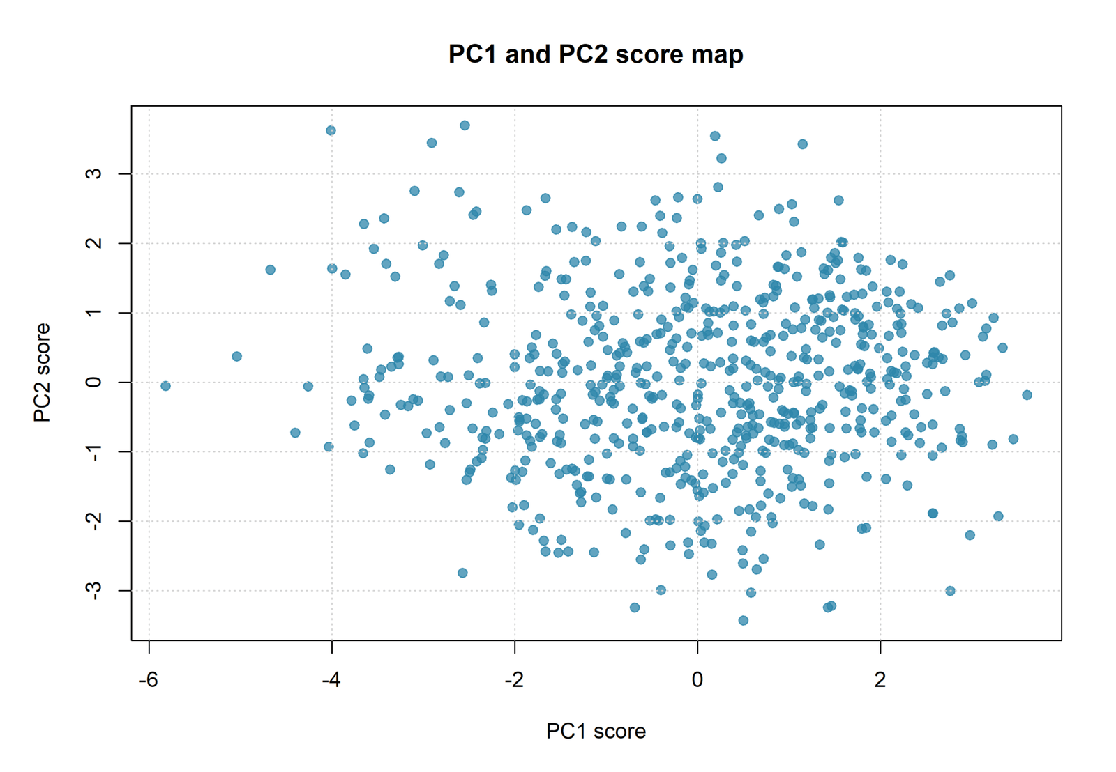
Higher G3 values tend to appear toward the positive PC1 direction, while lower grades are more common toward negative PC1. PC1 alone explains 24.28% of predictor variance and is strongly loaded by G1 and G2.
R Chart 4: Cumulative Variance Summary
The cumulative percentage rises to 57.52% after four components, 73.05% after six, 80.28% after seven and 86.55% after eight. The chart explains why a very small component set would omit substantial predictor information.
Principal Component Regression Coefficient Interpretation
Component-space slopes describe the relationship between G3 and each retained component score, conditional on the other retained components. Original-scale coefficients are reconstructed from the loading matrix, component coefficients and predictor scaling. The reconstructed values are easier to communicate, but they remain products of the entire Principal Component Regression transformation.
| Term | Original-scale coefficient | Standardized-predictor coefficient | Interpretation |
|---|---|---|---|
| G1 | 0.494354 | 1.356088 | Higher first-period grade is associated with higher predicted G3 in the reconstructed equation. |
| G2 | 0.484717 | 1.411202 | G2 has the largest standardized reconstructed coefficient and is a dominant positive predictor. |
| studytime | −0.069432 | −0.057550 | The conditional reconstructed coefficient is slightly negative after the full component structure is considered. |
| failures | −0.707365 | −0.419310 | Previous failures have the largest negative original-scale reconstructed coefficient. |
| absences | −0.005446 | −0.025253 | Each additional absence has a small negative reconstructed contribution. |
| age | 0.262102 | 0.319030 | Age has a positive derived coefficient in this selected component solution. |
| Medu | 0.015300 | 0.017345 | The reconstructed association is close to zero. |
| Fedu | −0.028179 | −0.030971 | The reconstructed association is small and negative. |
| school_MS | −0.573307 | −0.273128 | MS has a lower predicted value than GP within the reconstructed model. |
| sex_M | −0.275694 | −0.135589 | Male has a lower reconstructed predicted value than female. |
| address_U | −0.095369 | −0.043850 | Urban address has a small negative coefficient relative to rural. |
| famsize_LE3 | 0.035845 | 0.016360 | Family size of three or fewer has a near-zero positive coefficient. |
Predictions, Loadings and Component Meaning
Principal Component Loadings and Component Meaning
Loadings show how strongly each standardized predictor contributes to a component. The sign of every component is arbitrary: multiplying all loadings and scores for one component by −1 gives an equivalent PCA solution. Interpretation should therefore focus on relative signs and magnitudes within a component rather than treating the orientation as inherently positive or negative.
| Predictor | PC1 loading | Interpretive role on PC1 |
|---|---|---|
| G1 | 0.479278 | Largest positive contribution. |
| G2 | 0.471359 | Second-largest positive contribution. |
| Medu | 0.346955 | Positive education contribution. |
| Fedu | 0.317921 | Positive education contribution. |
| studytime | 0.212977 | Moderate positive contribution. |
| address_U | 0.207454 | Moderate positive contribution. |
| age | −0.187576 | Negative contribution. |
| school_MS | −0.294246 | Substantial negative contribution. |
| failures | −0.329453 | Largest negative contribution. |
PC1 can be described cautiously as a broad academic-achievement and education direction: higher G1, G2 and parental education align with positive scores, while failures and school_MS align negatively. This interpretation is supported by the score map, where higher G3 values tend to occur toward positive PC1.
Later components isolate different contrasts. PC4 is strongly related to famsize_LE3 at 0.6598. PC5 loads heavily on age at 0.5871 and famsize_LE3 at 0.5293. PC6 contrasts absences at 0.5661 with studytime at −0.5178 and address_U at −0.4402. PC7 loads strongly on sex_M at 0.4950 and negatively on famsize_LE3 at −0.4448. PC8 contrasts studytime at 0.5865 and sex_M at 0.4554 with address_U at −0.5265.
Worked Principal Component Regression Excel Calculation
The worked workbook contains Model Fit, Component Variance, CV Selection, Coefficients, Component Coefficients, Component Loadings, Worked Data Sample, Prediction Calculator and PCR Formula Guide sheets. The prediction calculator uses the reconstructed original-scale equation for an easy hand-check.
| Input | Example value | Coefficient | Contribution |
|---|---|---|---|
| Intercept | 1 | −3.020182 | −3.020182 |
| G1 | 12 | 0.494354 | 5.932253 |
| G2 | 11 | 0.484717 | 5.331887 |
| studytime | 2 | −0.069432 | −0.138864 |
| failures | 0 | −0.707365 | 0 |
| absences | 4 | −0.005446 | −0.021783 |
| age | 18 | 0.262102 | 4.717827 |
| Medu | 4 | 0.015300 | 0.061200 |
| Fedu | 4 | −0.028179 | −0.112715 |
| school_MS | 0 | −0.573307 | 0 |
| sex_M | 0 | −0.275694 | 0 |
| address_U | 1 | −0.095369 | −0.095369 |
| famsize_LE3 | 0 | 0.035845 | 0 |
| Predicted G3 | 12.6543 | ||
For a true component-score worksheet, standardize each predictor with =(raw value − training mean) / training SD, compute each score with SUMPRODUCT across standardized predictors and the relevant loading column, and then multiply the selected score columns by their component regression coefficients. The reconstructed calculator is easier to use, but the component-score method is better for auditing every stage of Principal Component Regression.
Principal Component Regression Assumptions and Diagnostics
The residual is observed G3 minus predicted G3. The fitted model has residual mean effectively equal to zero because an intercept is included. The residual histogram is concentrated around zero, while a small number of cases extend to approximately −10 and +5. These extremes deserve review because they can affect RMSE and the apparent quality of the selected component count.
What looks acceptable
- Most residuals fall within approximately −2 to +2.
- The main residual mass is centered near zero.
- The observed-versus-predicted relationship is strongly positive.
- No obvious broad curve dominates the residual-versus-fitted display.
What requires caution
- Several zero-grade observations have residuals below −6.
- Integer outcomes create diagonal residual bands.
- Fitted-sample R² may overstate generalization.
- Nonconstant tail behavior may affect conventional intervals.
Principal components eliminate exact sample correlation among the score columns, but they do not guarantee a correct outcome model. Analysts should still examine leverage, Cook’s distance, heteroscedasticity, nonlinear relationships and subgroup error. A robust or nonlinear model may improve prediction if the same observations remain poorly fitted under repeated validation.
Principal Component Regression in Python, R, SPSS and Excel
Python
Use pandas for data preparation, ColumnTransformer for numeric scaling and dummy coding, PCA for component scores and LinearRegression for the regression stage. GridSearchCV or a custom cross-validation loop can select the number of components.
- Keep preprocessing inside Pipeline.
- Use the same folds for every component count.
- Store loadings, means and standard deviations.
- Report validation and final-fit metrics separately.
R
Use model.matrix for indicator coding and either prcomp plus lm or the pls package. A manual prcomp workflow gives direct control over component loadings and coefficient reconstruction.
- Use scale = TRUE.
- Select ncomp with cross-validation.
- Inspect scores and loadings.
- Reconstruct coefficients carefully.
SPSS
SPSS can save principal component scores with FACTOR and then use REGRESSION with the selected score variables. This is a transparent teaching workflow even when automatic component-count cross-validation is performed in Python or R.
- Create indicator variables first.
- Extract principal components from the correlation matrix.
- Save eight component scores.
- Regress G3 on FAC1_1 through FAC8_1.
Excel
Excel can calculate standardized values, component scores, fitted values and residuals when the loadings and component coefficients are supplied. The attached worked workbook also provides reconstructed original-scale coefficients and a prediction calculator.
- Store means and SDs once.
- Use SUMPRODUCT for component scores.
- Use SUMPRODUCT for the final prediction.
- Protect formula cells before distribution.
Code: Expand Only the Software You Need
Python Principal Component Regression
import pandas as pd
from sklearn.compose import ColumnTransformer
from sklearn.preprocessing import StandardScaler, OneHotEncoder
from sklearn.decomposition import PCA
from sklearn.linear_model import LinearRegression
from sklearn.pipeline import Pipeline
from sklearn.model_selection import GridSearchCV, KFold
from sklearn.metrics import mean_squared_error, mean_absolute_error, r2_score

# Load the dataset.
df = pd.read_csv("dataset.csv", sep=None, engine="python")
y = df["G3"]
numeric = ["G1", "G2", "studytime", "failures", "absences", "age", "Medu", "Fedu"]
categorical = ["school", "sex", "address", "famsize"]
X = df[numeric + categorical]

prep = ColumnTransformer([
    ("num", StandardScaler(), numeric),
    ("cat", OneHotEncoder(drop="first", handle_unknown="ignore"), categorical),
])

pipe = Pipeline([
    ("prep", prep),
    ("pca", PCA()),
    ("reg", LinearRegression()),
])

cv = KFold(n_splits=5, shuffle=True, random_state=42)
search = GridSearchCV(
    pipe,
    {"pca__n_components": list(range(1, 9))},
    scoring="neg_root_mean_squared_error",
    cv=cv,
)
search.fit(X, y)

best_model = search.best_estimator_
pred = best_model.predict(X)
print("Selected components:", search.best_params_["pca__n_components"])
print("RMSE:", mean_squared_error(y, pred) ** 0.5)
print("MAE:", mean_absolute_error(y, pred))
print("R-squared:", r2_score(y, pred))
R Principal Component Regression
dat <- read.csv("dataset.csv", check.names = FALSE)
y <- dat$G3
x <- model.matrix(
  ~ G1 + G2 + studytime + failures + absences + age + Medu + Fedu +
    school + sex + address + famsize,
  data = dat
)[, -1]

pca <- prcomp(x, center = TRUE, scale. = TRUE)
scores <- pca$x
selected <- 8
pcr_data <- data.frame(G3 = y, scores[, 1:selected, drop = FALSE])
fit <- lm(G3 ~ ., data = pcr_data)
pred <- predict(fit)

rmse <- sqrt(mean((y - pred)^2))
mae <- mean(abs(y - pred))
r2 <- summary(fit)$r.squared
adj_r2 <- summary(fit)$adj.r.squared

print(summary(fit))
cat("Selected components:", selected, "\n")
cat("RMSE:", rmse, " MAE:", mae, " R2:", r2, " Adj R2:", adj_r2, "\n")
SPSS Principal Component Regression
* Create the four indicator variables before FACTOR.
COMPUTE school_MS = (school = 'MS').
COMPUTE sex_M = (sex = 'M').
COMPUTE address_U = (address = 'U').
COMPUTE famsize_LE3 = (famsize = 'LE3').
EXECUTE.

FACTOR
 /VARIABLES G1 G2 studytime failures absences age Medu Fedu
            school_MS sex_M address_U famsize_LE3
 /MISSING LISTWISE
 /ANALYSIS G1 G2 studytime failures absences age Medu Fedu
           school_MS sex_M address_U famsize_LE3
 /PRINT INITIAL EXTRACTION
 /CRITERIA FACTORS(8) ITERATE(25)
 /EXTRACTION PC
 /ROTATION NOROTATE
 /SAVE REG(ALL)
 /METHOD=CORRELATION.

REGRESSION
 /DEPENDENT G3
 /METHOD=ENTER FAC1_1 FAC2_1 FAC3_1 FAC4_1 FAC5_1 FAC6_1 FAC7_1 FAC8_1
 /STATISTICS COEFF OUTS R ANOVA CI(95)
 /SAVE PRED(PCR_PRED) RESID(PCR_RESID).
Excel Principal Component Regression Logic
Standardized predictor:
=(B2-$B$653)/$B$654

PC1 score when standardized predictors are in B2:M2 and PC1 loadings are in B660:M660:
=SUMPRODUCT(B2:M2,$B$660:$M$660)

Predicted G3 from PC1:PC8 scores and component coefficients:
=$B$670+SUMPRODUCT(N2:U2,$N$671:$U$671)

Residual:
=Observed_G3-Predicted_G3

RMSE:
=SQRT(SUMSQ(Residual_Range)/COUNT(Residual_Range))
Advanced Principal Component Regression Topics
Why nested cross-validation matters
When the number of components is selected by cross-validation, the reported prediction error should come from an outer validation process that was not used to choose that component count. In a nested design, inner folds choose the number of components and outer folds estimate performance. This prevents the same validation observations from influencing both model tuning and model evaluation. The worked example reports the available five-fold component-selection error and separately labels the full-sample fit statistics, but a final production model should preferably add an outer test or nested cross-validation layer.
Principal Component Regression when predictors exceed observations
Principal Component Regression can fit a lower-dimensional score model even when the original predictor count is greater than the number of observations. The maximum useful number of nonzero components is limited by matrix rank, and component selection becomes especially important. All centering, scaling, dummy coding and missing-value handling must be learned within each training fold. Otherwise information from held-out observations leaks into the components and makes validation error look too optimistic.
Why scaling changes the model
PCA follows variance. Without standardization, a predictor measured on a large numerical scale can dominate component extraction even when it is not substantively more important. Standardizing every numeric and indicator column gives each column unit sample variance, but this is not automatically ideal for every research problem. Binary indicators can receive large standardized values when one category is rare. The scaling rule should therefore be stated, justified and reproduced in Python, R, SPSS and Excel.
How coefficient reconstruction works
The score regression estimates a coefficient for every retained component. Multiplying the loading matrix by the component coefficient vector maps the model back to standardized predictor space. Dividing by the original predictor standard deviations and correcting the intercept maps the result to the original scale. These reconstructed coefficients reproduce predictions when the same means, standard deviations, coding and retained components are used. They are useful summaries, but they are not identical to direct OLS slopes and should not be presented as independent causal effects.
Bootstrap stability of loadings and predictions
Loadings can change across samples, especially when eigenvalues are close. A bootstrap analysis can repeatedly resample rows, rerun the complete Principal Component Regression pipeline and summarize prediction error, retained component counts and reconstructed coefficients. Component signs must be aligned before averaging because each component can reverse sign without changing the underlying solution. Stability analysis is particularly useful when readers might otherwise overinterpret small loadings or small reconstructed coefficients.
Principal Component Regression for non-Gaussian outcomes
The standard model in this guide uses linear regression for continuous G3. For binary, count, ordinal or survival outcomes, researchers sometimes use selected principal component scores inside logistic, Poisson, ordinal or survival models. That extension changes the loss function, metrics, diagnostics and interpretation. It should be described as a generalized model using principal components rather than treated as identical to the continuous-outcome Principal Component Regression procedure shown here.
Principal Component Regression Compared with Other Methods
| Method | How predictors are handled | Main strength | Main limitation |
|---|---|---|---|
| Ordinary least squares | Uses original predictors directly. | Direct coefficient interpretation. | Can be unstable under strong multicollinearity. |
| Principal Component Regression | Creates PCA components without using the outcome, then regresses on selected scores. | Orthogonal predictors and dimension reduction. | High-variance components are not necessarily the most predictive. |
| Partial least squares regression | Creates latent scores using both predictor and outcome structure. | Often efficient for prediction when outcome-related directions have modest X variance. | Latent components can be harder to interpret and tune. |
| Lasso Regression | Shrinks original coefficients and can set some exactly to zero. | Sparse variable selection. | Selection can be unstable among highly correlated predictors. |
| Ridge regression | Shrinks all original slopes toward zero. | Stable prediction with correlated variables. | Does not ordinarily produce exact zeros. |
| Elastic Net Regression | Combines L1 and L2 penalties. | Balances grouped retention and sparsity. | Requires tuning two penalty dimensions. |
Principal Component Regression differs from principal component analysis because PCA is only the predictor-transformation stage. PCR adds a supervised regression step. It differs from multiple linear regression because the actual fitted predictors are component scores rather than the original variables. It differs from partial least squares because PCA does not look at G3 while creating components.
Common Principal Component Regression Mistakes
Model-building mistakes
- Running PCA before the train/test split.
- Standardizing the full dataset before cross-validation.
- Choosing components only from an explained-variance threshold.
- Using different dummy references across software.
- Comparing candidate models with different folds or preprocessing.
- Allowing the outcome G3 to enter the PCA predictor matrix.
Interpretation mistakes
- Calling 86.55% retained predictor variance an R² value.
- Treating reconstructed coefficients as causal effects.
- Reading a component sign as inherently positive or negative.
- Reporting training RMSE as future prediction performance.
- Ignoring residual outliers because component scores are orthogonal.
- Assuming the first components must be the best outcome predictors.
A defensible Principal Component Regression analysis keeps the entire workflow together: coding, centering, scaling, PCA, component selection and regression are all parts of one model pipeline. Any step learned from held-out data can leak information. Any comparison that changes more than one feature at a time can misattribute performance differences.
APA-Style Reporting
A complete Principal Component Regression report should identify the outcome, original predictors, dummy references, standardization rule, PCA implementation, cross-validation folds, candidate component range, selection criterion, final component count and retained predictor variance. It should then report outcome metrics separately. Do not use the phrase “explained variance” without stating whether it refers to X-space component variance or G3 outcome variance.
The fitted R², adjusted R², RMSE and MAE above describe the final model on the 649-row sample. The cross-validated RMSE describes component-selection performance under the specified folds. A separate untouched test set or nested cross-validation would provide the strongest estimate of future generalization.
Publication Checklist
Model construction
- Define G3 as the outcome.
- List all original predictors and dummy references.
- Standardize predictors using training information.
- Run PCA on predictors only.
- Select the component count with cross-validation.
- Save the seed and fold assignments.
Reporting and validation
- Report component-specific and cumulative variance.
- Report CV RMSE for candidate component counts.
- Report final R², adjusted R², RMSE and MAE.
- Explain reconstructed coefficients cautiously.
- Show observed-versus-predicted and residual plots.
- Compare with at least one alternative model.
Downloads and Chart Resources
Principal Component Regression R ReportR validation results, component variance, loadings, fitted metrics and reconstructed coefficients
Frequently Asked Questions
What is Principal Component Regression?
Principal Component Regression runs PCA on centered and usually standardized predictors, retains a validated number of component scores and fits linear regression using those scores.
Why use Principal Component Regression instead of ordinary regression?
It can reduce dimensions and stabilize prediction when original predictors are strongly correlated. The trade-off is that original-variable interpretation becomes indirect.
How many components should be used?
Select the count with cross-validation when prediction is the objective. In this example, eight components produce the lowest available five-fold cross-validated RMSE among one through eight components.
Is 86.55% explained variance the model R-squared?
No. The 86.55% value is cumulative variance retained from the standardized predictor matrix. The fitted G3 outcome R² is 0.8122, or 81.22%.
Does Principal Component Regression solve multicollinearity?
It replaces correlated original columns with orthogonal component scores, so retained regression predictors are uncorrelated in the fitted sample. It does not solve omitted variables, nonlinear form, outliers, heteroscedasticity or data leakage.
What is the difference between Principal Component Regression and Partial Least Squares Regression?
PCR constructs components to explain predictor variance without looking at G3. PLS constructs latent directions with reference to both predictors and outcome. PLS may therefore retain an outcome-relevant direction even when that direction explains comparatively little predictor variance.
Can Principal Component Regression be used in Python?
Yes. A safe scikit-learn workflow combines preprocessing, PCA and LinearRegression inside one Pipeline and tunes pca__n_components with GridSearchCV or nested cross-validation.
Can Principal Component Regression be used in R?
Yes. Use model.matrix with prcomp and lm for a transparent workflow, or use a PCR-capable package with cross-validation. Report scaling and component-selection settings.
Can Principal Component Regression be used in SPSS?
Yes. Create indicators, extract and save principal component scores with FACTOR, then regress G3 on the retained FAC variables. Component-count validation is usually easier to automate in Python or R.
Can Principal Component Regression be calculated in Excel?
Yes, once means, standard deviations, loadings and component coefficients are available. SUMPRODUCT can calculate scores and predictions. The supplied workbook includes model-fit, variance, CV, coefficient, loading and prediction sheets.
Can categorical variables be included?
Yes, after explicit indicator coding. The reference category and scaling of each indicator must remain identical across training, validation, software and future prediction data.
Are reconstructed coefficients the same as OLS coefficients?
No. Reconstructed PCR coefficients combine retained component loadings with component regression slopes. They reproduce the selected PCR prediction rule but need not match direct OLS slopes.
What do the largest reconstructed coefficients show?
G1 and G2 have the largest positive original-scale coefficients, while failures and school_MS have the largest negative coefficients in the eight-component solution.
What performance should be reported?
Report cross-validated component-selection error and separately report final R², adjusted R², RMSE and MAE. State whether each metric is training, validation, test or nested-CV performance.
Is Principal Component Regression a machine-learning method?
It can be treated as a supervised machine-learning pipeline because component count is tuned to predict an outcome. It is also a classical multivariate regression technique.
Principal Component Regression Conclusion
Principal Component Regression provides a practical bridge between principal component analysis and predictive regression. It is most valuable when correlated predictors make direct slopes unstable, the analyst can justify standardization, and component count is selected within a valid resampling procedure.
In the 649-observation worked model, eight components retain 86.55% of standardized predictor variance. The available five-fold cross-validation results reach their lowest RMSE at eight components, with Python CV RMSE = 1.4157. The fitted final model has R² = 0.8122, adjusted R² = 0.8099, RMSE = 1.3989 and MAE = 0.9058. G1 and G2 dominate the positive reconstructed prediction, while failures and school_MS provide the largest negative reconstructed terms.
The strongest conclusion is not that PCA automatically improves every regression. The evidence shows that a validated eight-component representation preserves most predictor information and produces strong fitted prediction for G3, while residual outliers and the difference between training and validation metrics still require careful reporting. A fair comparison with OLS, PLS, ridge, Lasso and Elastic Net should use the same preprocessing, folds and evaluation metric.

