
Polynomial Regression: Formula, Interpretation, Python, R, SPSS and Excel Guide
Polynomial Regression extends a linear model by adding squared, cubic, or higher-degree predictor terms. This worked analysis compares linear, quadratic, and cubic models for predicting G3 from centered G2 while adjusting for academic and background covariates.
G3 outcome
G2 polynomial predictor
Best adjusted R² 0.851767
Polynomial Regression Model Overview
Polynomial Regression is a regression method for relationships that cannot be represented adequately by one straight line. It adds powers of a predictor—such as X² and X³—to an ordinary regression equation so the fitted response can bend, flatten, accelerate, or change direction. The method is used for a continuous dependent variable when theory, plots, or diagnostics suggest that the effect of a predictor changes across its range.
Definition of Polynomial Regression
Polynomial Regression is a special case of Multiple Linear Regression in which transformed versions of the same predictor enter the model as separate terms. A quadratic model contains X and X². A cubic model contains X, X², and X³. Higher-degree models can be written in the same way, although increasing degree also increases the risk of overfitting, unstable coefficients, and implausible behavior near or beyond the data boundaries.
The word polynomial refers to a sum of powers. The word regression indicates that the model estimates the conditional mean of a dependent variable from one or more predictors. The model can also include ordinary covariates, categorical indicators, interactions, and other transformations alongside the polynomial terms.
Is Polynomial Regression Linear or Nonlinear?
Polynomial Regression produces a nonlinear curve in X, but it is still a linear model in its unknown coefficients. The equation is linear in β₀, β₁, β₂, and β₃ even though it includes nonlinear functions of X. That means Polynomial Regression can be fitted with ordinary least squares and interpreted with familiar regression statistics when the usual error assumptions are appropriate.
This distinction separates Polynomial Regression from genuinely Nonlinear Regression models in which the parameters themselves enter the equation nonlinearly. A model such as Y = β₀ + β₁X + β₂X² remains linear in β. A model such as Y = β₀ exp(β₁X) is nonlinear in its parameters.
What Question Does Polynomial Regression Answer?
Polynomial Regression answers whether the expected outcome changes along a curved path as a predictor varies. It can show whether the outcome rises quickly and then levels off, falls and then rises, reaches a peak, approaches a plateau, or follows another smooth shape that a single straight-line coefficient would conceal.
The analysis also asks whether additional powers materially improve fit. A quadratic term tests whether one bend improves the model beyond a straight line. A cubic term allows more flexibility and can represent an S-shaped tendency or a change in curvature. Degree selection should consider fit statistics, validation error, theory, and parsimony together.
When Polynomial Regression Is Used
Polynomial Regression is used when a scatterplot or substantive theory suggests curvature, when residuals from a linear model contain a systematic curve, or when the marginal effect of a predictor is expected to change across its range. Applications include growth, dose-response patterns, learning curves, economic cost relationships, engineering calibration, environmental exposure, biological development, and machine-learning prediction.
The method is appropriate only when the observed range contains enough information to estimate the curve reliably. Polynomial Regression is not a general license to fit very high degrees. A high-degree curve may pass closely through training observations while behaving erratically between them or outside the sample range.
Why Polynomial Regression Is Used Instead of a Straight Line
A straight-line model assumes that a one-unit predictor change has the same expected outcome effect everywhere. That is often unrealistic. The difference between G2 scores of 5 and 6 may not carry the same final-grade implication as the difference between 17 and 18. Polynomial Regression allows the slope to change with G2.
The present model finds a positive first-order G2 term and a negative squared term. Together they describe a relationship that rises strongly but flattens slightly at higher values. The curve remains increasing throughout the observed range, so the model does not imply that higher G2 eventually reduces G3 within the available data.
Core Polynomial Regression Formula
This is a second-degree or quadratic Polynomial Regression model. A third-degree model adds X³:
With covariates Z₁ through Zₘ, the equation becomes:
Why the Predictor Is Centered
Raw polynomial powers are often highly correlated. Centering replaces X with X − X̄ before creating squared and cubic terms. In this analysis, G2 is centered at 11.5701079. The centered variable equals zero at the sample mean, making the intercept more interpretable and reducing unnecessary numerical dependence among powers.
Centering does not change the fitted curve or predictions when all required terms are included. It changes the numerical coefficients and their interpretation. The coefficient of the centered linear term describes the slope at the centering point, not one universal slope across the entire curve.
How Polynomial Coefficients Are Interpreted
Polynomial coefficients are not interpreted as isolated constant effects. In a cubic model, the instantaneous slope at a centered value z is:
The slope therefore depends on z. A positive β₁ does not mean the outcome rises at exactly β₁ units everywhere. The sign and magnitude of β₂ and β₃ alter the slope as the predictor changes. Predicted-value curves, marginal effects, and turning points are usually more informative than separate coefficient sentences.
How to Choose the Degree in Polynomial Regression
Degree selection should begin with theory and a limited candidate set. Analysts commonly compare linear, quadratic, and cubic forms using adjusted R², AIC, BIC, RMSE, MAE, nested-term tests, and cross-validation. The selected degree should improve fit enough to justify its additional flexibility.
In the present workbook, the cubic model has the highest adjusted R² and lowest RMSE. The quadratic model has the lowest AIC and MAE, and the cubic term is not statistically significant. The most accurate conclusion is therefore that the data support curvature, while the practical need for a third-degree term is weak.
Polynomial Regression Versus Multiple Linear Regression
Polynomial Regression is not an alternative to multiple linear regression in the way logistic or Poisson models are. It is a multiple linear regression containing transformed predictor columns. Ordinary least squares estimates the coefficients, and familiar concepts such as residuals, confidence intervals, R², F tests, and heteroskedasticity remain relevant.
Polynomial Regression Versus Nonlinear Regression
Nonlinear Regression is used when parameters enter the mean function nonlinearly or when a mechanistic function such as exponential growth is specified directly. Polynomial Regression is more flexible locally and easier to fit, but it may extrapolate poorly and lacks the direct scientific meaning of a well-chosen mechanistic curve.
Polynomial Regression in Machine Learning
In machine learning, Polynomial Regression is usually implemented by generating polynomial features and fitting a linear estimator. Python workflows often use PolynomialFeatures with LinearRegression, Ridge, Lasso, or Elastic Net. Cross-validation is essential because feature count grows rapidly as degree and predictor count increase.
A Polynomial Regression calculator can evaluate a fitted equation for new values, but it cannot determine whether the selected degree is valid. Degree choice, preprocessing, validation, and extrapolation limits must come from the complete analysis.
Supported Variable Types
The dependent variable is usually continuous. The polynomial predictor should be numeric. Additional predictors may be continuous, binary, ordinal, or categorical after appropriate coding. Interactions between polynomial terms and groups can test whether curves differ across categories.
Core Assumptions
- The conditional mean is represented adequately by the selected polynomial and covariates.
- Observations are independent unless a clustered extension is used.
- Residual variance is sufficiently stable or corrected with robust methods.
- Errors are approximately normal when classical small-sample inference is used.
- Influential observations do not determine the curve disproportionately.
- Polynomial powers are created consistently after centering or scaling.
- Predictions are not extrapolated far beyond the observed predictor range.
- The degree is chosen without using the final test sample repeatedly.
Advantages
- Captures smooth curvature while retaining linear-model estimation.
- Works with ordinary covariates and categorical predictors.
- Provides familiar fit statistics, residuals, and confidence intervals.
- Can be implemented in Python, R, SPSS, Excel, MATLAB, and other software.
- Offers an accessible bridge between straight-line regression and more flexible methods.
Limitations
- High degrees can overfit and oscillate.
- Raw powers can be highly collinear.
- Individual coefficients are difficult to interpret separately.
- Extrapolation can become unrealistic very quickly.
- Outliers near the predictor boundaries can alter the curve strongly.
- A polynomial may approximate a pattern without explaining the underlying mechanism.
Current Worked Scenario
The analysis uses 649 observations. G3 is the continuous outcome and G2 is the polynomial predictor. G2 is centered at 11.5701079. Covariates are G1, studytime, failures, absences, age, Medu, Fedu, traveltime, and health.
Three candidate models are fitted: a linear first-degree model, a quadratic second-degree model, and a cubic third-degree model. The workbook selects the cubic model by adjusted R². Its R² is 0.854512, adjusted R² is 0.851767, RMSE is 1.231316, and MAE is 0.763130.
The centered G2 term is positive, B = 0.866080, and the squared term is negative, B = −0.015395. The cubic term is small and uncertain, B = −0.000710, p = .22117. This pattern supports a strong increasing association with mild flattening rather than a complex third-degree shape.
Quick Answer
Model-selection result
- Highest adjusted R²: Cubic
- Lowest RMSE: Cubic
- Lowest AIC: Quadratic
- Lowest MAE: Quadratic
Curvature result
- Centered G2: B = 0.866080, p < .001
- G2 squared: B = −0.015395, p = .00125
- G2 cubed: B = −0.000710, p = .22117
Table of Contents
- Why this analysis needs Polynomial Regression
- How Polynomial Regression works
- Variables used and centering
- Linear, quadratic and cubic results
- Five Python chart stories
- Five R charts and explanations
- Coefficient interpretation
- Predictions, slopes and curve shape
- Assumptions and diagnostics
- Python, R, SPSS and Excel workflows
- Code
- Advanced Polynomial Regression topics
- APA-style reporting
- Publication checklist
- Downloads and chart resources
- Related Salar Cafe guides
- Frequently asked questions
Why This Analysis Needs Polynomial Regression
A straight-line model would force the expected G3 increase per G2 point to remain identical from the bottom to the top of the scale. The fitted curve indicates that G3 continues to rise, but its slope becomes slightly smaller at higher G2 values.
Polynomial Regression represents that pattern with centered G2, centered G2 squared, and centered G2 cubed. It remains an Ordinary Least Squares Regression model, but its transformed terms allow the mean response to bend.
The model is also preferable to choosing arbitrary G2 categories. Categorization would discard information, create artificial cut-points, and make results depend on those cut-points. Polynomial Regression retains the original numeric scale and estimates one smooth response function.
How Polynomial Regression Works
Subtract the G2 mean of 11.5701 to improve interpretation and numerical stability.
Calculate centered G2 squared and cubed for the candidate models.
Evaluate fit, error, parsimony, term evidence, and validation before selecting a curve.
The coefficient β₁ is the instantaneous slope at z = 0, which corresponds to mean G2. The squared and cubic coefficients change that slope as G2 moves away from the centering point.
All lower-order terms must remain in the model when a higher-order term is included. A cubic specification should contain z, z², and z³ even when one lower-order p-value is not below .05. This hierarchy preserves the meaning of the polynomial function.
Variables Used and Centering
| Variable | Role | Definition | Model use |
|---|---|---|---|
| G3 | Outcome | Final grade | Continuous dependent variable |
| G2 | Polynomial predictor | Second-period grade | Centered before powers are created |
| poly_x_centered | Polynomial term | G2 − 11.5701079 | First-order slope at the centering point |
| poly_x_centered_sq | Polynomial term | Centered G2 squared | Quadratic curvature |
| poly_x_centered_cu | Polynomial term | Centered G2 cubed | Third-degree flexibility |
| G1 | Covariate | First-period grade | Earlier academic performance |
| studytime | Covariate | Weekly study-time category | Study behavior |
| failures | Covariate | Previous failures | Academic difficulty |
| absences | Covariate | Absence count | Attendance |
| age | Covariate | Age in years | Demographic control |
| Medu, Fedu | Covariates | Mother’s and father’s education | Family education background |
| traveltime | Covariate | Home-to-school travel category | Logistical control |
| health | Covariate | Self-reported health | Health control |
Linear, Quadratic and Cubic Results
| Model | R² | Adjusted R² | AIC | BIC | RMSE | MAE | Interpretation |
|---|---|---|---|---|---|---|---|
| Linear | 0.851634 | 0.849308 | 2146.5889 | 2195.8187 | 1.243436 | 0.777900 | Strong baseline fit with a constant G2 slope |
| Quadratic | 0.854169 | 0.851651 | 2137.4030 | 2191.1082 | 1.232767 | 0.759566 | Meaningful curvature improvement and lowest AIC/MAE |
| Cubic | 0.854512 | 0.851767 | 2137.8744 | 2196.0550 | 1.231316 | 0.763130 | Highest adjusted R² and lowest RMSE, but minimal gain beyond quadratic |
Compared with linear
Improves parsimony-adjusted fit
Compared with quadratic
Worse than quadratic
Evidence of curvature
Limited evidence for degree three
Adjusted R² should be understood with the dedicated Adjusted R-Squared guide. Unlike raw R², it penalizes additional terms, but it can still favor a tiny improvement that has little practical value. AIC, BIC, validation error, and substantive interpretability remain necessary.
Worked Analysis Resource
The workbook supplied with this article contains the complete model-fit table, coefficient estimates, prediction sample, and polynomial calculator.
Five Python Chart Stories
The supplied Polynomial Regression figures are explained through the visible pattern, exact or appropriately rounded values, substantive interpretation, and their importance for model choice.
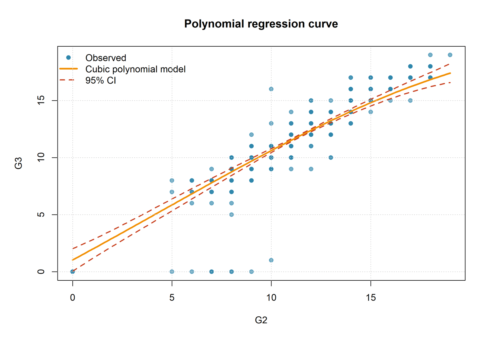
Chart 1: Polynomial Regression Curve with 95% Confidence Band
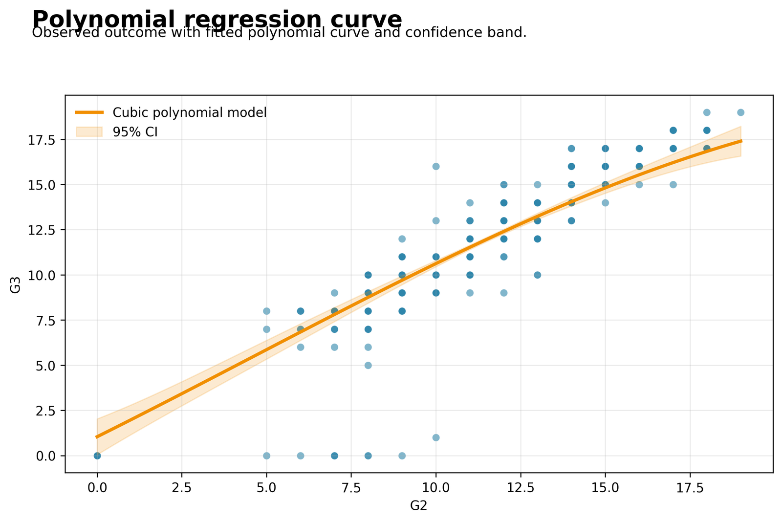
The fitted curve rises across the complete observed G2 range. It is close to linear through the central data cloud but gradually flattens at higher G2 values. The confidence band is narrowest in the densely observed middle and wider near the endpoints.
G2 is centered at 11.5701. With the other predictors held at their sample means, the cubic model predicts G3 of approximately 1.05 at G2 = 0, 10.64 at G2 = 10, 12.03 at the centered mean, 14.79 at G2 = 15, and 17.32 at G2 = 19.
The association is strongly positive, but the gain in predicted G3 becomes slightly smaller toward the upper end of G2. The negative squared coefficient produces most of that flattening. The cubic coefficient is small and uncertain, so the visible curve is not evidence of a complicated multi-turn relationship.
The curve communicates the combined polynomial effect better than any single coefficient. It also shows why predictions inside the observed range are more defensible than extrapolations beyond it.
Chart 2: Linear, Quadratic and Cubic Model Fit Comparison
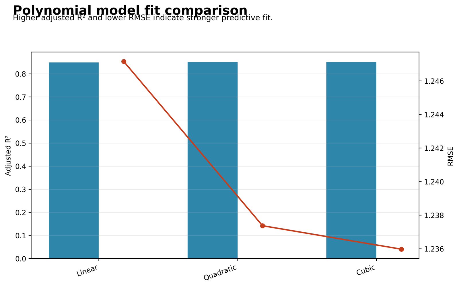
All three models fit strongly. The largest improvement occurs when the squared term is added to the linear model. The cubic model lowers RMSE only slightly beyond the quadratic model, while adjusted R-squared changes by a very small amount.
Linear: adjusted R² = 0.849308, RMSE = 1.243436, AIC = 2146.5889. Quadratic: adjusted R² = 0.851651, RMSE = 1.232767, AIC = 2137.4030. Cubic: adjusted R² = 0.851767, RMSE = 1.231316, AIC = 2137.8744.
The workbook’s adjusted-R-squared rule selects the cubic model, but the quadratic model has the lowest AIC and MAE. The cubic model improves adjusted R² by only 0.000116 beyond quadratic, and its cubic term has p = .221. The data therefore support curvature, while evidence for a necessary third-degree term is limited.
Polynomial degree should not be selected from training R² alone. This comparison shows the trade-off among fit, parsimony, error, and interpretability.
Chart 3: Observed Versus Predicted G3
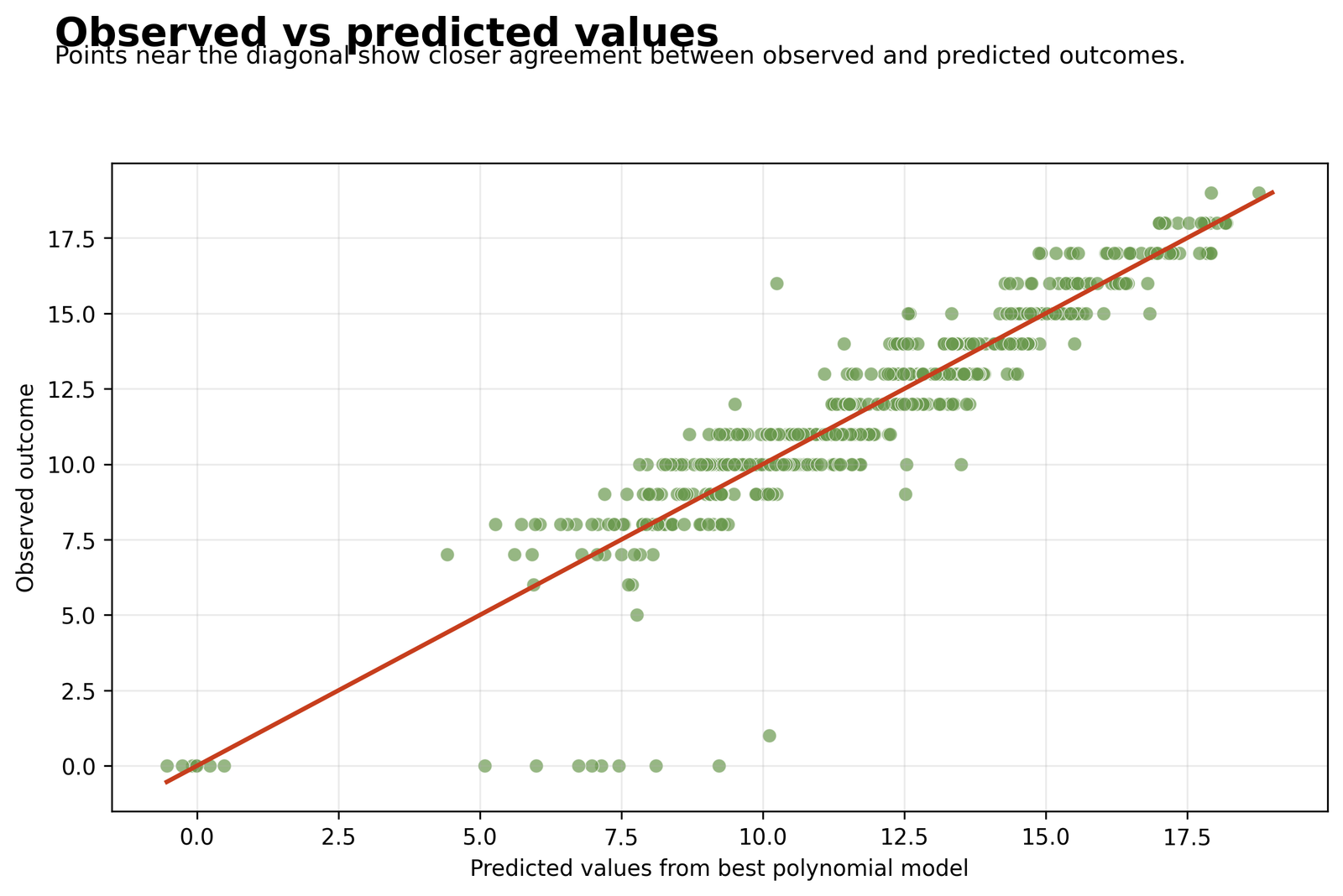
Most observations follow the diagonal from the middle to the upper outcome range. Horizontal bands appear because G3 is recorded as integer grades. Several zero outcomes sit far below their predicted values.
The selected cubic model uses 649 observations, has R² = 0.854512, adjusted R² = 0.851767, RMSE = 1.231316, and MAE = 0.763130.
The model predicts ordinary grade outcomes closely and explains about 85.45% of observed variation. The largest errors are concentrated among students with G3 = 0 whose earlier grades and covariates imply much higher fitted outcomes.
A strong overall R² does not mean every case is predicted accurately. The chart identifies the outcome region in which the model is least reliable.
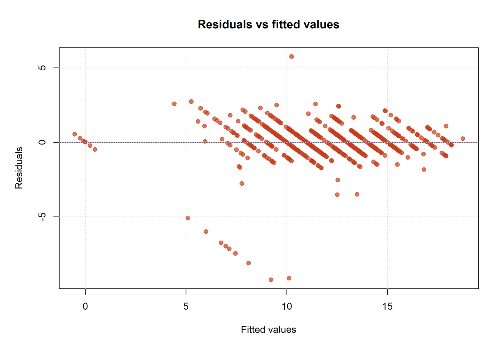
Chart 4: Residuals Versus Fitted Values
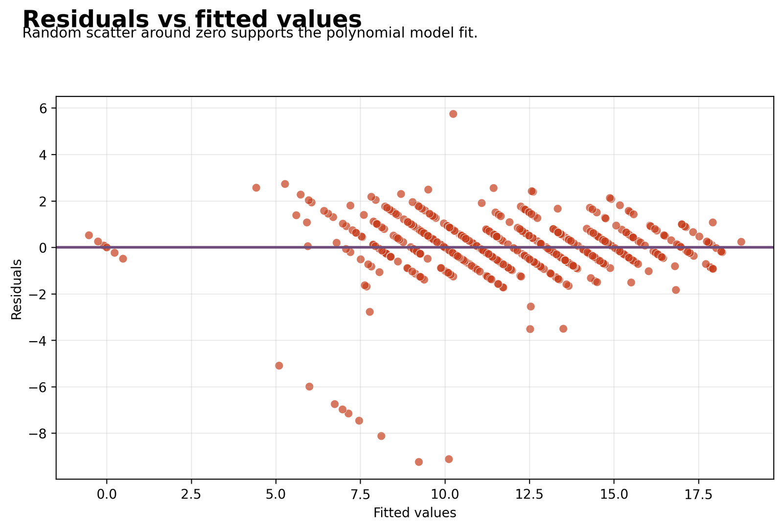
The main residual cloud is centered near zero and shows repeated downward diagonal bands caused by the integer outcome. The negative tail is longer than the positive tail, with several large overpredictions for zero outcomes.
Most residuals lie approximately between −2 and +2.5. The most negative values approach −9, while the largest positive value is approximately +5.7. Overall RMSE is 1.2313.
There is no strong remaining smooth curve through the central residual cloud, suggesting that the polynomial mean function captures the main G2 pattern. The diagonal bands are a consequence of discrete G3 values, while the long negative tail reflects unusual low outcomes rather than a universal fit failure.
Residual review is essential before accepting a curved model. Supporting diagnostics include Studentized Residuals, Cook’s Distance, and Outlier Detection.
Chart 5: Best-Model Coefficients with 95% Confidence Intervals
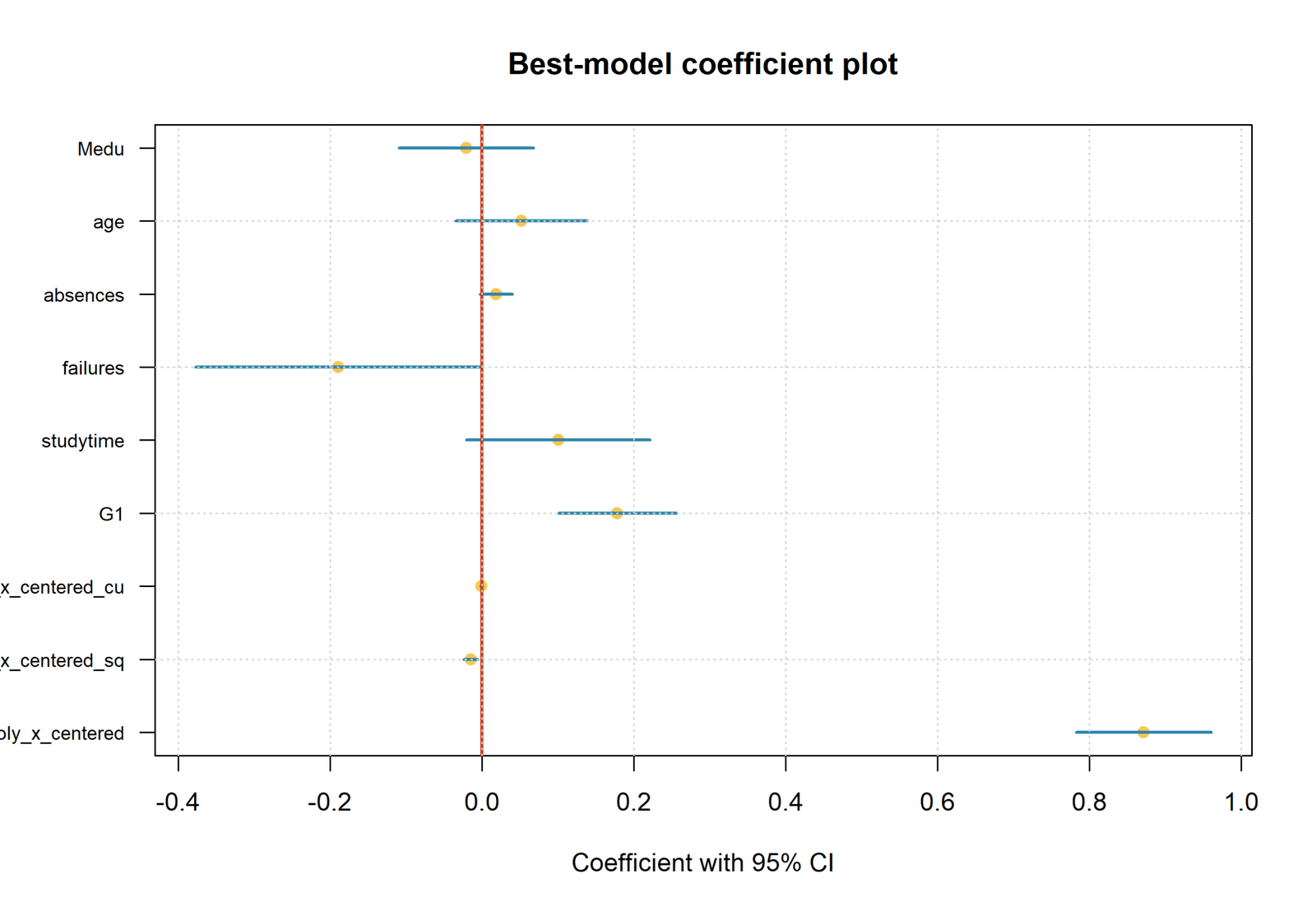
The centered linear G2 term is the largest positive coefficient. G1 is also positive and precise. The squared G2 term is negative and its interval remains below zero. Most remaining covariate intervals overlap zero.
Centered G2 B = 0.866080, p < .001; squared G2 B = −0.015395, p = .00125; cubic G2 B = −0.000710, p = .22117; G1 B = 0.183682, p < .001. Failures B = −0.187130, p = .05115.
The positive first-order term and negative squared term describe a rising relationship that gradually flattens. The cubic term does not have strong evidence after the lower-order terms and covariates are included. Coefficients for polynomial powers should be interpreted jointly rather than as separate independent effects.
This plot prevents readers from treating the degree label as the result. The substantive result is the complete fitted curve and the joint behavior of its polynomial terms.
R Charts and Explanations
The R visual sequence covers the fitted curve, model-degree comparison, prediction agreement, residual structure, and best-model coefficients. The interpretation uses the same 649-row worked analysis.
R Polynomial Curve
The R curve rises across the observed G2 range and shows only mild flattening at high values. The central relationship is strongly positive, while uncertainty grows toward the endpoints where fewer observations define the curve.
R Model Fit Comparison
Adding the quadratic term produces the meaningful improvement. The cubic model has the highest adjusted R-squared and lowest RMSE by a narrow margin, but the quadratic model has lower AIC and MAE.
R Observed Versus Predicted Values
Most cases lie close to the agreement line, supporting strong predictive fit. The major deviations involve zero or unusually low G3 outcomes that receive midrange fitted values.
R Residuals Versus Fitted Values
Residuals are broadly centered around zero without a remaining curved band. The integer outcome produces diagonal stripes, and the negative tail reflects a small group of severe overpredictions.
R Coefficient Plot
The centered G2 term and G1 are positive, the squared G2 term is negative, and the cubic term remains close to zero. Most control-variable intervals overlap zero.
Polynomial Regression Coefficient Interpretation
Cubic model coefficient table
| Term | B | SE | t | p | 95% CI | Interpretation |
|---|---|---|---|---|---|---|
| Intercept | 8.912921 | 0.947716 | 9.4046 | <.001 | 7.051890–10.773951 | Expected G3 when centered G2 = 0 and all covariates equal zero; mainly a model constant |
| Centered G2 | 0.866080 | 0.045720 | 18.9433 | <.001 | 0.776301–0.955860 | Slope of the curve at mean G2, conditional on other terms |
| Centered G2² | −0.015395 | 0.004749 | −3.2418 | .00125 | −0.024721 to −0.006070 | Negative curvature that gradually reduces the positive slope |
| Centered G2³ | −0.000710 | 0.000580 | −1.2246 | .22117 | −0.001849–0.000429 | No strong evidence that third-degree flexibility is required |
| G1 | 0.183682 | 0.039530 | 4.6467 | <.001 | 0.106057–0.261307 | Positive adjusted contribution from first-period grade |
| studytime | 0.097088 | 0.061581 | 1.5766 | .11539 | −0.023839–0.218016 | Positive but uncertain adjusted association |
| failures | −0.187130 | 0.095773 | −1.9539 | .05115 | −0.375200–0.000941 | Near-threshold negative adjusted association |
| absences | 0.017730 | 0.010969 | 1.6163 | .10652 | −0.003810–0.039271 | Small uncertain positive coefficient |
| age | 0.054082 | 0.044164 | 1.2246 | .22118 | −0.032642–0.140806 | No strong adjusted evidence |
| Medu | −0.015295 | 0.058420 | −0.2618 | .79356 | −0.130014–0.099425 | Near-zero adjusted estimate |
| Fedu | 0.016131 | 0.059131 | 0.2728 | .78510 | −0.099985–0.132247 | Near-zero adjusted estimate |
| traveltime | 0.079634 | 0.068325 | 1.1655 | .24424 | −0.054535–0.213803 | Uncertain positive coefficient |
| health | −0.061239 | 0.034301 | −1.7853 | .07469 | −0.128596–0.006119 | Negative tendency with interval crossing zero |
The centered G2 coefficient is the slope specifically at mean G2. At other G2 values, the slope combines the first-, second-, and third-degree terms. It is therefore incorrect to say that every one-point G2 increase raises G3 by exactly 0.866 points.
The squared term is statistically supported and negative, which means the curve bends downward relative to a straight line. The cubic term is not supported at α = .05. Hierarchical modeling requires the lower-order terms to remain when cubic is included.
Predictions, Slopes and Curve Shape
Predicted G3 at mean covariates
- G2 = 0 → approximately 1.05
- G2 = 5 → approximately 5.88
- G2 = 10 → approximately 10.64
- G2 = 11.57 → approximately 12.03
- G2 = 15 → approximately 14.79
- G2 = 19 → approximately 17.32
Curve interpretation
- The fitted relationship is increasing across the observed range.
- The slope is strongest through low and middle G2 values.
- The negative squared term creates gentle flattening.
- The cubic term does not create a supported turning point inside the observed range.
- Confidence is greatest near the center of the data.
At mean G2, the instantaneous slope is approximately 0.866 because the centered squared and cubic contributions to the derivative are zero. Away from the mean, the negative squared term reduces that slope. The relationship nevertheless remains positive from the observed minimum to maximum.
The derivative equation has stationary points outside the observed centered G2 interval. That means the fitted cubic curve has no estimated peak or trough within G2 values from 0 to 19. Describing the curve as strongly increasing with mild flattening is more accurate than describing it as an S-shaped relationship.
The prediction calculator in the worked workbook uses the cubic coefficients. At all input means, it returns predicted G3 of approximately 12.0302. Scenario calculations are useful for interpretation, but they should remain inside realistic combinations of predictors.
Polynomial Regression Assumptions and Diagnostics
Main checks
- Functional form and selected degree
- Residual variance
- Residual distribution
- Influential observations
- Multicollinearity among polynomial powers
- Validation and extrapolation
Current findings
- Quadratic curvature is supported
- Cubic improvement is minimal
- Central residual cloud is reasonably centered
- Zero outcomes create a long negative tail
- Prediction is strong inside the observed range
Functional Form
The purpose of Polynomial Regression is to improve functional form, but choosing a degree does not guarantee that the curve is correct. Compare candidate curves visually and consider Ramsey RESET Test logic, partial-residual plots, splines, and theory. A generalized additive model may be preferable when the shape is unknown and sufficient data are available.
Multicollinearity Among Powers
Raw X, X², and X³ can be strongly correlated. Centering reduces nonessential multicollinearity but does not make polynomial terms independent. Use Variance Inflation Factor, Tolerance Statistic, and Multicollinearity Check for diagnostic context. Orthogonal polynomial bases can improve numerical stability when individual raw-power coefficients are not the main reporting target.
Homoskedasticity
Residual variance should remain reasonably stable across fitted values. The supplied plot does not show a dominant expanding funnel in the main cloud, but formal checks such as Breusch-Pagan Test and White Test can supplement visual review. Robust standard errors may be used when the mean function is retained but variance is misspecified.
Residual Distribution
Normal residuals are most relevant for classical confidence intervals and tests, not for unbiased point prediction. The negative tail caused by zero outcomes should be described. A Q-Q Plot Normality Check can show whether tail departures are severe.
Influence and Boundary Cases
Polynomial curves are especially sensitive to predictor-boundary observations because high powers give extreme X values greater leverage over shape. Review Studentized Residuals, Cook’s Distance, and Outlier Detection before accepting a curve that changes sharply near an endpoint.
Independence
Ordinary Polynomial Regression assumes independent observations. Repeated or clustered measurements require appropriate covariance methods, fixed effects, mixed effects, or generalized estimating equations.
Validation
Degree selection should occur inside cross-validation or the training sample. Reusing the test sample to select degree and report performance creates optimistic error estimates. In machine learning, the polynomial feature step must be included inside the validation pipeline.
Polynomial Regression in Python, R, SPSS and Excel
Python Polynomial Regression
Python can create centered powers explicitly with pandas or generate features with scikit-learn. Statsmodels provides coefficient tables and inferential output; scikit-learn provides pipelines and validation tools.
- Center G2 before powers are created
- Fit linear, quadratic and cubic candidates
- Compare adjusted R², AIC, RMSE and validation error
- Plot the fitted curve and residuals
Polynomial Regression in R
R can use explicit terms such as I(z^2) and I(z^3), or poly() for raw or orthogonal polynomial bases. Use raw = TRUE when coefficients must correspond to ordinary powers.
lm()fits the modelanova()compares nested degreesAIC()andBIC()compare fit penaltiespredict()generates curves and intervals
SPSS Polynomial Regression
SPSS uses COMPUTE commands to center the predictor and create squared and cubic terms, followed by the REGRESSION procedure. Hierarchical blocks can show the incremental contribution of each degree.
- Create centered G2
- Create squared and cubed centered terms
- Enter lower-order terms before higher-order terms
- Save predicted values and residuals
Polynomial Regression in Excel
Excel can create centered powers, fit models with the Data Analysis Regression tool or matrix formulas, calculate predictions, and build a Polynomial Regression calculator.
- Center G2 with an absolute mean reference
- Create squared and cubic columns
- Use one regression column per term
- Calculate fitted values and residuals with formulas
Code: Expand Only the Software You Need
Python Polynomial Regression with statsmodels
import pandas as pd
import statsmodels.formula.api as smf

df = pd.read_csv("dataset.csv")
g2_mean = df["G2"].mean()

df["g2_c"] = df["G2"] - g2_mean
df["g2_c2"] = df["g2_c"] ** 2
df["g2_c3"] = df["g2_c"] ** 3

controls = (
    "G1 + studytime + failures + absences + age + "
    "Medu + Fedu + traveltime + health"
)

linear = smf.ols(f"G3 ~ g2_c + {controls}", data=df).fit()
quadratic = smf.ols(
    f"G3 ~ g2_c + g2_c2 + {controls}", data=df
).fit()
cubic = smf.ols(
    f"G3 ~ g2_c + g2_c2 + g2_c3 + {controls}", data=df
).fit()

print(linear.summary())
print(quadratic.summary())
print(cubic.summary())

comparison = pd.DataFrame({
    "Model": ["Linear", "Quadratic", "Cubic"],
    "R2": [linear.rsquared, quadratic.rsquared, cubic.rsquared],
    "Adjusted_R2": [
        linear.rsquared_adj,
        quadratic.rsquared_adj,
        cubic.rsquared_adj
    ],
    "AIC": [linear.aic, quadratic.aic, cubic.aic],
    "BIC": [linear.bic, quadratic.bic, cubic.bic]
})
print(comparison)
Python Polynomial Regression with scikit-learn
from sklearn.compose import ColumnTransformer
from sklearn.linear_model import LinearRegression
from sklearn.metrics import mean_squared_error
from sklearn.model_selection import KFold, cross_val_score
from sklearn.pipeline import Pipeline
from sklearn.preprocessing import PolynomialFeatures, StandardScaler

X = df[["G2"]]
y = df["G3"]

pipeline = Pipeline([
    ("poly", PolynomialFeatures(degree=3, include_bias=False)),
    ("scale", StandardScaler()),
    ("model", LinearRegression())
])

cv = KFold(n_splits=5, shuffle=True, random_state=42)
rmse = -cross_val_score(
    pipeline,
    X,
    y,
    cv=cv,
    scoring="neg_root_mean_squared_error"
)

print("Mean CV RMSE:", rmse.mean())
R Polynomial Regression code
df <- read.csv("dataset.csv")

g2_mean <- mean(df$G2, na.rm = TRUE)
df$g2_c <- df$G2 - g2_mean

linear <- lm(
  G3 ~ g2_c + G1 + studytime + failures + absences +
    age + Medu + Fedu + traveltime + health,
  data = df
)

quadratic <- lm(
  G3 ~ g2_c + I(g2_c^2) + G1 + studytime + failures +
    absences + age + Medu + Fedu + traveltime + health,
  data = df
)

cubic <- lm(
  G3 ~ g2_c + I(g2_c^2) + I(g2_c^3) + G1 +
    studytime + failures + absences + age + Medu +
    Fedu + traveltime + health,
  data = df
)

summary(cubic)
anova(linear, quadratic, cubic)
AIC(linear, quadratic, cubic)
BIC(linear, quadratic, cubic)
SPSS Polynomial Regression syntax
DESCRIPTIVES VARIABLES=G2 /SAVE.

* Replace the constant below with the sample G2 mean.
COMPUTE G2_C = G2 - 11.5701078582.
COMPUTE G2_C2 = G2_C ** 2.
COMPUTE G2_C3 = G2_C ** 3.
EXECUTE.

REGRESSION
 /DEPENDENT G3
 /METHOD=ENTER G2_C G1 studytime failures absences age
  Medu Fedu traveltime health
 /METHOD=ENTER G2_C2
 /METHOD=ENTER G2_C3
 /STATISTICS COEFF OUTS R ANOVA CHANGE CI(95)
 /SAVE PRED RESID.

OUTPUT EXPORT
 /CONTENTS EXPORT=ALL LAYERS=PRINTSETTING MODELVIEWS=PRINTSETTING
 /PDF DOCUMENTFILE=
'D:\DATA ANALYSIS\H Regression Tests and Models\Polynomial Regression\SPSS_Output\pdf\Polynomial-Regression-SPSS-Output.pdf'.
Excel Polynomial Regression formulas
Centered G2:
=B2-$B$652

Squared centered G2:
=L2^2

Cubed centered G2:
=L2^3

Cubic prediction:
=$B$4
 + L2*$B$5
 + M2*$B$6
 + N2*$B$7
 + C2*$B$8
 + D2*$B$9
 + E2*$B$10
 + F2*$B$11
 + G2*$B$12
 + H2*$B$13
 + I2*$B$14
 + J2*$B$15
 + K2*$B$16

Residual:
=Observed_G3-Predicted_G3

RMSE:
=SQRT(AVERAGE(Squared_Residual_Range))
Advanced Polynomial Regression Topics
Polynomial Regression Explained for Beginners
Polynomial Regression adds powers of a numeric predictor to a linear equation. The purpose is to let the fitted line bend while retaining ordinary regression estimation.
Steps to Perform Polynomial Regression
Inspect the scatterplot, center the predictor, create candidate powers, fit a limited degree range, compare fit and validation, inspect residuals, and report the complete curve.
Polynomial Regression Formula
A degree-d model contains X, X², and every required power through Xᵈ. Lower-order terms remain in the equation whenever a higher-order term is included.
What Degree Means
The degree is the highest predictor power in the equation. Degree one is linear, degree two is quadratic, and degree three is cubic.
How to Choose the Degree
Use theory, adjusted R², AIC, BIC, nested comparisons, residual patterns, cross-validation, and parsimony. Do not select degree solely from training R².
Linear and Polynomial Regression
A linear model forces one constant slope. Polynomial Regression allows the slope to change with X while remaining linear in the fitted coefficients.
Quadratic Polynomial Regression
A quadratic model has one curvature term and can represent a U-shaped, inverted-U, or monotonic flattening relationship depending on coefficients and the observed range.
Cubic Polynomial Regression
A cubic model adds another change in curvature. It should be retained only when the added flexibility improves prediction or answers a substantively meaningful question.
Centering Polynomial Predictors
Centering improves coefficient interpretation and reduces avoidable numerical dependence among raw powers. It does not alter the fitted curve.
Standardizing Polynomial Predictors
Standardization can help numerical stability and machine-learning pipelines. Coefficients then use standard-deviation units and require different interpretation.
Raw Versus Orthogonal Polynomials
Raw powers are easy to translate into an explicit equation. Orthogonal polynomials reduce correlation among basis terms but their individual coefficients are less directly interpretable.
Polynomial Regression Coefficients
Individual coefficients control the complete curve jointly. Use predicted values, derivatives, and graphs rather than treating each power as an isolated real-world variable.
Turning Points
Turning points occur where the derivative equals zero. A mathematical root outside the observed predictor range should not be reported as an observed peak or trough.
Marginal Effects
The marginal effect is the derivative of the fitted curve. It changes with X, so a polynomial model does not have one constant slope.
Polynomial Regression Calculator
A calculator evaluates a fixed equation for supplied inputs. It does not select degree, diagnose residuals, or protect against extrapolation.
Polynomial Regression in Machine Learning
Generate polynomial features inside a pipeline, tune degree within cross-validation, and evaluate on untouched data. Regularization becomes important as the feature set grows.
Sklearn Polynomial Regression
Scikit-learn combines PolynomialFeatures with a linear estimator. Feature generation, scaling, and model tuning should remain inside one pipeline.
Polynomial Regression in R
Use explicit I(x^2) terms for raw powers or poly() for raw or orthogonal bases. The choice affects coefficients but can represent the same fitted subspace.
Polynomial Regression in Excel
Create centered, squared, and cubic columns, then fit them as separate predictors. Excel is also useful for a transparent scenario calculator.
Polynomial Logistic Regression
Polynomial logistic regression is logistic regression containing polynomial predictor terms. It models a binary probability and is not the same as the continuous-outcome model in this article.
Polynomial Regression Assumptions
The method inherits linear-model assumptions about the conditional mean, independence, variance, residual inference, and influential observations.
Multicollinearity in Polynomial Models
Polynomial powers are naturally related. Centering, orthogonal bases, Variance Inflation Factor, and stability checks help separate harmless construction from serious numerical instability.
Overfitting
A high-degree polynomial can memorize the training sample and oscillate between observations. Validation error and visual plausibility are essential safeguards.
Extrapolation
Polynomial terms grow rapidly outside the data range. Predictions should remain inside or close to the observed range unless strong theory supports the function.
Polynomial Regression Versus Splines
Splines and Generalized Additive Model approaches provide local flexibility and often behave better than one global high-degree polynomial.
Reporting Polynomial Regression
Report centering, degree candidates, selection criterion, full coefficient hierarchy, fit statistics, predicted curves, residual findings, and the observed predictor range.
APA-Style Reporting
The cubic model had the highest adjusted R², R² = .855, adjusted R² = .852, RMSE = 1.231, and MAE = 0.763. The quadratic model had the lowest AIC, AIC = 2137.40, compared with 2137.87 for the cubic model.
In the cubic specification, the centered linear G2 term was positive, B = 0.866, SE = 0.046, t = 18.943, p < .001, 95% CI [0.776, 0.956]. The squared term was negative, B = −0.0154, SE = 0.0047, t = −3.242, p = .001, 95% CI [−0.0247, −0.0061], indicating mild flattening. The cubic term was not statistically significant, B = −0.00071, SE = 0.00058, t = −1.225, p = .221.
The fitted relationship remained increasing throughout the observed G2 range. Model comparison therefore supported curvature, but the cubic term added little beyond the quadratic form.
Publication Checklist
Include
- Outcome and polynomial predictor
- Centering or scaling constant
- Every candidate degree
- Selection criterion
- Lower-order hierarchy
- R², adjusted R², AIC, BIC, RMSE and MAE
- Curve with confidence band
- Residual and influence checks
- Observed predictor range
- Software and reproducible code
Avoid
- Selecting a high degree from R² alone
- Removing lower-order terms
- Interpreting squared and cubic coefficients separately
- Calling the method nonlinear in its coefficients
- Ignoring boundary leverage
- Extrapolating far beyond the data
- Reporting one curve without alternatives
- Claiming causation from fitted curvature
Use Confidence Interval, P-Value, Effect Size, and Statistical Power terminology only where it matches the fitted analysis and research design.
Downloads and Chart Resources
Polynomial Regression CurveFitted cubic curve and 95% confidence band
Model Fit ComparisonAdjusted R² and RMSE across linear, quadratic, and cubic models
Observed Versus PredictedAgreement plot for the selected polynomial model
Residual DiagnosticResiduals versus fitted values
Coefficient PlotBest-model coefficients and 95% confidence intervals
Frequently Asked Questions
What is Polynomial Regression?
Polynomial Regression is a linear regression model that adds powers of a numeric predictor so the fitted response can follow a curved path.
When should Polynomial Regression be used?
Use it when theory or diagnostics indicate smooth curvature and a limited-degree polynomial is plausible across the observed predictor range.
Is Polynomial Regression linear or nonlinear?
It is nonlinear in the predictor but linear in its coefficients, so ordinary least squares can estimate it.
What is the Polynomial Regression formula?
A quadratic model is Y = β0 + β1X + β2X² + ε. A cubic model adds β3X³. Covariates can be included in the same equation.
What does polynomial degree mean?
Degree is the highest predictor power. Degree one is linear, degree two is quadratic, and degree three is cubic.
How do I choose the degree?
Compare a small theory-driven set using validation, adjusted R², AIC, BIC, residuals, and parsimony. Avoid selecting degree from training R² alone.
Why center the predictor?
Centering improves interpretation and numerical stability. It does not change the fitted curve or predictions.
How do I interpret Polynomial Regression coefficients?
Interpret the powers jointly. Use the fitted curve, derivative, predicted values, and turning points rather than isolated coefficient effects.
What is the best model in this example?
Cubic has the highest adjusted R² and lowest RMSE. Quadratic has the lowest AIC and MAE, and the cubic term is not significant, so quadratic is more parsimonious.
What does the negative squared term mean?
It makes the positive G2 slope gradually smaller as G2 increases, producing mild flattening.
Does the curve have a turning point in the observed range?
No. The fitted cubic relationship remains increasing for observed G2 values from 0 to 19.
How is Polynomial Regression different from nonlinear regression?
Polynomial Regression is linear in its coefficients. Nonlinear regression contains parameters that enter the mean function nonlinearly.
How is Polynomial Regression used in Python?
Create polynomial features explicitly or with scikit-learn, fit a linear estimator, and select degree within a validation pipeline.
How is Polynomial Regression fitted in R?
Use lm() with I(x^2) and I(x^3), or use poly() for raw or orthogonal polynomial bases.
How do I perform Polynomial Regression in Excel?
Create centered, squared, and cubic columns, include them as regression predictors, and calculate fitted values with the estimated coefficients.
What is polynomial logistic regression?
It is logistic regression with polynomial predictor terms for a binary outcome. It is different from the continuous-outcome Polynomial Regression model used here.
Polynomial Regression Conclusion
Polynomial Regression extends straight-line regression when a predictor has a smooth curved relationship with a continuous outcome. The model remains linear in its coefficients, but squared and cubic predictor terms allow its slope to change across the observed range.
In this 649-observation analysis, G3 rises strongly with G2. The negative squared term indicates mild flattening at higher G2 values. The cubic model has the highest adjusted R² and lowest RMSE, but the quadratic model has lower AIC and MAE, and the cubic term is not statistically significant.
The appropriate substantive conclusion is therefore stronger than “cubic is best” and more accurate than “the relationship is linear.” The data support a curved, monotonically increasing relationship, while the third-degree term contributes very little beyond the quadratic form.

