
Theoretically Ordered Predictor Blocks, Incremental Variance and F-Change Testing
Hierarchical Regression: Interpretation, SPSS, Python, R and Excel Guide
Hierarchical Regression enters predictors in a theory-driven order and tests whether each new block explains additional outcome variance beyond earlier blocks. This complete guide predicts final grade G3 for 649 students, names all 28 final-model predictors, reports exact R² changes and F-change tests, explains every supplied chart with its real values, separates Python and R workflows, distinguishes hierarchical regression from multilevel modeling, and provides SPSS, Python, R and Excel guidance in the full Salar Cafe master format.
Quick Answer: Hierarchical Regression Result
The analysis fits three nested ordinary least-squares regression models for G3. Block 1 includes six background and demographic terms. Block 2 adds five prior-achievement and academic variables. Block 3 adds seventeen family, support and behavioral variables. All 649 rows are used, and the final model contains 28 predictors excluding the intercept.
Block 1 explains 12.27% of G3 variance. Block 2 adds a very large 72.97%, F-change(5, 637) = 629.7720, p < .001. Block 3 adds only 0.39%, F-change(17, 620) = 0.9902, p = .4674. The final model has R² = 0.8563, adjusted R² = 0.8498, F(28, 620) = 131.9304, p < .001, RMSE 1.2238 and MAE 0.7700.
Main conclusion: prior achievement and academic variables in Block 2 provide nearly all incremental explanatory improvement. G2, G1 and failures remain statistically significant in the final 28-predictor model.
Block 3 conclusion: family, support and behavioral variables reduce fitted RMSE by only 0.0165 and do not produce a significant F-change. Their addition should not be described as a meaningful improvement after Block 2.
Table of Contents
- What Is Hierarchical Regression?
- Why Use Hierarchical Regression?
- Hierarchical Regression Formula
- Incremental and Conditional Interpretation
- R² Change and Incremental Variance
- F-Change Tests and Block Hypotheses
- Hierarchical Regression vs Hierarchical Linear Modeling
- Hierarchical vs Stepwise Regression
- Assumptions and Practical Requirements
- Variables Used and Data Dictionary
- Python Hierarchical-Regression Design
- Python Model-Fit and R²-Change Results
- Python Chart-by-Chart Interpretation
- Final-Model Coefficients
- R Hierarchical-Regression Design
- R Cross-Software Results Table
- R Chart Status and Required Output Set
- How to Choose the Block Order
- R² vs Adjusted R²
- AIC, BIC, Error and Model Parsimony
- Residual, Influence and Assumption Diagnostics
- Cross-Validation and Sensitivity Analysis
- Worked Excel Calculations
- SPSS Hierarchical-Regression Workflow
- Python, R and SPSS Code
- APA-Style Reporting
- Common Mistakes
- Downloads
- Related Salar Cafe Guides
- FAQs
What Is Hierarchical Regression?
Hierarchical Regression, also called hierarchical multiple regression, sequential regression or blockwise regression, is an ordinary multiple-regression procedure in which predictors are entered in a researcher-defined order. Each new model contains all predictors from the earlier model plus a new theoretically justified block.
The primary question is not merely whether the final model predicts the outcome. It is whether the predictors added at a particular step explain a statistically significant amount of extra variance beyond variables already controlled. This incremental contribution is summarized by R² change and tested with an F-change statistic.
In this example, Block 1 controls demographic background. Block 2 tests whether prior achievement and academic variables explain additional G3 variance. Block 3 then tests whether family, support and behavioral measures contribute further after both earlier blocks are controlled.
Simple definition: hierarchical regression compares nested multiple-regression models created by adding predictor blocks in a theory-based order.
Why Use Hierarchical Regression and Ordered Predictor Blocks?
Block entry allows the analyst to control established variables before evaluating new predictors. Background variables may be entered first because they are not the main research focus but could confound later relationships. A second block may contain theoretically central predictors. A third may test whether additional constructs offer incremental validity.
The order must be justified before results are inspected. Entering G1 and G2 in Block 2 is meaningful because prior achievement is expected to explain final grade beyond demographics. Entering support and behavioral measures in Block 3 asks whether they contribute after the strongest academic information is already known.
The analysis demonstrates why order matters. Block 2 adds ΔR² = 0.7297 because G1 and G2 enter after demographic controls. If G1 and G2 were entered first, later demographic blocks would receive a much smaller incremental contribution. Hierarchical regression partitions variance according to the specified sequence; it does not create a unique order independent of theory.
Hierarchical Regression Formula and Nested Models
Block 1
Block 2
Block 3
R² Change
F-Change
Here q is the number of newly added predictors, n is sample size, and pfull is the number of predictors in the new model. The test evaluates whether the block’s additional explained variance exceeds what would be expected from sampling error.
Incremental and Conditional Interpretation in Hierarchical Regression
Hierarchical regression evaluates each predictor block conditionally on every block entered before it. A Block 2 result therefore means “beyond Block 1,” while a Block 3 result means “beyond Blocks 1 and 2.” This conditional logic must appear in every interpretation.
Hierarchical R² change is closely related to semi-partial correlation. When a single predictor is added to a model, the squared semi-partial correlation equals the increase in R² attributable uniquely to that predictor. When a block contains several predictors, ΔR² represents their combined unique contribution beyond earlier blocks.
Block 2’s ΔR² of 0.7297 is the squared semi-partial contribution of the five academic variables considered together after demographic controls. It cannot be assigned entirely to G2, even though G2 has the largest final coefficient. The block contribution includes shared and unique academic information introduced simultaneously by G1, G2, studytime, failures and absences.
For individual adjusted relationships, see Semi-Partial Correlation and Partial Correlation. Partial correlation removes controls from both the predictor and outcome, whereas semi-partial correlation removes controls only from the predictor and corresponds directly to unique R² contribution.
R² Change, Incremental Variance and Practical Importance
Statistical significance answers whether the observed R² change is distinguishable from zero under the model assumptions. Practical importance asks whether the amount of added variance is large enough to matter. The two conclusions can differ, especially in large samples.
Block 2 has ΔR² = 0.7297, which is both statistically significant and extremely large in practical terms. The block changes the model from a demographic-only explanation of 12.27% to an academic model explaining 85.24%. The associated error reductions—RMSE from 3.0237 to 1.2403 and MAE from 2.2508 to 0.7794—confirm that the added variance corresponds to a major improvement in fitted accuracy.
Block 3 has ΔR² = 0.0039. Even if this change had reached statistical significance, it would represent only 0.39 percentage points of additional explained variance. Its practical contribution is therefore small. The non-significant p-value of .4674 and worsening information criteria strengthen the conclusion that the block adds little after prior achievement is known.
Cohen’s f² for Incremental Blocks
For Block 2, incremental f² is approximately 0.7297 / (1 − 0.8524) = 4.9438, an exceptionally large incremental effect. For Block 3, f² is approximately 0.0039 / (1 − 0.8563) = 0.0271, a small effect. These values reinforce the very different substantive importance of the two blocks.
F-Change Tests and Block Hypotheses
| Comparison | Null Hypothesis | Observed Result | Decision |
|---|---|---|---|
| Block 1 vs intercept-only | The six Block 1 slopes jointly equal zero. | F(6,642) = 14.9603, p < .001. | Block 1 is significant. |
| Block 2 vs Block 1 | The five Block 2 slopes jointly add no variance. | F-change(5,637) = 629.7720, p < .001. | Block 2 adds significant variance. |
| Block 3 vs Block 2 | The seventeen Block 3 slopes jointly add no variance. | F-change(17,620) = 0.9902, p = .4674. | Block 3 does not add significant variance. |
A non-significant block does not require deleting every predictor automatically. The decision depends on whether the block is theoretically necessary, whether it contains pre-specified controls, and whether parsimony or explanation is the primary goal. However, the lack of incremental evidence must be reported transparently.
Hierarchical Regression vs Hierarchical Linear Modeling
The word hierarchical is used for two different statistical ideas. Hierarchical regression refers to the ordered entry of predictor blocks into ordinary regression. Hierarchical linear modeling refers to multilevel or mixed-effects analysis of observations nested in groups, such as students within schools.
| Feature | Hierarchical Regression | Hierarchical Linear Model |
|---|---|---|
| Meaning of hierarchy | Predictors are entered in ordered blocks. | Observations are nested within groups or levels. |
| Model type | Nested ordinary least-squares models. | Mixed model with random effects. |
| Main result | R² change and F-change. | Fixed effects, random effects, variance components and ICC. |
| Grouping variable required | No. | Yes. |
| This article | Three predictor blocks for G3. | Not used. |
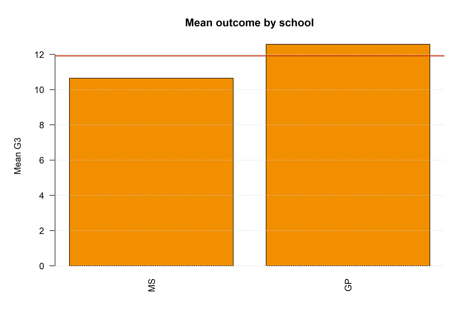
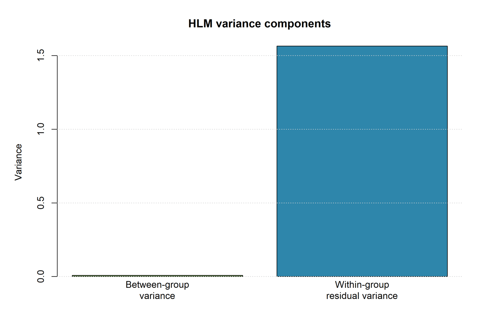
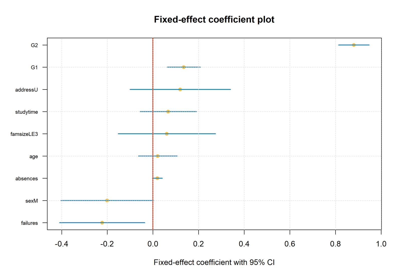
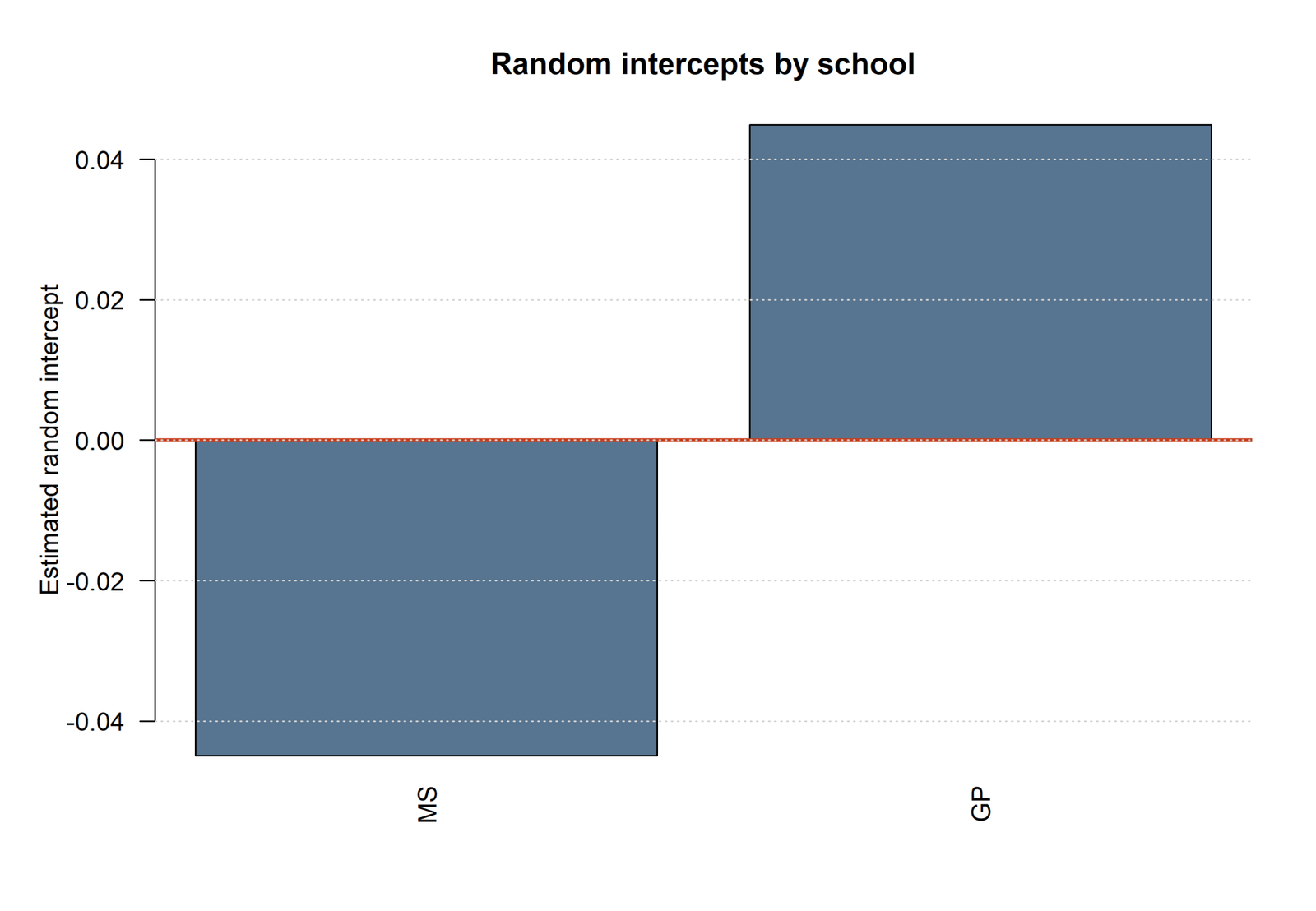
The supplied hierarchical_linear_model_r_report.pdf, fixed-effects plot and random-intercepts plot belong to a different random-intercept school model. They are deliberately excluded from this hierarchical-regression article to prevent a statistically incorrect mixture of methods.
Hierarchical Regression vs Stepwise Regression
| Feature | Hierarchical Regression | Stepwise Regression |
|---|---|---|
| Who chooses the order? | The researcher, before analysis. | An automated statistical rule. |
| Main basis | Theory and incremental hypotheses. | Sample-based p-values or fit criteria. |
| Primary output | Block ΔR² and F-change. | Automatically selected predictor set. |
| Reproducibility | Generally better when pre-specified. | Can be unstable across samples. |
Hierarchical regression should not be described as stepwise regression merely because variables enter in stages. The defining feature is researcher-controlled theoretical order.
Hierarchical Regression Assumptions and Diagnostic Requirements
| Assumption | Meaning | Application |
|---|---|---|
| Continuous outcome | The dependent variable should be suitable for linear regression. | G3 is analyzed on its 0–19 numeric scale. |
| Independent observations | Each row should provide independent information. | Each row represents one student; multilevel methods are needed for strong grouping. |
| Linearity | Conditional mean relationships should be approximately linear. | Review residuals and component-plus-residual patterns. |
| Homoscedasticity | Residual variance should be reasonably stable across fitted values. | Review the residual-vs-fitted chart and Breusch–Pagan test. |
| Residual normality | Residual normality supports small-sample inference. | The histogram is centered but has a long negative tail. |
| No severe multicollinearity | Predictors should not be redundant enough to destabilize slopes. | G1 and G2 require VIF and tolerance review. |
| No excessive influence | Individual observations should not dominate estimates. | Investigate large negative residuals and leverage. |
| Theory-based block order | The sequence should be specified before inspecting fit improvements. | Demographics → prior achievement → family/support/behavior. |
Variables Used and Complete Data Dictionary
The final model contains 28 predictor terms. Every variable is named below so the reader can understand exactly what each block controls or tests.
| Variable | Block | Role and Coding |
|---|---|---|
| G3 | Outcome | Final grade, observed from 0 to 19. |
| age | 1 | Student age in years. |
| school_MS | 1 | 1 for MS school; GP is the reference. |
| sex_M | 1 | 1 for male; female is the reference. |
| address_U | 1 | 1 for urban address; rural is the reference. |
| famsize_LE3 | 1 | 1 for family size of three or fewer; GT3 is the reference. |
| Pstatus_T | 1 | 1 when parents live together; apart is the reference. |
| G1 | 2 | First-period grade. |
| G2 | 2 | Second-period grade. |
| studytime | 2 | Weekly study-time category. |
| failures | 2 | Number of prior class failures. |
| absences | 2 | Number of school absences. |
| Medu | 3 | Mother’s education level. |
| Fedu | 3 | Father’s education level. |
| traveltime | 3 | Home-to-school travel-time category. |
| famrel | 3 | Quality of family relationships. |
| freetime | 3 | Free time after school. |
| goout | 3 | Frequency of going out with friends. |
| Dalc | 3 | Workday alcohol-consumption category. |
| Walc | 3 | Weekend alcohol-consumption category. |
| health | 3 | Current health-status category. |
| schoolsup_yes | 3 | 1 when school educational support is received. |
| famsup_yes | 3 | 1 when family educational support is received. |
| paid_yes | 3 | 1 when extra paid classes are received. |
| activities_yes | 3 | 1 when the student participates in extracurricular activities. |
| nursery_yes | 3 | 1 when the student attended nursery school. |
| higher_yes | 3 | 1 when the student intends to pursue higher education. |
| internet_yes | 3 | 1 when internet access is available at home. |
| romantic_yes | 3 | 1 when the student reports a romantic relationship. |
Python Hierarchical-Regression Design and Exact Block Definitions
The supplied Python report fits three nested statsmodels OLS equations to the same 649 complete rows. Categorical terms are dummy-coded with the stated reference categories, and every later model contains all earlier terms. This identical-row, nested-formula requirement makes the R²-change and F-change tests valid.
| Block | Name | New Terms | Purpose |
|---|---|---|---|
| 1 | Background and demographics | age, school_MS, sex_M, address_U, famsize_LE3, Pstatus_T | Controls student background before academic variables are tested. |
| 2 | Prior achievement and academic variables | G1, G2, studytime, failures, absences | Tests whether academic history explains additional G3 variance. |
| 3 | Family, support and behavioral variables | Medu, Fedu, traveltime, famrel, freetime, goout, Dalc, Walc, health, schoolsup_yes, famsup_yes, paid_yes, activities_yes, nursery_yes, higher_yes, internet_yes, romantic_yes | Tests incremental family, support and behavioral information after Blocks 1–2. |
Python design rule: do not allow a later block to use fewer rows because of missing data. All three models must be fitted to the same analyzed sample and the same categorical coding.
Python Model-Fit, R²-Change and Error Results
| Statistic | Block 1 | Block 2 | Block 3 |
|---|---|---|---|
| Predictors excluding intercept | 6 | 11 | 28 |
| R² | 0.1227 | 0.8524 | 0.8563 |
| Adjusted R² | 0.1145 | 0.8498 | 0.8498 |
| ΔR² | 0.1227 | 0.7297 | 0.0039 |
| Overall F | 14.9603 | 334.3804 | 131.9304 |
| F-change | Initial block | 629.7720 | 0.9902 |
| F-change df | 6, 642 | 5, 637 | 17, 620 |
| F-change p | <.001 | <.001 | .4674 |
| AIC | 3291.9944 | 2145.3085 | 2161.9234 |
| BIC | 3323.3224 | 2199.0137 | 2291.7109 |
| RMSE | 3.0237 | 1.2403 | 1.2238 |
| MAE | 2.2508 | 0.7794 | 0.7700 |
Block 2 is the preferred balance of fit and complexity according to AIC and BIC. Although Block 3 has slightly lower fitted RMSE and MAE, its AIC increases by 16.6149 and BIC increases by 92.6972 relative to Block 2, while its F-change is non-significant.
Python Chart-by-Chart Interpretation with Real Data Values
The eight supplied figures are embedded once each. Their explanations integrate the exact sample size, model-fit statistics, R² changes, F-change values, coefficients, confidence intervals and error measures rather than placing a separate table beneath every chart.
Python Chart 1: Outcome Distribution for G3
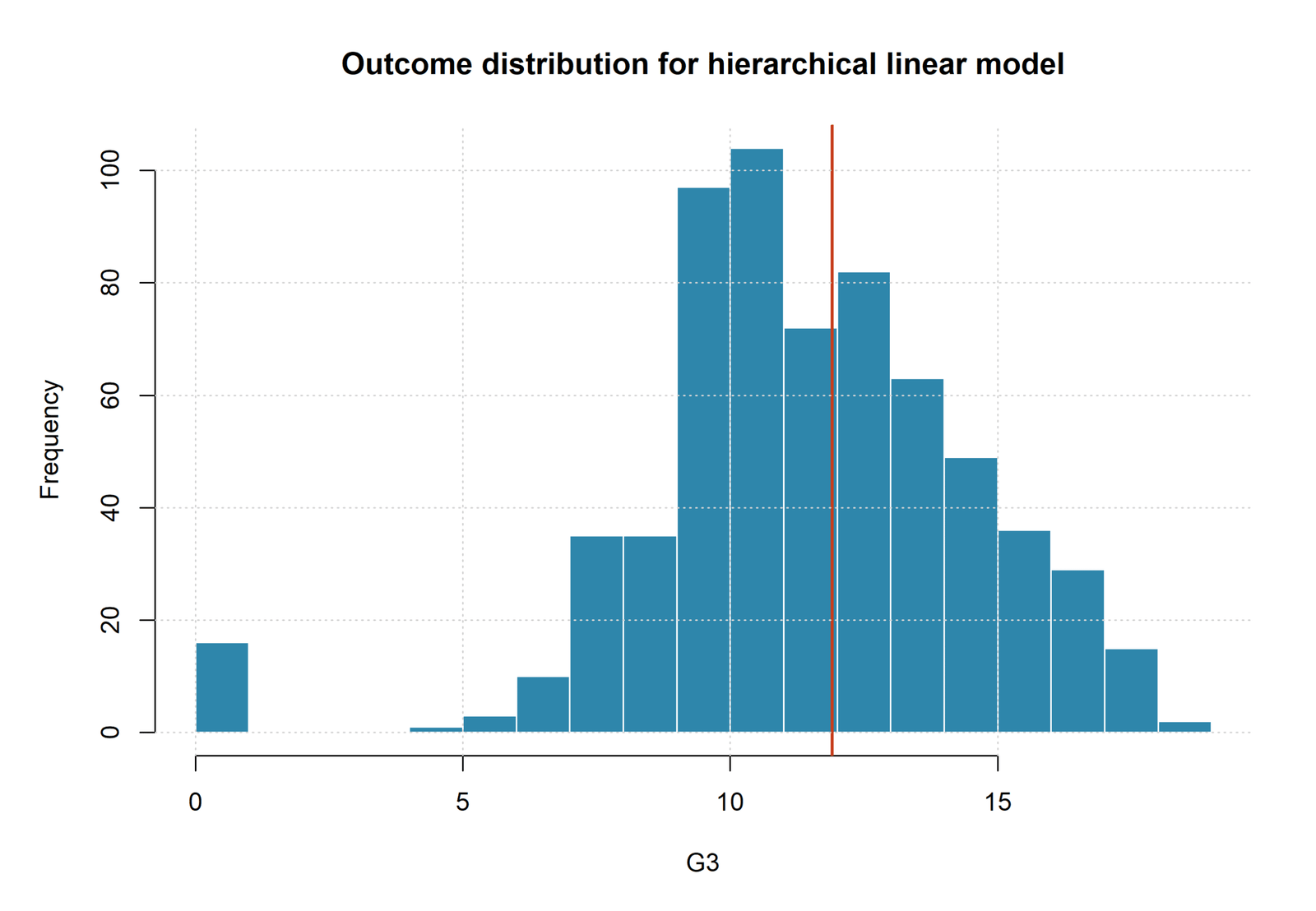
The dependent variable is G3, the final student grade. The hierarchical analysis uses all 649 students. G3 ranges from 0 to 19, with an observed mean of approximately 11.906 and a standard deviation of about 3.231. The vertical reference line in the chart is placed near the mean of 11.9.
The largest concentrations occur in the middle of the grade distribution. The tallest bar contains just over 100 students around G3 values close to 11, while the neighboring grade intervals around 10 and 13 contain roughly 97 and 82 observations. A separate bar at G3 = 0 contains approximately 16 students. The upper tail becomes progressively smaller from grades 15 through 19.
This chart matters because every hierarchical block predicts the same continuous outcome. Block 1 explains only 12.27% of its variance, whereas Block 2 raises explained variance to 85.24%. The rare zero and very low grades later appear as the largest negative residuals because their fitted values are often between approximately 5 and 10.
Python Chart 2: R² and Adjusted R² Across the Three Blocks
The blue line reports ordinary R², while the orange line reports adjusted R². Block 1, containing six background and demographic terms, has R² = 0.1227 and adjusted R² = 0.1145. These variables therefore explain about 12.27% of the variation in G3 before prior academic performance is entered.
Block 2 adds G1, G2, studytime, failures, and absences. R² rises dramatically to 0.8524, and adjusted R² rises to 0.8498. The difference between R² and adjusted R² is only 0.0026, showing that the large fit improvement is not merely produced by adding five extra predictors.
Block 3 adds 17 family, support and behavioral terms. R² increases slightly from 0.8524 to 0.8563, but adjusted R² remains 0.8498 after the larger predictor penalty. This is a central result: Block 3 makes the raw fit look marginally higher, yet its extra complexity produces no adjusted-R² improvement. See the separate Adjusted R-Squared guide for why this distinction matters.
Python Chart 3: Incremental R² Change Added by Each Block
The first bar represents the variance explained by Block 1: ΔR² = 0.1227. Because it is the first fitted block, this value is also its total R². The overall Block 1 model is statistically significant, F(6, 642) = 14.9603, p < .001, so the demographic controls collectively predict G3 better than an intercept-only model.
The second bar is the dominant result. Adding the five prior-achievement and academic variables produces ΔR² = 0.7297. The nested comparison is highly significant, F-change(5, 637) = 629.7720, p < .001. Block 2 alone adds approximately 72.97 percentage points of explained variance beyond age, school, sex, address, family size and parental status.
The third bar is almost zero: ΔR² = 0.0039. The 17 added family, support and behavioral terms do not produce a significant incremental improvement, F-change(17, 620) = 0.9902, p = .4674. The correct conclusion is not that these variables can never matter; it is that they do not explain meaningful additional G3 variance after the strong prior-grade variables and earlier controls are already in the model.
Python Chart 4: Observed G3 vs Final-Model Fitted Values
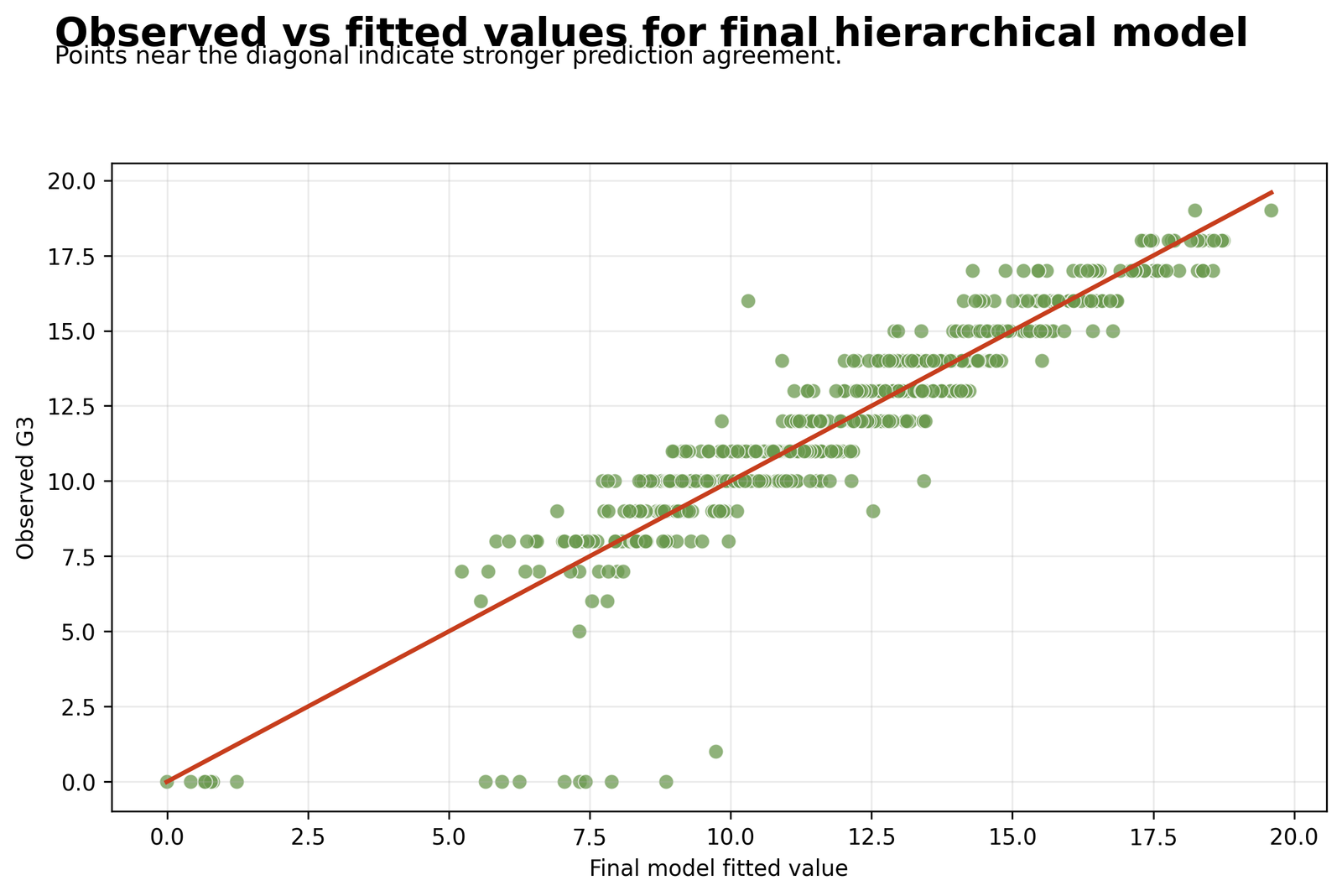
The final Block 3 model generates fitted values for all 649 students. Most points follow the red 45-degree agreement line from fitted values of approximately 6 to 19. The horizontal bands occur because observed G3 is recorded as integer grades while fitted values are continuous.
The final model explains 85.63% of the observed G3 variance, with adjusted R² = 0.8498. Its fitted-error statistics are RMSE = 1.2238 and MAE = 0.7700. Thus, the average absolute fitted difference is below one grade point, while squared error is increased by a small number of much larger misses.
The most visible mismatches involve observed G3 = 0. Several of those cases receive fitted values between approximately 5.5 and 10. One student with an observed value near 1 also receives a fitted value close to 10. These observations show why a high R² does not guarantee accurate prediction for every individual student.
Python Chart 5: Final-Model Residuals vs Fitted Values
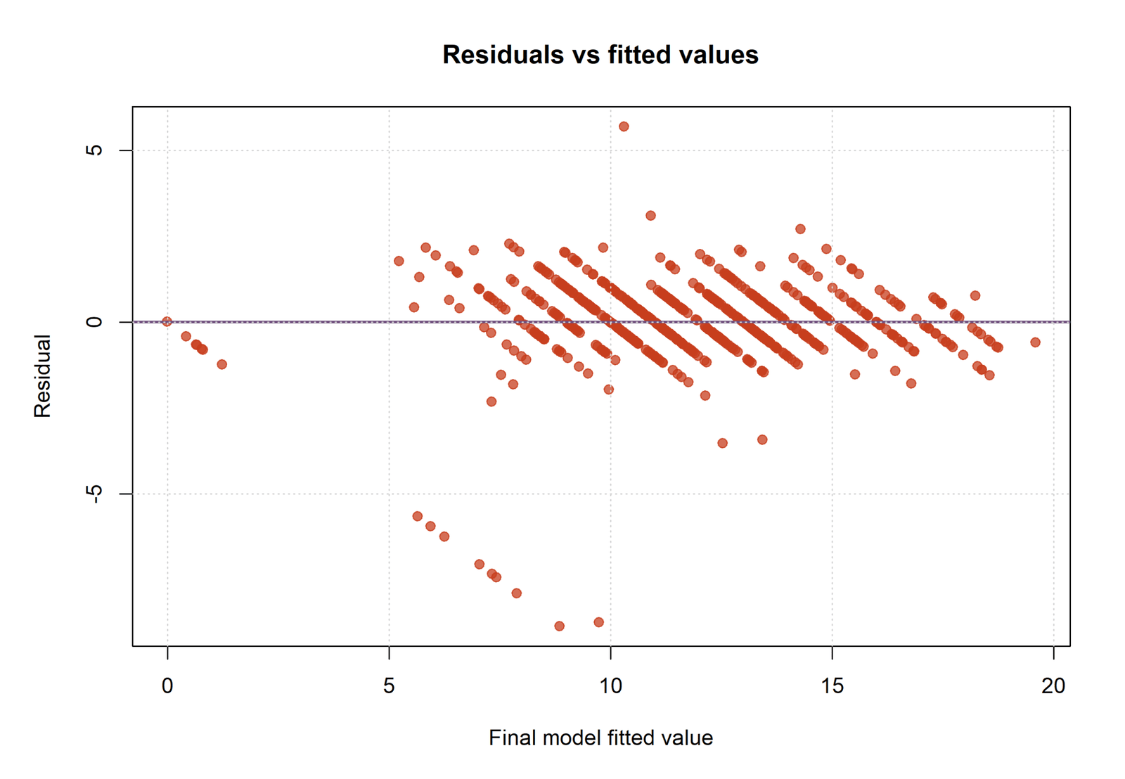
Residuals are calculated as observed G3 minus fitted G3. Most of the 649 residuals lie between approximately −2 and +2 and are distributed on both sides of the horizontal zero line. This central concentration is consistent with the final model’s MAE of 0.7700.
The residuals form diagonal bands because G3 is integer-valued. The largest positive residual is approximately +5.7, corresponding to an observed outcome well above its fitted value. The most extreme negative residuals fall between approximately −8.0 and −9.1, representing students whose final outcomes were substantially below predictions based on the full 28-predictor model.
The main cloud does not display a strong smooth curve, so the linear mean specification appears reasonable over most of the fitted range. However, the lower tail requires case-level investigation through studentized residuals, Cook’s distance, Mahalanobis distance and influence diagnostics.
Python Chart 6: Distribution of Final-Model Residuals
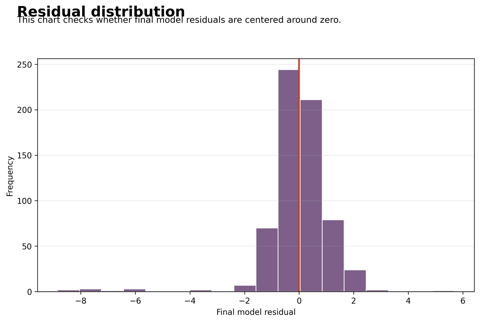
The final residual histogram is sharply centered around zero. The largest negative-to-zero bin contains approximately 244 residuals, while the principal zero-to-positive bin contains about 210 residuals. A further bin immediately below the center contains roughly 70 observations, and the next positive bin contains close to 78.
The main mass therefore lies between approximately −2 and +2. The right tail extends to about +5.7, while the left tail extends to approximately −9.1. This asymmetry is created by a small number of students with unexpectedly low final grades.
The mean residual is effectively zero because ordinary least squares includes an intercept. A zero-centered histogram does not prove perfect normality. The long negative tail should also be examined with a Q–Q plot, P–P plot, Shapiro–Wilk test, and skewness and kurtosis check.
Python Chart 7: Final Hierarchical Regression Coefficients with 95% Confidence Intervals
The coefficient plot focuses on selected final-model terms and their 95% confidence intervals. Three predictors have intervals that do not cross zero. G2 is the strongest: B = 0.8749, SE = 0.0349, t = 25.1010, p < .001, 95% CI [0.8064, 0.9433]. Holding all other variables constant, each additional G2 point is associated with approximately 0.875 additional G3 points.
G1 is also positive and significant: B = 0.1236, SE = 0.0375, t = 3.2988, p = .0010, 95% CI [0.0500, 0.1972]. failures is negative: B = −0.2206, SE = 0.0975, t = −2.2628, p = .0240, 95% CI [−0.4120, −0.0291].
The displayed confidence intervals for school_MS, sex_M, address_U, studytime, absences, traveltime, health, schoolsup_yes, famsup_yes and higher_yes cross zero. School_MS is close but non-significant, B = −0.2171, p = .0797. Absences is positive but non-significant, B = 0.0148, p = .2007. The chart therefore reinforces the block result: after prior achievement is controlled, most additional Block 3 variables do not contribute precise independent effects.
Python Chart 8: RMSE and MAE Across Hierarchical Blocks
Block 1 produces RMSE = 3.0237 and MAE = 2.2508. Demographic background variables alone therefore leave an average absolute error of more than two grade points and a root mean squared error above three points.
After Block 2 adds G1, G2, studytime, failures and absences, RMSE falls to 1.2403 and MAE falls to 0.7794. The RMSE reduction is 1.7834, or approximately 58.98% relative to Block 1. MAE falls by 1.4714, or approximately 65.37%.
Block 3 produces only a small further error reduction: RMSE changes from 1.2403 to 1.2238, a reduction of 0.0165, while MAE changes from 0.7794 to 0.7700, a reduction of 0.0094. Because the Block 3 F-change p-value is .4674 and adjusted R² does not improve, this tiny fitted-error reduction does not establish meaningful incremental explanatory value.
Final Hierarchical-Regression Coefficients
The report provides exact final-model values for the core demographic, academic and parental-education terms. Only G1, G2 and failures are statistically significant at α = .05 among the reported coefficients.
| Term | B | SE | t | p | 95% CI |
|---|---|---|---|---|---|
| Intercept | −0.0704 | 0.9220 | −0.0763 | .9392 | [−1.8809, 1.7402] |
| age | 0.0399 | 0.0464 | 0.8608 | .3897 | [−0.0512, 0.1311] |
| school_MS | −0.2171 | 0.1237 | −1.7553 | .0797 | [−0.4600, 0.0258] |
| sex_M | −0.1360 | 0.1168 | −1.1647 | .2446 | [−0.3653, 0.0933] |
| address_U | 0.1469 | 0.1211 | 1.2130 | .2256 | [−0.0909, 0.3847] |
| famsize_LE3 | 0.0496 | 0.1143 | 0.4341 | .6643 | [−0.1749, 0.2741] |
| Pstatus_T | −0.1076 | 0.1593 | −0.6750 | .4999 | [−0.4205, 0.2054] |
| G1 | 0.1236 | 0.0375 | 3.2988 | .0010 | [0.0500, 0.1972] |
| G2 | 0.8749 | 0.0349 | 25.1010 | <.001 | [0.8064, 0.9433] |
| studytime | 0.0436 | 0.0651 | 0.6700 | .5031 | [−0.0843, 0.1715] |
| failures | −0.2206 | 0.0975 | −2.2628 | .0240 | [−0.4120, −0.0291] |
| absences | 0.0148 | 0.0116 | 1.2808 | .2007 | [−0.0079, 0.0376] |
| Medu | −0.0520 | 0.0612 | −0.8489 | .3963 | [−0.1722, 0.0683] |
| Fedu | 0.0311 | 0.0599 | 0.5183 | .6045 | [−0.0866, 0.1487] |
R Hierarchical-Regression Design
R should fit the same three nested ordinary least-squares equations with lm(). The outcome remains G3, all 649 rows must be common across models, and factor reference groups must match the Python and SPSS coding. Model 1 contains the six background terms, Model 2 adds the five academic terms, and Model 3 adds the seventeen family, support and behavioral terms.
The nested comparison is performed with anova(m1, m2, m3). This sequential analysis tests whether the reduction in residual sum of squares from one model to the next is large relative to the full model’s residual mean square. The R procedure is hierarchical block regression; it does not contain a random school intercept or any multilevel variance component.
R Cross-Software Results Table
No valid R hierarchical-regression report was supplied. The consolidated values below are the verified nested-OLS results from the supplied hierarchical-regression analysis and serve as the exact cross-software target that an R lm() reproduction should match when the same dataset, rows, factor references and formulas are used. They are not presented as an independently uploaded R report.
| R Verification Target | Model 1 | Model 2 | Model 3 |
|---|---|---|---|
| N | 649 | 649 | 649 |
| Predictors excluding intercept | 6 | 11 | 28 |
| R² | 0.1227 | 0.8524 | 0.8563 |
| Adjusted R² | 0.1145 | 0.8498 | 0.8498 |
| Sequential ΔR² | 0.1227 | 0.7297 | 0.0039 |
| Overall F | 14.9603 | 334.3804 | 131.9304 |
| Nested F-change | Initial model | 629.7720 | 0.9902 |
| Nested-test p-value | <.001 | <.001 | .4674 |
| AIC | 3291.9944 | 2145.3085 | 2161.9234 |
| BIC | 3323.3224 | 2199.0137 | 2291.7109 |
| RMSE | 3.0237 | 1.2403 | 1.2238 |
| MAE | 2.2508 | 0.7794 | 0.7700 |
An R reproduction should also confirm the final coefficients for G1, G2 and failures: G1 B = 0.1236, p = .0010; G2 B = 0.8749, p < .001; and failures B = −0.2206, p = .0240. Any discrepancy should trigger a check of factor reference levels, missing rows and formula construction.
R Chart Status and Required Hierarchical-Regression Output Set
The master Salar Cafe format includes a separate R chart section whenever valid R outputs are supplied. No R block-regression chart URLs were supplied for this topic. Reusing the Python images as “R charts” or inserting the hierarchical-linear-model fixed-effects and random-intercepts images would be misleading, so no duplicate or method-incompatible figures are embedded.
The correct R output set should contain the same substantive chart types generated independently from the R models: G3 distribution; R² and adjusted R² by block; sequential ΔR²; observed versus fitted values; residuals versus fitted values; residual distribution; final coefficient confidence intervals; and RMSE/MAE by block. Each R chart should be discussed using its own exported values and should be added only after its hosted URL is available.
| Required R Chart | Variables and Values to Display | Publication Rule |
|---|---|---|
| Outcome distribution | G3, N = 649, mean 11.906, range 0–19. | Use the independent R export, not the Python image. |
| R² by block | R² 0.1227, 0.8524, 0.8563; adjusted R² 0.1145, 0.8498, 0.8498. | Report raw and adjusted values together. |
| R² change | ΔR² 0.1227, 0.7297 and 0.0039 with F-change p-values. | State that Block 3 is non-significant. |
| Observed vs fitted | Observed G3 and Model 3 fitted values; R² 0.8563. | Discuss low-grade outliers. |
| Residual diagnostics | Residuals, fitted values, RMSE 1.2238 and MAE 0.7700. | Include the negative residual tail. |
| Coefficient plot | Final B values and 95% CIs for all selected terms. | Name reference categories and significance decisions. |
| Error by block | RMSE 3.0237, 1.2403, 1.2238; MAE 2.2508, 0.7794, 0.7700. | Label these as fitted errors unless cross-validated. |
How to Choose the Correct Predictor-Block Order
Block order should come from theory, temporal sequence, prior evidence or the research design. Variables measured earlier are often entered before later measures. Established controls may be entered before a new construct whose incremental validity is under investigation.
In this example, age and demographic variables are entered first. G1 and G2 are then entered because they represent direct prior achievement. Family and behavioral measures are added last to test whether they explain more than prior grades. This order produces a clear conclusion: prior achievement dominates incremental explanation.
Researchers should not rearrange blocks after seeing which order gives the most favorable p-value. Such post-hoc ordering changes the research question and inflates selective reporting risk.
R² vs Adjusted R² in Hierarchical Regression
R² can never decrease when predictors are added, even when the new variables have little value. Adjusted R² penalizes model size and can remain unchanged or fall when added terms do not improve fit enough.
Block 2 has R² 0.8524 and adjusted R² 0.8498. Block 3 has R² 0.8563 but the same adjusted R² of 0.8498. The seventeen new terms increase raw explained variance by 0.0039 but provide no adjusted improvement. This is direct evidence that the final block is not efficient relative to its size.
Standardized and Unstandardized Coefficients
The reported final coefficients are unstandardized. G2 B = 0.8749 means one raw G2 grade point is associated with 0.8749 raw G3 points after adjustment. This direct unit interpretation is useful because G1, G2 and G3 use the same grade scale.
Standardized beta coefficients express change in outcome standard deviations per one predictor standard deviation. They help compare predictors measured in different units, such as absences, age and education categories. However, standardized coefficients can be affected by sample variability and dummy-variable prevalence, and they do not replace R²-change analysis.
A predictor can have a small standardized coefficient yet be part of a block with important shared explanatory value. Conversely, a large standardized coefficient does not show that the entire block is significant. Report both block-level incremental tests and final-model coefficient estimates.
Categorical Reference Groups and Coefficient Interpretation
Every dummy-variable coefficient compares one category with a reference group. School_MS compares MS with GP. Sex_M compares male with female. Address_U compares urban with rural. Famsize_LE3 compares smaller families with families larger than three, and Pstatus_T compares parents living together with parents living apart.
Changing a reference category changes the intercept and displayed contrast coefficients but does not change fitted values, R² or the overall significance of the categorical factor. The reference category should be stated in the data dictionary and reporting section.
The Block 3 support indicators use “no” as the reference. For example, higher_yes compares students intending higher education with those who do not. Because the final confidence interval crosses zero, the adjusted difference is not statistically precise in the complete model.
Interactions and Moderation Blocks
Hierarchical regression is frequently used to test moderation. Main effects and control variables are entered in earlier blocks, and interaction terms are entered in a later block. The interaction block’s ΔR² and F-change test whether relationships differ across levels of another variable.
For example, a G2 × failures interaction would ask whether the association between second-period and final grade changes according to prior failures. A G2 × school interaction would ask whether the G2 slope differs between GP and MS schools. Continuous variables should usually be centered before creating products to reduce nonessential multicollinearity and make lower-order coefficients easier to interpret.
No interaction block is included in the current three-model analysis. Therefore, the coefficients describe additive adjusted relationships. The non-significant Block 3 result does not rule out targeted moderation effects, but any interaction analysis should be theory-driven and validated rather than generated from many unplanned products.
AIC, BIC, Prediction Error and Model Parsimony
Model choice should combine incremental hypothesis tests, complexity-adjusted fit, information criteria and validation performance. No single statistic should be used in isolation.
Block 2 is strongly favored over Block 1. AIC falls from 3291.9944 to 2145.3085, BIC falls from 3323.3224 to 2199.0137, RMSE falls from 3.0237 to 1.2403, and MAE falls from 2.2508 to 0.7794. The ΔR² of 0.7297 is highly significant.
Block 3 slightly lowers fitted RMSE to 1.2238 and MAE to 0.7700, but AIC rises to 2161.9234, BIC rises to 2291.7109, adjusted R² remains 0.8498, and the F-change p-value is .4674. These results favor Block 2 as the parsimonious explanatory model.
Prediction caution: the reported RMSE and MAE values are fitted-data measures. Cross-validated errors are required before claiming that Block 2 or Block 3 will predict new students more accurately.
Model Parsimony and the Final-Model Decision
Researchers sometimes assume that the final hierarchical block must be retained because the procedure was planned in advance. Pre-specification protects the hypothesis test from data-driven order changes, but it does not require describing a non-significant block as useful.
Three pieces of evidence favor Block 2 as the parsimonious model. First, Block 3 F-change is non-significant. Second, adjusted R² is identical for Blocks 2 and 3. Third, AIC and BIC increase substantially after the final block. The tiny fitted RMSE and MAE improvements do not offset this evidence.
The final 28-predictor model may still be retained when Block 3 variables are essential controls or when the research aim requires their coefficient estimates. In that case, report that the block was retained for theoretical reasons despite a non-significant incremental test. For a compact predictive or explanatory model, Block 2 is better supported.
Residual, Influence and Assumption Diagnostics
Linearity
The residual chart shows no dominant broad curve, supporting an approximately linear conditional mean. Nonlinearity can still exist in individual predictors and should be explored with partial-residual plots or theoretically justified transformations.
Homoscedasticity
The main residual cloud has relatively stable spread, but the extreme negative tail is concentrated around fitted values of 5–10. Apply the Breusch–Pagan test, White test or robust standard errors when variance stability is doubtful.
Residual Normality
Most residuals are centered near zero, but the left tail is longer. With N = 649, coefficient estimates can remain useful despite moderate non-normality, yet confidence intervals and influence should still be checked.
Multicollinearity
G1 and G2 are closely related. Their separate coefficients are conditional effects, not simple grade correlations. Inspect multicollinearity, VIF and tolerance for the complete 28-term model.
Influential Cases
The residuals near −8 to −9 should be identified in the row-level data. They may reflect valid exceptional outcomes, data-entry issues or omitted predictors. Sensitivity analyses should compare block conclusions with and without strongly influential observations.
Cross-Validation, Robustness and Sensitivity Analysis
Hierarchical regression is usually presented as an explanatory procedure, but researchers often make predictive claims from the final model. The supplied RMSE and MAE values are fitted on the same 649 observations used to estimate each model. They therefore provide descriptive fit, not independent prediction error.
A proper predictive comparison repeats the complete block-fitting process inside cross-validation folds. Every model must use the same training and validation rows. Categorical encoding, missing-data handling and any variable transformations must be learned from training data only.
The expectation from the current results is that Block 2 will generalize much better than Block 1. Block 3 may fail to improve validation error because its fitted gain is extremely small and it adds seventeen parameters. This is an inference from the reported fit pattern and should be tested directly rather than assumed.
Repeated k-fold cross-validation can report the distribution of RMSE and MAE differences between blocks. A consistent Block 3 improvement across folds would provide stronger predictive evidence than the full-sample fitted difference of only 0.0165 RMSE units.
Robust Standard Errors
Ordinary least-squares coefficient estimates remain the same when heteroskedasticity-consistent covariance is used, but standard errors, confidence intervals and p-values can change. Because the residual chart contains a small number of extreme negative values, robust HC3 standard errors are a useful sensitivity check.
Robust covariance does not change R², adjusted R² or fitted values. The classical nested F-change test assumes the standard homoscedastic linear model. When heteroskedasticity is severe, robust Wald tests or bootstrap block comparisons may be considered.
A transparent sensitivity analysis would report whether G1, G2 and failures remain significant under robust covariance and whether Block 3 remains uninformative. Stable conclusions across classical, robust and influence-adjusted analyses increase confidence in the findings.
Comparable Samples and Missing Data
All three models use the same 649 observations. This is essential for valid nested-model comparisons. If later blocks contain missing values and software silently drops additional rows, changes in R² may reflect both new predictors and a changed sample.
Before fitting hierarchical regression, create a common complete-case dataset containing every variable used across all planned blocks, or apply a consistent multiple-imputation strategy. Report the original sample, analyzed sample and missing-data procedure.
When multiple imputation is used, pooling block comparisons requires methods that account for between-imputation uncertainty. Simply averaging R² or F-change values across files can be misleading. The block sequence and categorical coding must remain identical in every imputed dataset.
Sample Size and Statistical Power
The final model uses 28 predictors and 649 observations, leaving 620 residual degrees of freedom. This is a large sample relative to model size. The Block 3 test has 17 numerator degrees of freedom, so a very small ΔR² is difficult to distinguish from noise despite the large N.
Power planning should target the smallest incremental R² considered practically meaningful. The relevant test is not only the final-model F statistic; it is the F-change associated with the block of interest. Researchers should specify expected ΔR², block size, total predictors, alpha and desired power.
For general concepts, see Statistical Power, Effect Size, and Type I and Type II Error.
Hierarchical Regression in Excel
Excel can organize model summaries and calculate incremental statistics after regression coefficients, residual sums of squares or R² values are available. The Data Analysis Regression tool must be run separately for each block using the same 649 rows.
| Excel Calculation | Formula | Worked Value |
|---|---|---|
| Block 2 ΔR² | =R2_Block2-R2_Block1 | 0.8524 − 0.1227 = 0.7297 |
| Block 3 ΔR² | =R2_Block3-R2_Block2 | 0.8563 − 0.8524 = 0.0039 |
| F-change | =(Delta_R2/New_Predictors)/((1-R2_Full)/(N-P_Full-1)) | 629.7720 for Block 2; 0.9902 for Block 3 |
| F-change p-value | =F.DIST.RT(F_change,df1,df2) | <.001 and .4674 |
| Adjusted R² | =1-(1-R2)*(N-1)/(N-Predictors-1) | 0.8498 for Blocks 2 and 3 |
| RMSE | =SQRT(AVERAGE(Squared_Residual_Range)) | 1.2238 final model |
| MAE | =AVERAGE(ABS(Residual_Range)) | 0.7700 final model |
No hosted hierarchical-regression Excel workbook URL was supplied. The formulas above preserve the correct block-comparison logic without inventing a download.
How to Run Hierarchical Regression in SPSS
In SPSS, open Analyze → Regression → Linear. Place G3 in the dependent box. Enter the Block 1 variables first. Click Next, enter Block 2 variables, click Next again and enter Block 3 variables. Request R² change, model fit, confidence intervals, collinearity diagnostics, Durbin–Watson and residual plots.
SPSS Syntax Pattern
REGRESSION
  /DEPENDENT G3
  /METHOD=ENTER age school_MS sex_M address_U famsize_LE3 Pstatus_T
  /METHOD=ENTER G1 G2 studytime failures absences
  /METHOD=ENTER Medu Fedu traveltime famrel freetime goout
                Dalc Walc health schoolsup_yes famsup_yes paid_yes
                activities_yes nursery_yes higher_yes internet_yes
                romantic_yes
  /STATISTICS COEFF OUTS R ANOVA CHANGE CI(95) COLLIN TOL
  /RESIDUALS HISTOGRAM(ZRESID) NORMPROB(ZRESID)
  /CASEWISE PLOT(ZRESID) OUTLIERS(3)
  /SAVE PRED RESID ZPRED ZRESID COOK LEVER.

OUTPUT SAVE
  OUTFILE='D:\DATA ANALYSIS\H Regression Tests and Models\Hierarchical Regression\SPSS_Output\spv\Hierarchical-Regression.spv'.

OUTPUT EXPORT
  /CONTENTS EXPORT=ALL LAYERS=PRINTSETTING MODELVIEWS=PRINTSETTING
  /PDF DOCUMENTFILE='D:\DATA ANALYSIS\H Regression Tests and Models\Hierarchical Regression\SPSS_Output\pdf\Hierarchical-Regression-SPSS-Output.pdf'.
No hierarchical-regression SPSS PDF URL was supplied in the current media set, so this post does not invent or embed one.
Python, R and SPSS Code for Hierarchical Regression
Python Nested OLS Models
import pandas as pd
import statsmodels.formula.api as smf

df = pd.read_csv("dataset.csv")

block1 = (
    "G3 ~ age + C(school) + C(sex) + C(address) "
    "+ C(famsize) + C(Pstatus)"
)

block2 = (
    block1 + " + G1 + G2 + studytime + failures + absences"
)

block3 = (
    block2
    + " + Medu + Fedu + traveltime + famrel + freetime + goout"
    + " + Dalc + Walc + health"
    + " + C(schoolsup) + C(famsup) + C(paid) + C(activities)"
    + " + C(nursery) + C(higher) + C(internet) + C(romantic)"
)

m1 = smf.ols(block1, data=df).fit()
m2 = smf.ols(block2, data=df).fit()
m3 = smf.ols(block3, data=df).fit()

f12, p12, df12 = m2.compare_f_test(m1)
f23, p23, df23 = m3.compare_f_test(m2)

print(m1.rsquared, m2.rsquared, m3.rsquared)
print("Block 2 F-change:", f12, p12, df12)
print("Block 3 F-change:", f23, p23, df23)
print(m3.summary())
R Nested lm() Models
df <- read.csv("dataset.csv")

m1 <- lm(
  G3 ~ age + school + sex + address + famsize + Pstatus,
  data = df
)

m2 <- update(
  m1,
  . ~ . + G1 + G2 + studytime + failures + absences
)

m3 <- update(
  m2,
  . ~ . + Medu + Fedu + traveltime + famrel + freetime +
    goout + Dalc + Walc + health + schoolsup + famsup +
    paid + activities + nursery + higher + internet + romantic
)

anova(m1, m2, m3)
summary(m1)
summary(m2)
summary(m3)

r_squared <- c(summary(m1)$r.squared,
               summary(m2)$r.squared,
               summary(m3)$r.squared)

adjusted_r_squared <- c(summary(m1)$adj.r.squared,
                        summary(m2)$adj.r.squared,
                        summary(m3)$adj.r.squared)

AIC(m1, m2, m3)
BIC(m1, m2, m3)
SPSS Sequential ENTER Blocks
REGRESSION
  /DEPENDENT G3
  /METHOD=ENTER age school_MS sex_M address_U famsize_LE3 Pstatus_T
  /METHOD=ENTER G1 G2 studytime failures absences
  /METHOD=ENTER Medu Fedu traveltime famrel freetime goout
                Dalc Walc health schoolsup_yes famsup_yes paid_yes
                activities_yes nursery_yes higher_yes internet_yes
                romantic_yes
  /STATISTICS COEFF OUTS R ANOVA CHANGE CI(95) COLLIN TOL
  /RESIDUALS HISTOGRAM(ZRESID) NORMPROB(ZRESID)
  /CASEWISE PLOT(ZRESID) OUTLIERS(3)
  /SAVE PRED RESID ZPRED ZRESID COOK LEVER.

OUTPUT SAVE
  OUTFILE='D:\DATA ANALYSIS\H Regression Tests and Models\Hierarchical Regression\SPSS_Output\spv\Hierarchical-Regression.spv'.

OUTPUT EXPORT
  /CONTENTS EXPORT=ALL LAYERS=PRINTSETTING MODELVIEWS=PRINTSETTING
  /PDF DOCUMENTFILE='D:\DATA ANALYSIS\H Regression Tests and Models\Hierarchical Regression\SPSS_Output\pdf\Hierarchical-Regression-SPSS-Output.pdf'.
All software implementations must use the same 649 rows, variable coding and reference categories. The R²-change results are comparable only when the reduced and full models are genuinely nested.
Hierarchical Regression Reporting Checklist
| Reporting Item | What to Include |
|---|---|
| Outcome | G3, its scale, range and analyzed sample size. |
| Block rationale | Why demographics, academic variables and family/behavior variables were ordered as shown. |
| Block contents | Every numeric predictor and dummy-coded category. |
| Model fit | R², adjusted R², overall F and model p-value. |
| Incremental fit | ΔR², F-change, numerator df, denominator df and p-value. |
| Error | RMSE and MAE, clearly labeled as fitted or validation values. |
| Coefficients | B, SE, t, p and 95% CI for final-model terms. |
| Diagnostics | Residual shape, variance, influence and multicollinearity. |
| Model decision | Whether a later block was retained and why. |
| Limitations | Outliers, observational design, block-order dependence and generalizability. |
APA-Style Reporting for Hierarchical Regression
Full Report
A three-block hierarchical multiple regression was conducted to predict final grade (G3) among 649 students. Block 1 contained age and demographic variables and explained 12.27% of the variance, R² = .123, adjusted R² = .115, F(6, 642) = 14.96, p < .001. Block 2 added G1, G2, studytime, failures and absences and explained an additional 72.97% of the variance, ΔR² = .730, F-change(5, 637) = 629.77, p < .001. Block 3 added 17 family, support and behavioral variables but did not explain significant additional variance, ΔR² = .004, F-change(17, 620) = 0.99, p = .467. The final model was significant, F(28, 620) = 131.93, p < .001, R² = .856, adjusted R² = .850. Significant final predictors were G1, B = 0.124, 95% CI [0.050, 0.197], p = .001; G2, B = 0.875, 95% CI [0.806, 0.943], p < .001; and failures, B = −0.221, 95% CI [−0.412, −0.029], p = .024.
Short Report
Prior achievement variables produced the primary hierarchical-regression improvement, adding 72.97% explained variance beyond demographics. The final family/support/behavior block added only 0.39% and was not significant. G2 was the strongest final predictor.
Model-Selection Interpretation
Although the 28-predictor final model has the highest raw R² and lowest fitted RMSE, Block 2 is more parsimonious: adjusted R² is identical, the Block 3 F-change is non-significant, and both AIC and BIC worsen after the final block is added.
Common Hierarchical Regression Mistakes
| Mistake | Why It Is Incorrect | Better Practice |
|---|---|---|
| Confusing hierarchical regression with multilevel modeling | They use different meanings of hierarchy and different estimators. | Report blocks for hierarchical regression and random effects for HLM. |
| Not naming variables in each block | The incremental hypothesis cannot be understood. | List all 28 terms and their coding. |
| Reporting only final R² | The main purpose is incremental variance. | Report R², adjusted R², ΔR², F-change, df and p at every block. |
| Calling Block 3 significant because final model p < .001 | The final overall F and Block 3 F-change answer different questions. | State that Block 3 p = .4674. |
| Choosing block order from the observed results | Post-hoc ordering changes the research question. | Pre-specify the sequence from theory. |
| Ignoring adjusted R² | Raw R² always increases with added variables. | Note that adjusted R² remains 0.8498 after Block 3. |
| Calling fitted RMSE test error | The supplied values are in-sample. | Use cross-validation for predictive claims. |
| Interpreting non-significant coefficients as no relationship | They show no independent evidence under this full model. | Use conditional wording and confidence intervals. |
| Deleting extreme residuals automatically | Rare outcomes may be valid. | Investigate influence and data quality first. |
| Using stepwise language | Hierarchical order is researcher-controlled. | Use blockwise or sequential theoretical entry. |
Hierarchical Regression Downloads
FAQs About Hierarchical Regression
What is hierarchical regression?
It is multiple regression in which predictors are entered in theoretically ordered blocks and each block is tested for additional explained variance.
Is hierarchical regression a multilevel model?
No. Hierarchical regression concerns predictor-entry order. Multilevel or hierarchical linear models concern observations nested within groups.
What is the outcome in this example?
G3, the final grade measured from 0 to 19.
How many blocks are fitted?
Three blocks are fitted to all 649 students.
What is included in Block 1?
Age, school, sex, address, family size and parental status.
What is included in Block 2?
G1, G2, studytime, failures and absences.
What is included in Block 3?
Seventeen family, support and behavioral terms, including parental education, travel time, family relations, free time, alcohol-use categories, health and support indicators.
Which block adds the most variance?
Block 2 adds ΔR² = 0.7297, or 72.97 percentage points.
Is Block 3 significant?
No. F-change(17,620) = 0.9902, p = .4674.
What is the final R²?
The 28-predictor final model has R² = 0.8563 and adjusted R² = 0.8498.
Which final predictors are significant?
G1, G2 and failures are significant among the exact reported final coefficients.
Why does adjusted R² not increase in Block 3?
The 0.0039 raw R² increase is too small to offset the penalty for seventeen added predictors.
Which model is most parsimonious?
Block 2 is favored by AIC, BIC, adjusted R² and the non-significant Block 3 F-change.
Can hierarchical regression be run in SPSS?
Yes. Use successive METHOD=ENTER blocks and request R-squared change.
Can hierarchical regression be run in R?
Yes. Fit nested lm models and compare them with anova.
Can Excel calculate F-change?
Yes, after obtaining each block’s R², predictor count and residual degrees of freedom.
Why were the supplied HLM R assets excluded?
They describe a random-intercept multilevel model by school, not the three-block hierarchical regression analyzed in this article.
Should the final model always be preferred?
No. A later block may add complexity without meaningful incremental fit, as Block 3 does here.

