
Part correlation, unique variance, R-squared change, residualized predictor and regression interpretation
Semi Partial Correlation: Formula, Interpretation, Python, R, SPSS and Excel Guide
Semi Partial Correlation, also called semipartial correlation or part correlation, measures the unique relationship between an outcome and the part of one predictor that is not explained by other control variables. In this worked example, the outcome is G3 final grade, the focal predictor is G2, and the controls are G1, studytime, failures and absences. The result shows that G2 makes a large and statistically significant unique contribution to G3 after the controls are already in the model.
Quick Answer: Semi Partial Correlation Result
The main analysis tested whether G2 uniquely predicts G3 after controlling for G1, studytime, failures and absences. The dataset contains 649 complete cases. Before controls, the zero-order correlation between G2 and G3 is r = 0.918548, which is a very strong positive relationship.
After removing from G2 the part explained by the controls, the semi-partial correlation between G3 and the residualized part of G2 is sr = 0.397992. The squared semi-partial correlation is sr² = 0.158397. This means that G2 uniquely explains about 15.84% additional variance in G3 after G1, studytime, failures and absences are already included.
Final interpretation: G2 makes a statistically significant unique contribution to G3 after controlling G1, studytime, failures and absences, sr = 0.398, sr² = 0.158, F change = 681.557, p < .001. The unique effect is practically meaningful because the added predictor increases R² from 0.6922 to 0.8506.
Important distinction: Partial correlation and semi-partial correlation are not the same. Partial correlation residualizes both the outcome and the focal predictor. Semi-partial correlation residualizes only the focal predictor. That is why semi-partial sr² directly equals the R² change when the focal predictor is added last in hierarchical regression.
Table of Contents
- What Is Semi Partial Correlation?
- Why Use Semi Partial Correlation?
- Semi Partial vs Partial Correlation
- Semi Partial Correlation Formula
- Null and Alternative Hypotheses
- Dataset and Variables Used
- Verified Semi Partial Correlation Results
- Reduced Model vs Full Model
- Full Model Coefficients
- Python Chart-by-Chart Interpretation
- R Chart-by-Chart Interpretation
- SPSS Output and Workflow Interpretation
- Excel Worked File Explanation
- Python, R, SPSS and Excel Workflows
- Code Blocks and Excel Formulas
- Assumptions and Diagnostics
- How to Report Semi Partial Correlation
- Common Mistakes
- Downloads and Resources
- Related Statistical Guides
- FAQs About Semi Partial Correlation
What Is Semi Partial Correlation?
Semi partial correlation measures the relationship between an outcome variable and the unique part of a predictor after that predictor has been adjusted for other variables. It is also called part correlation because it correlates the outcome with only the unique part of the focal predictor.
In this guide, the focal predictor is G2. The controls are G1, studytime, failures and absences. First, G2 is predicted from the controls. Then the leftover part of G2, called residualized G2, is correlated with G3. That correlation is the semi-partial correlation.
Semi partial correlation is closely connected to hierarchical regression. When a focal predictor is added to a model after controls, the squared semi-partial correlation equals the increase in model R². In this example, adding G2 after the controls increases R² by 0.158397. Therefore, sr² = 0.158397.
This topic connects with Correlation in Python, Correlation in R, Correlation in SPSS, Correlation in Excel, Correlation Matrix, Correlation vs Regression, Multiple Linear Regression, Regression Residual Analysis, Effect Size, p-value and Confidence Interval.
Simple definition: Semi partial correlation is the correlation between Y and the part of X that remains after X has been residualized on the control variables.
Why Use Semi Partial Correlation?
Use semi partial correlation when you want to know how much unique variance a predictor adds to an outcome after other variables are already considered. It is especially helpful in hierarchical regression, model comparison and explanatory research.
| Research Need | Why Semi Partial Correlation Helps | Example in This Guide |
|---|---|---|
| Measure unique contribution | sr² tells how much additional variance the focal predictor explains. | G2 uniquely explains 15.84% additional variance in G3. |
| Compare reduced and full models | sr² equals R² change when the focal predictor is added last. | R² increases from 0.6922 to 0.8506 after adding G2. |
| Understand predictor importance | It separates unique predictor contribution from shared predictor overlap. | G2 remains highly important even after controlling G1 and other variables. |
| Explain regression coefficients | It connects coefficient significance with unique variance explained. | G2 has t = 26.1066 and p < .001 in the full model. |
| Report effect size | sr and sr² are interpretable as correlation and unique variance. | sr = 0.398 and sr² = 0.158. |
For students and researchers, semi partial correlation is useful because it tells a different story from ordinary correlation. The zero-order G2–G3 correlation is extremely high, but semi partial correlation asks a sharper question: how much does G2 still add after G1, studytime, failures and absences are already controlled?
Semi Partial vs Partial Correlation
Partial correlation and semi partial correlation are often confused. Both use control variables, but they residualize different parts of the analysis.
| Measure | What Is Residualized? | Question Answered | Main Result Here |
|---|---|---|---|
| Zero-order correlation | Nothing | How strongly are raw G2 and raw G3 related? | r = 0.918548 |
| Partial correlation | Both G2 and G3 are residualized on controls | How strongly are the residual parts of G2 and G3 related? | partial r = 0.717325 |
| Semi partial correlation | Only G2 is residualized on controls | How strongly is G3 related to the unique part of G2? | sr = 0.397992 |
| Squared semi partial correlation | Unique part of G2 in predicting G3 | How much unique variance does G2 add? | sr² = 0.158397 |
The key practical difference is that partial r² and semi partial sr² answer different variance questions. Partial r² is about the remaining residual variance after controls. Semi partial sr² is about the total outcome variance uniquely added by the focal predictor. That makes semi partial sr² especially useful for model-change interpretation.
Reporting rule: If your goal is “unique variance added to the model,” report semi partial sr² or R² change. If your goal is “relationship between residualized X and residualized Y,” report partial correlation.
Semi Partial Correlation Formula
The residual definition of semi partial correlation is:
In this guide:
The unique variance formula is:
Using the verified model values:
Because the coefficient for G2 in the full model is positive, the semi partial correlation is positive:
The F-change test for one added predictor is:
Here, df1 = 1, df2 = 643, F change = 681.556962, and p = 5.437936e-103. In a normal report, this is written as p < .001.
Null and Alternative Hypotheses
The semi partial correlation hypothesis asks whether the focal predictor adds unique explanatory value after controls are already included.
| Statement | Hypothesis | Meaning |
|---|---|---|
| Null hypothesis | H0: sr = 0 | G2 does not add unique variance to G3 after controlling G1, studytime, failures and absences. |
| Alternative hypothesis | H1: sr ≠ 0 | G2 adds unique variance to G3 after the controls. |
| Equivalent model-change hypothesis | H0: ΔR² = 0 | Adding G2 does not improve the model. |
| Observed result | p < .001 | Reject the null hypothesis. |
Decision: G2 makes a statistically significant unique contribution to G3 after the controls are included. The result is not only statistically significant; it is also meaningful because ΔR² = 0.158397.
Dataset and Variables Used
The analysis uses the student performance dataset. The outcome is G3 final grade. The focal predictor is G2 second-period grade. The controls are G1 first-period grade, studytime, failures and absences.
| Variable | Role | Meaning | Why It Is Used |
|---|---|---|---|
| G3 | Outcome variable | Final grade | The dependent variable being explained. |
| G2 | Focal predictor | Second-period grade | Its unique contribution to G3 is tested. |
| G1 | Control variable | First-period grade | Controls prior grade performance. |
| studytime | Control variable | Weekly study-time category | Controls study effort differences. |
| failures | Control variable | Past class failures | Controls prior academic difficulty. |
| absences | Control variable | School absences | Controls attendance differences. |
This is a strong example for semi partial correlation because G2 is clearly related to G3, but it also overlaps with G1 and other academic variables. Semi partial correlation separates the unique part of G2 from the part it shares with the controls.
Verified Semi Partial Correlation Results
The verified workbook and Python report agree on the main values for the semi partial correlation analysis.
| Metric | Value | Interpretation |
|---|---|---|
| Outcome variable | G3 | Final grade is the dependent variable. |
| Focal predictor | G2 | G2 is tested for unique contribution. |
| Control variables | G1, studytime, failures, absences | Controls are entered before the focal predictor. |
| N complete cases | 649 | Rows used after listwise deletion. |
| Zero-order correlation | 0.918548 | Raw G2–G3 relationship before controls. |
| Partial correlation | 0.717325 | Correlation after both G2 and G3 are residualized on controls. |
| Semi-partial correlation sr | 0.397992 | Correlation between G3 and residualized G2. |
| Semi-partial sr² | 0.158397 | Unique variance in G3 explained by G2 after controls. |
| Reduced R² | 0.692166 | Controls-only model R². |
| Full R² | 0.850563 | Controls plus G2 model R². |
| R² change | 0.158397 | Increase in R² after adding G2. |
| F change | 681.556962 | Significance test for the added G2 block. |
| df1 | 1 | One focal predictor added. |
| df2 | 643 | Residual degrees of freedom in the full model. |
| t for G2 | 26.106646 | Full model t statistic for the focal predictor. |
| p-value | 5.437936e-103 | Extremely small; report as p < .001. |
| Decision | Significant unique contribution | G2 adds significant unique explanatory power. |
The result is strong because G2 adds substantial explanatory power beyond the controls. A unique variance value of 15.84% is large in many applied educational-data settings, especially after G1 is already included as a control.
Reduced Model vs Full Model
Semi partial correlation is best understood through model comparison. The reduced model includes only the controls. The full model includes the controls plus the focal predictor G2.
| Model | Predictors | R² | Adjusted R² | SSE | Residual df | Interpretation |
|---|---|---|---|---|---|---|
| Reduced model | G1, studytime, failures, absences | 0.692166 | 0.690254 | 2081.963098 | 644 | Controls alone explain about 69.22% of G3 variance. |
| Full model | G1, studytime, failures, absences, G2 | 0.850563 | 0.849401 | 1010.679276 | 643 | Controls plus G2 explain about 85.06% of G3 variance. |
| Change | Added G2 | 0.158397 | — | 1071.283822 reduction | 643 | G2 adds 15.84% unique variance after controls. |
The reduction in SSE is also important. The reduced model has SSE = 2081.963098. The full model has SSE = 1010.679276. Adding G2 reduces unexplained error by about 1071.283822. This supports the conclusion that G2 adds a meaningful amount of explanatory value.
Full Model Coefficients
The full regression model includes G1, studytime, failures, absences and G2. The focal predictor G2 has the largest standardized beta in the full model.
| Term | B | SE | t | p-value | 95% CI Lower | 95% CI Upper | Standardized Beta |
|---|---|---|---|---|---|---|---|
| Intercept | -0.155190 | 0.258626 | -0.600057 | 0.548680 | -0.663043 | 0.352663 | — |
| G1 | 0.139457 | 0.036227 | 3.849494 | 0.000130 | 0.068319 | 0.210596 | 0.118505 |
| studytime | 0.096699 | 0.061810 | 1.564470 | 0.118199 | -0.024674 | 0.218073 | 0.024829 |
| failures | -0.218290 | 0.090861 | -2.402463 | 0.016568 | -0.396711 | -0.039870 | -0.040084 |
| absences | 0.023367 | 0.010794 | 2.164781 | 0.030772 | 0.002171 | 0.044562 | 0.033565 |
| G2 | 0.885709 | 0.033927 | 26.106646 | 5.437936e-103 | 0.819088 | 0.952329 | 0.798796 |
The standardized beta for G2 is 0.798796, much larger than the standardized beta for G1, studytime, failures or absences. This confirms that G2 is the dominant unique predictor of G3 in the full model.
Python Chart-by-Chart Interpretation
The Python output contains six charts that explain the complete semi partial correlation workflow: raw zero-order relationship, residualized predictor scatterplot, R² change, correlation comparison, standardized coefficients and residual diagnostics.
Python Chart 1: Zero-Order Scatterplot
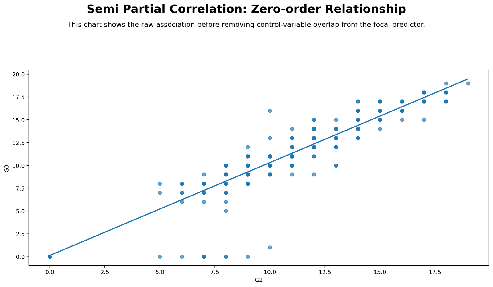
This chart shows the raw association between G2 and G3. The relationship is very strong and positive. Students with higher G2 scores tend to have higher G3 scores. This visual pattern matches the zero-order correlation of r = 0.918548.
The chart is the starting point of the analysis. It tells us that G2 and G3 are strongly related before any controls are considered. However, this chart does not tell us how much of that relationship is unique to G2 after G1, studytime, failures and absences are already included.
That is why the semi partial analysis moves beyond this scatterplot. The zero-order relationship is real and strong, but the research question is about unique contribution, not just raw association.
Python Chart 2: Semi Partial Scatterplot with Residualized Predictor
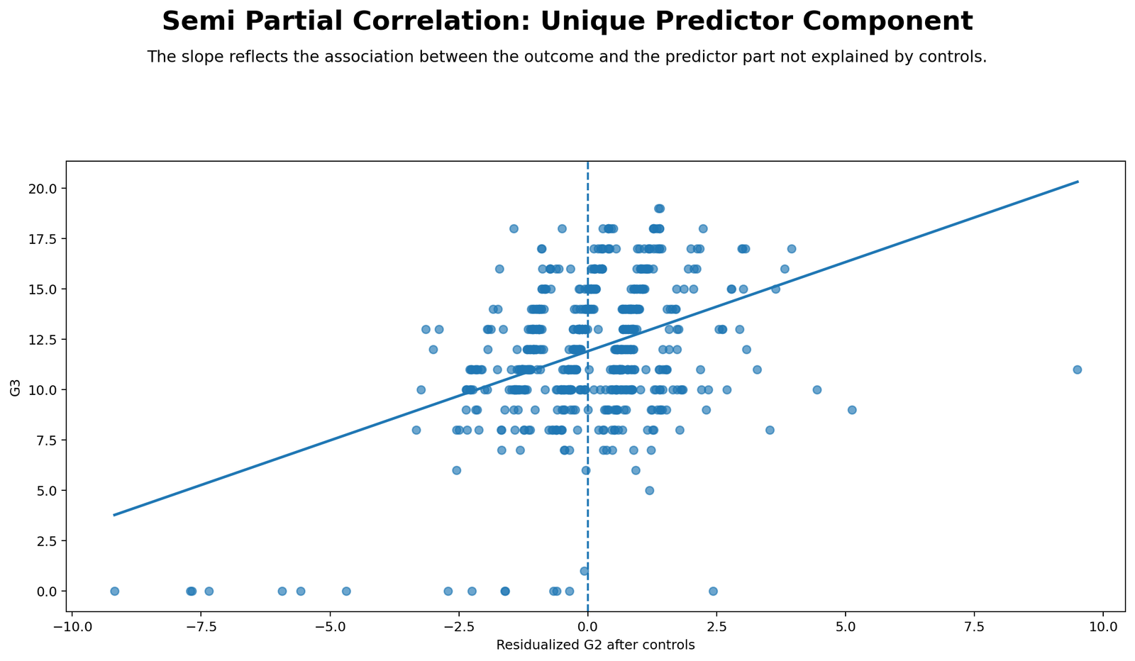
This chart is the core semi partial correlation visual. The x-axis represents the part of G2 that remains after G2 has been predicted from G1, studytime, failures and absences. The y-axis remains the original G3 outcome.
The positive trend shows that the unique part of G2 still relates strongly to G3. The semi partial correlation is sr = 0.397992. This is smaller than the zero-order correlation, but it is still meaningful because it represents unique predictor information after controls.
The chart helps readers understand the difference between ordinary and semi partial correlation. Ordinary correlation uses raw G2. Semi partial correlation uses only the residualized part of G2, then correlates that part with G3.
Python Chart 3: R-Squared Change
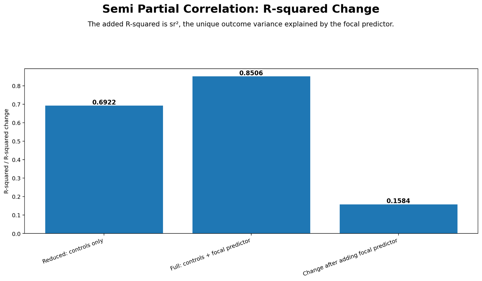
This chart shows the unique variance story directly. The reduced controls-only model has R² = 0.692166. The full model with controls plus G2 has R² = 0.850563. The increase is ΔR² = 0.158397.
This chart is one of the most important visuals because ΔR² equals sr². It shows that adding G2 improves the model by about 15.84% of total G3 variance after the controls have already explained their share.
The correct conclusion is that G2 adds substantial unique explanatory value. The model is not merely statistically significant; it also improves prediction in a practically meaningful way.
Python Chart 4: Correlation Comparison
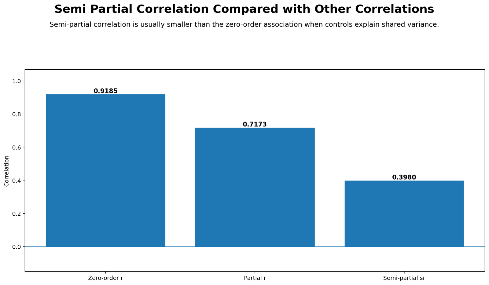
This chart compares three related coefficients: zero-order r, partial r and semi partial sr. The zero-order correlation is 0.918548, the partial correlation is 0.717325, and the semi partial correlation is 0.397992.
The drop from zero-order r to semi partial sr is expected. The semi partial coefficient removes from G2 the part explained by the controls, so it focuses only on the unique part of G2. Even after this removal, the relationship remains positive and meaningful.
This chart is excellent for teaching because it prevents confusion. A reader can see that all three values answer different questions. Zero-order r answers the raw relationship question. Partial r answers the residualized-both-sides question. Semi partial sr answers the unique-predictor-contribution question.
Python Chart 5: Full Model Standardized Coefficients
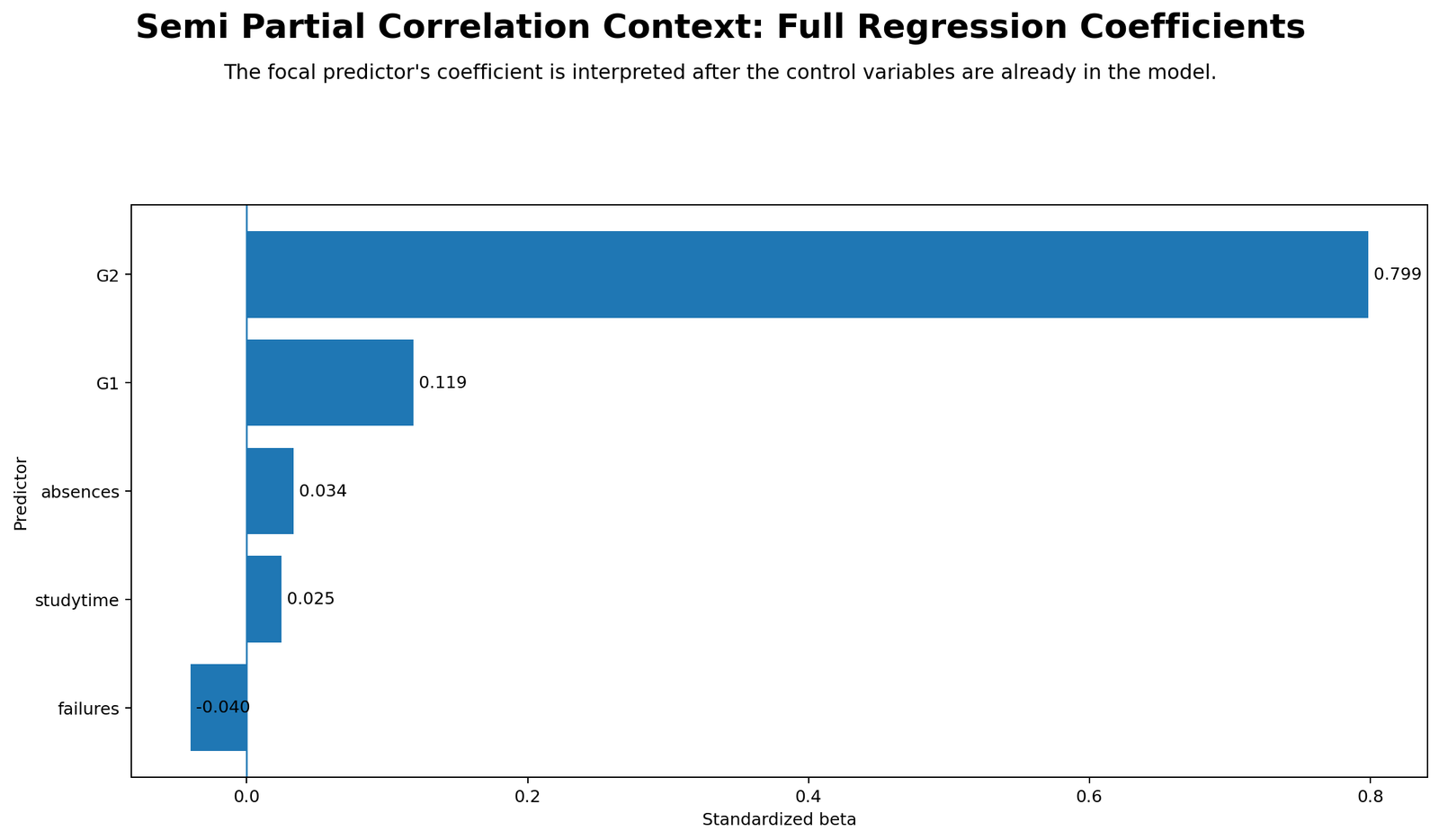
The standardized coefficient chart shows that G2 is the strongest predictor in the full model. The standardized beta for G2 is approximately 0.798796. G1 has a smaller positive beta of about 0.118505, while failures has a small negative beta of about -0.040084.
This chart supports the semi partial result. If G2 has the largest unique standardized effect, it makes sense that adding G2 produces a large R² change. The chart also shows that studytime is not statistically strong in the full model, even though it is conceptually important.
For reporting, this chart should be used to explain predictor importance within the full regression model. The semi partial coefficient gives unique variance; standardized beta gives relative coefficient strength after standardization.
Python Chart 6: Full Model Residuals vs Fitted
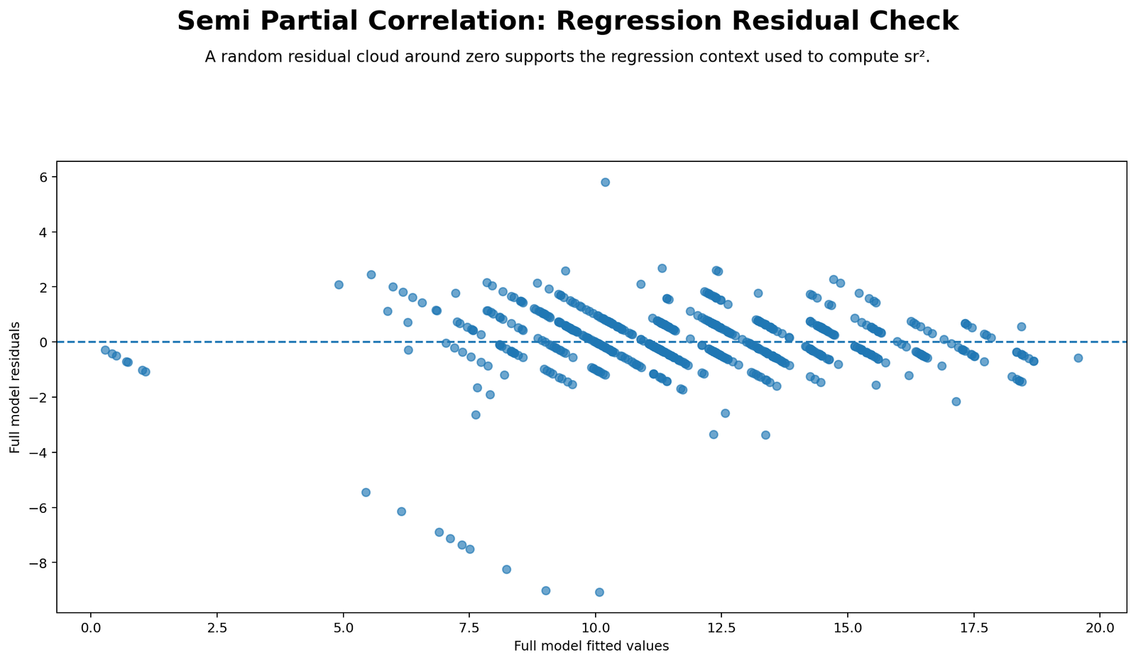
The residuals versus fitted chart checks whether the full regression model behaves reasonably. In a good model, residuals should be scattered around zero without a strong curved pattern. This chart helps evaluate linearity, constant variance and unusual points.
Because semi partial correlation is connected to regression, residual diagnostics are important. A large and significant semi partial correlation can still be affected by nonlinearity, outliers or heteroskedasticity. This chart reminds the reader not to rely only on sr and p-value.
The full model has strong explanatory power, but diagnostics should still be reviewed before final reporting in a research paper or thesis.
R Chart-by-Chart Interpretation
The R assets provide a colorful validation workflow for the same semi partial correlation analysis. The R PDF link returned 404 during verification, but the R chart URLs are included as the assets provided for the post.
R Chart 1: Colorful Zero-Order Scatterplot
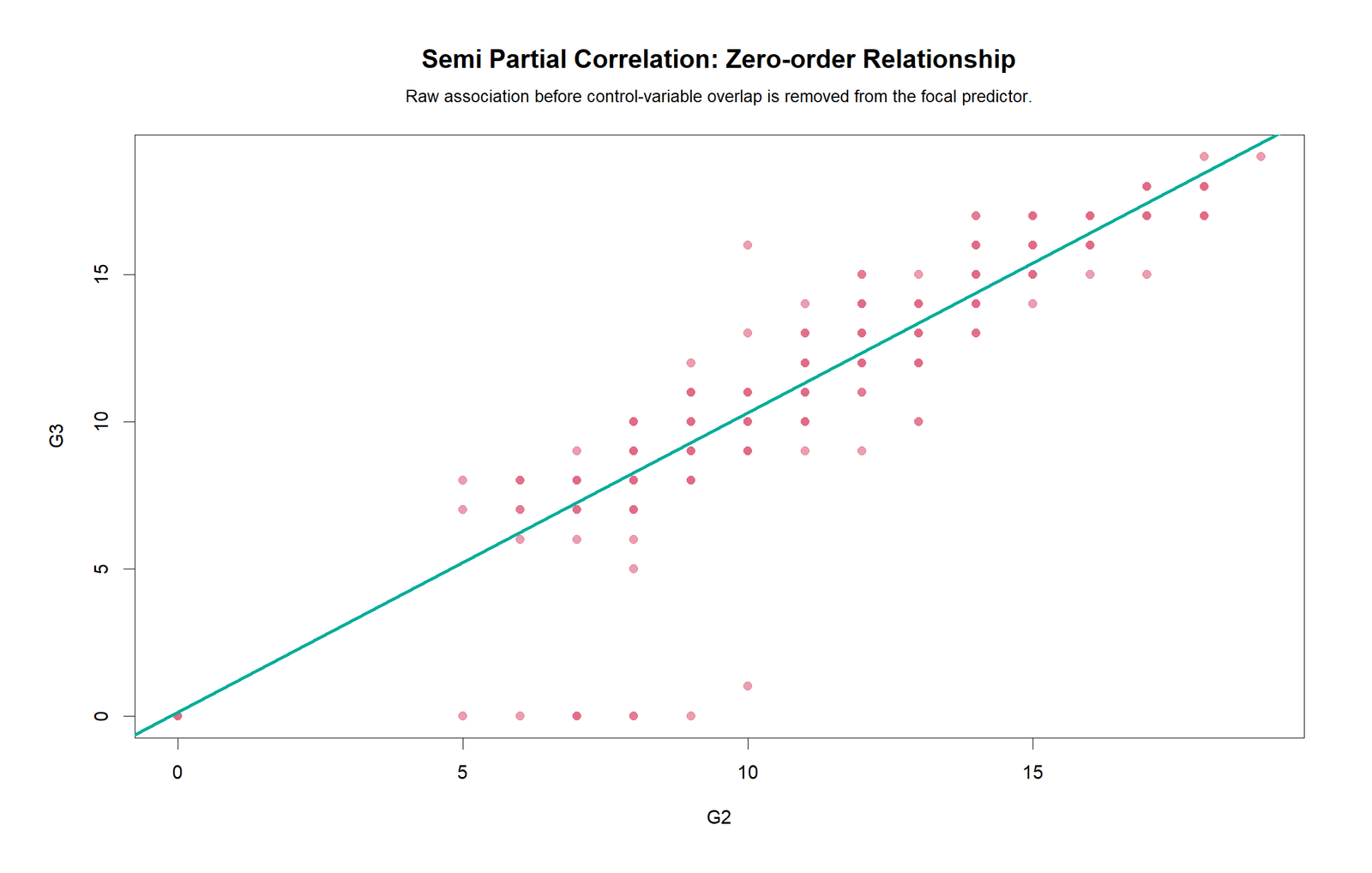
The R zero-order scatterplot repeats the raw G2–G3 relationship. The upward pattern is strong and supports the zero-order r value of 0.918548.
This chart confirms that the strong raw association is visible in both Python and R chart styles. It is a good opening figure for readers because it shows why G2 is a promising predictor before controls are introduced.
R Chart 2: Colorful Semi Partial Scatterplot
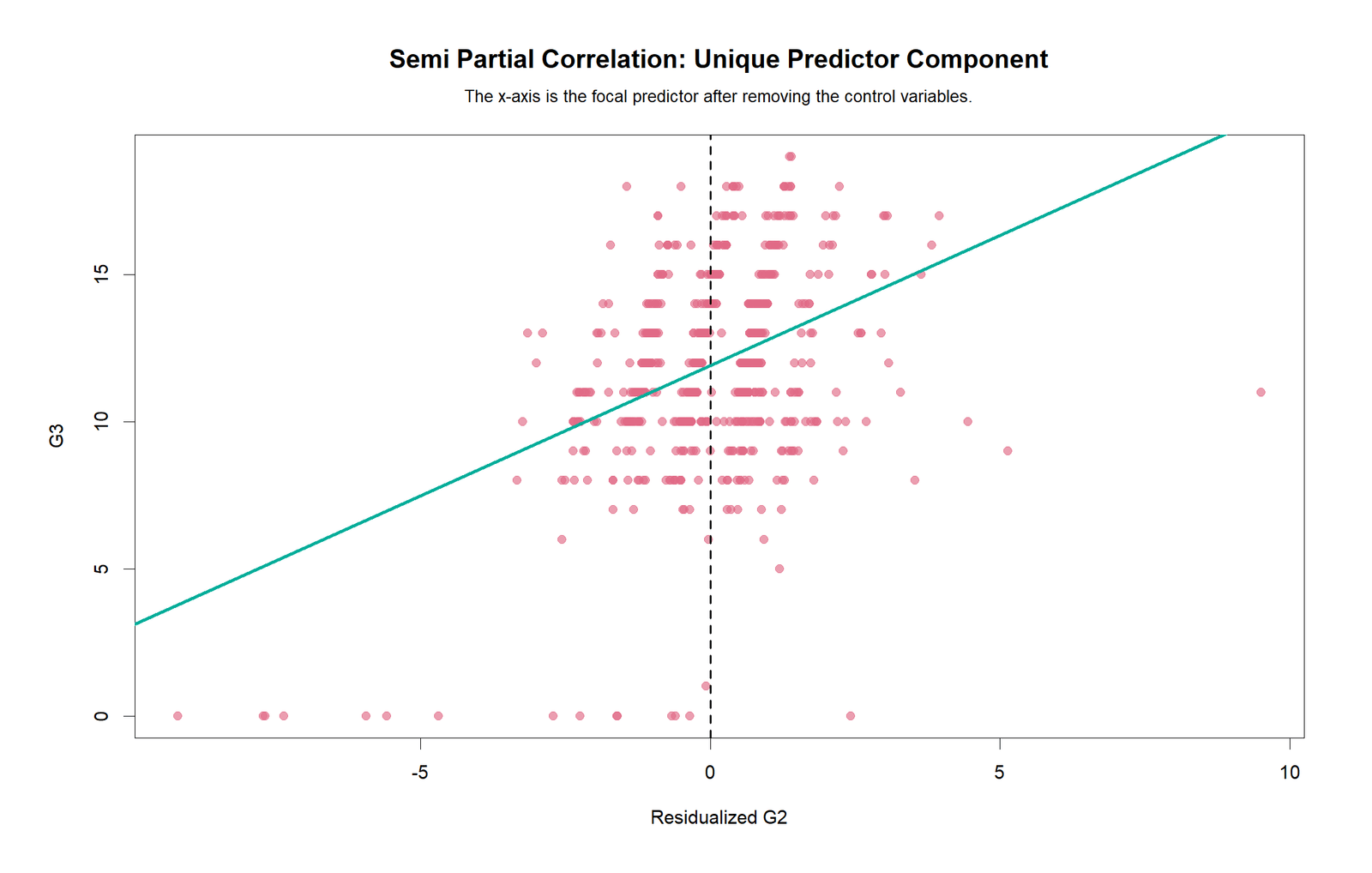
The R residualized-predictor scatterplot shows the semi partial relationship directly. The trend remains positive, indicating that the unique part of G2 is still associated with G3.
This chart gives a visual explanation of sr = 0.397992. The relationship is weaker than the raw zero-order scatterplot but remains meaningful because it represents the unique portion of G2 after control variables have been removed from it.
R Chart 3: Colorful R-Squared Change
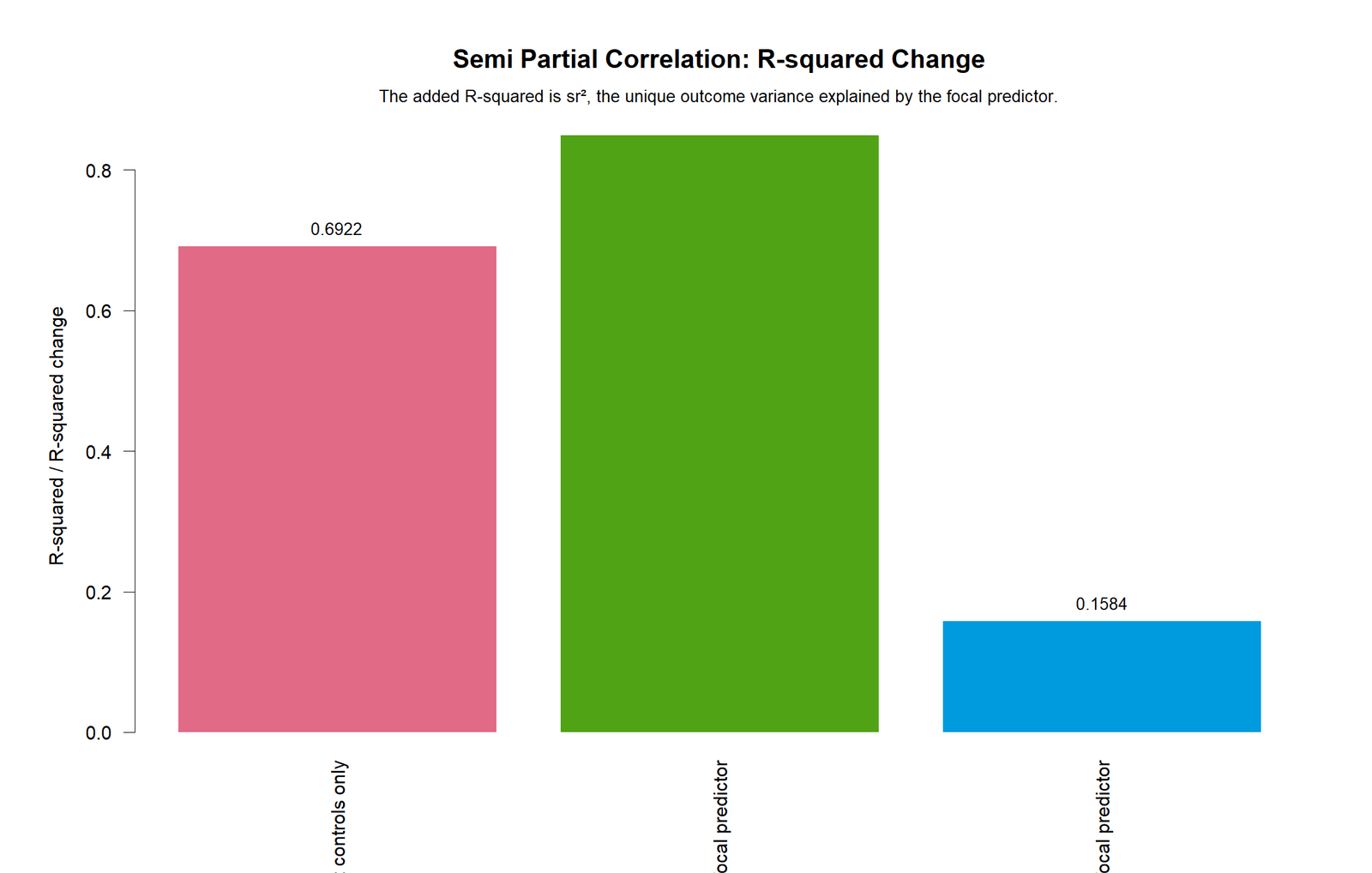
The R R-squared change chart visually confirms the model improvement. The reduced model explains about 69.22% of the variance in G3. The full model explains about 85.06%. The difference is 15.84%.
This is the most direct effect-size interpretation for semi partial correlation. It tells the reader exactly how much additional variance G2 contributes after the controls.
R Chart 4: Colorful Correlation Comparison
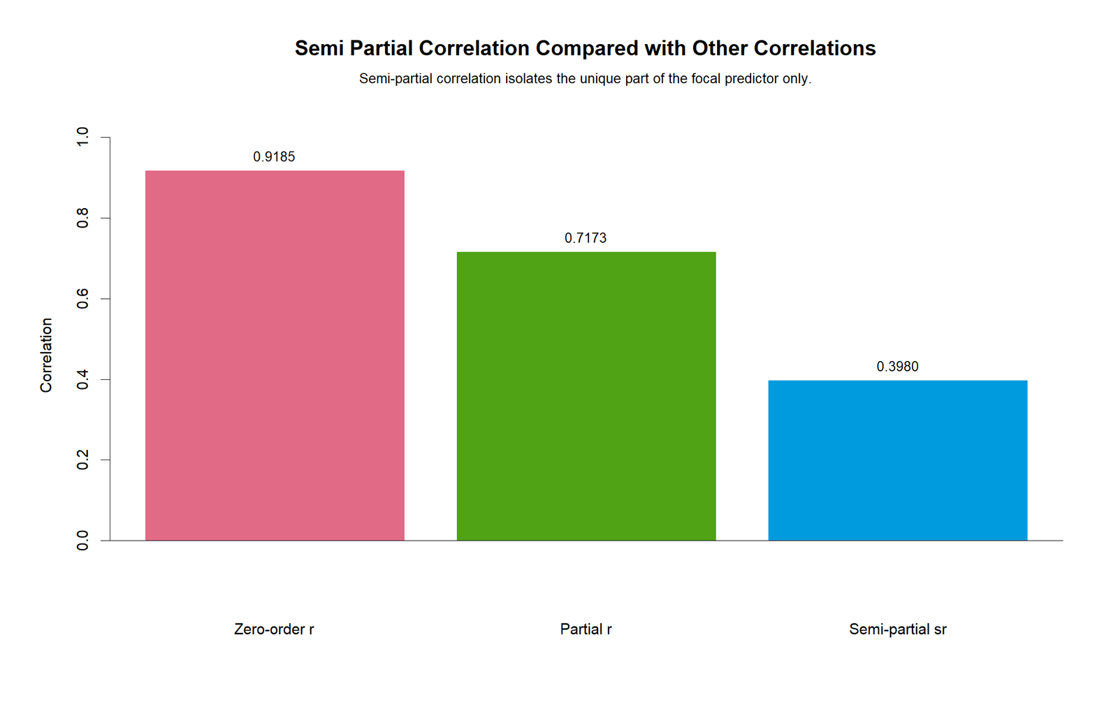
The R correlation comparison chart separates the three coefficient types. It helps readers understand that semi partial sr is not supposed to equal the zero-order correlation or the partial correlation.
The main interpretation is that G2 is highly related to G3 at the raw level, remains strongly related after mutual residualization, and still contributes unique variance when only G2 is residualized.
R Chart 5: Colorful Standardized Coefficients
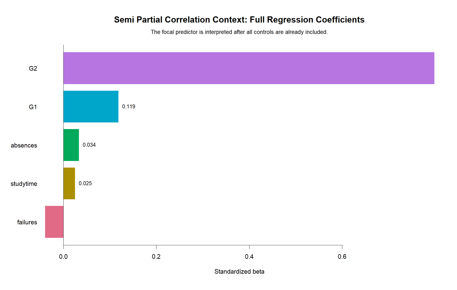
The R standardized coefficient chart confirms that G2 is the dominant predictor. Its standardized beta is far larger than the other predictors in the full model.
This chart should be interpreted with the R² change chart. The coefficient chart shows predictor strength, while the R² change chart shows the unique amount of outcome variance added by G2.
R Chart 6: Colorful Residuals vs Fitted

The R residuals versus fitted plot provides a diagnostic check for the regression model behind the semi partial correlation. It helps detect nonlinearity, unequal residual spread and unusual cases.
The chart belongs in the post because semi partial correlation is not only a correlation idea; it is also a regression-model idea. Good reporting should include both effect size and model diagnostics.
SPSS Output and Workflow Interpretation
The SPSS output link is included in the resources section as provided. During verification, the SPSS PDF link returned a 404 response, so the numerical SPSS interpretation below is based on the verified Excel workbook and Python report values, not on additional unread SPSS-only output.
In SPSS, semi partial correlation is usually read from the Part column in the regression coefficients table. The Part value for the focal predictor is the semi partial correlation. Squaring the Part value gives the unique variance explained by that predictor.
| SPSS Step | Action | Purpose |
|---|---|---|
| 1 | Analyze → Regression → Linear | Open the linear regression dialog. |
| 2 | Put G3 in Dependent | G3 is the outcome variable. |
| 3 | Put G1, studytime, failures and absences in Block 1 | These are the control variables. |
| 4 | Put G2 in Block 2 | G2 is added last to test unique contribution. |
| 5 | Request R squared change statistics | Shows ΔR² and F change. |
| 6 | Request Part and Partial correlations in coefficients | Part is the semi partial correlation. |
| 7 | Interpret the G2 Part column | Expected semi partial sr is about 0.398. |
In SPSS-style reporting, the result should be written as a hierarchical regression or part-correlation result: adding G2 after G1, studytime, failures and absences significantly increased R² by 0.158, with sr = .398, p < .001.
Excel Worked File Explanation
The Excel workbook is a fully worked semi partial correlation file. It includes the dataset, inputs, working data, regression formulas, semi partial result table, verified results table, chart data and interpretation guidance.
Download the Semi Partial Correlation Fully Worked Excel File
Download the Semi Partial Correlation Keyword Workbook
| Excel Sheet | Purpose | What It Teaches |
|---|---|---|
| README | Explains workbook purpose. | Defines semi partial correlation and the main formula. |
| Dataset | Stores the raw data. | Keeps the workbook self-contained. |
| Inputs | Defines outcome, focal predictor, controls and alpha. | Shows the model setup clearly. |
| Working Data | Stores selected variables, predictions and residuals. | Shows how G2 is residualized on controls. |
| Regression Formulas | Shows coefficient formulas and model statistics. | Explains reduced model, full model and focal residual model. |
| Semi Partial Result | Formula-driven result table. | Reports sr, sr², R² change, F change and p-value. |
| Verified Results | Static verified values. | Provides audit-ready output values. |
| Charts Data | Chart-ready values. | Feeds correlation comparison and R² change charts. |
| Interpretation | Plain-language result guide. | Provides a report sentence and interpretation summary. |
Excel Formula Logic
The workbook calculates semi partial correlation in two equivalent ways. First, it correlates G3 with residualized G2. Second, it calculates R² change and takes the signed square root.
| Step | Excel Formula / Method | Purpose |
|---|---|---|
| Predict G2 from controls | LINEST or regression formulas | Find the part of G2 explained by G1, studytime, failures and absences. |
| Calculate residualized G2 | Actual G2 − predicted G2 | Find the unique part of G2. |
| Calculate semi partial sr | =CORREL(G3_range,residualized_G2_range) | Correlation between outcome and unique part of G2. |
| Reduced R² | =RSQ(predicted_G3_controls_only,G3_range) | Controls-only model variance explained. |
| Full R² | =RSQ(predicted_G3_full_model,G3_range) | Controls plus G2 model variance explained. |
| R² change | =Full_R2-Reduced_R2 | Unique variance explained by G2. |
| Check sr² | =sr^2 | Should equal R² change. |
| F change | =(R2_change/df1)/((1-Full_R2)/df2) | Test whether adding G2 improves the model. |
| p-value | =F.DIST.RT(F_change,df1,df2) | Significance of unique contribution. |
The Excel interpretation sheet summarizes the result in one sentence: G2 made a significant unique contribution to G3 after controlling G1, studytime, failures and absences, sr = 0.398, sr² = 0.158, p < .001.
Python, R, SPSS and Excel Workflows
The same semi partial correlation result can be reproduced in Python, R, SPSS and Excel. The important requirement is that the same outcome, focal predictor, controls and missing-value rule are used.
| Software | Main Workflow | Best Use |
|---|---|---|
| Python | Use regression to residualize G2 on controls, correlate residualized G2 with G3, compare reduced and full R², and export charts. | Automated chart generation, reproducible reporting and PDF summaries. |
| R | Use lm() models for reduced and full regression, residualize the focal predictor, calculate sr and plot colorful validation charts. | Statistical validation and publication-style charts. |
| SPSS | Run hierarchical regression and read the Part column for G2 in the coefficients table. | Formal output table for thesis, assignments and research reports. |
| Excel | Use regression formulas, residual calculations, CORREL, RSQ, F.DIST.RT and dashboard formulas. | Step-by-step teaching and transparent formula verification. |
Code Blocks and Excel Formulas
Python Code for Semi Partial Correlation
import pandas as pd
import numpy as np
from scipy import stats
from sklearn.linear_model import LinearRegression

df = pd.read_csv("dataset.csv")

outcome = "G3"
focal = "G2"
controls = ["G1", "studytime", "failures", "absences"]

work = df[[outcome, focal] + controls].dropna().copy()
for col in [outcome, focal] + controls:
    work[col] = pd.to_numeric(work[col], errors="coerce")
work = work.dropna()

Y = work[outcome].to_numpy()
X_focal = work[focal].to_numpy()
X_controls = work[controls].to_numpy()

# Zero-order correlation
zero_r, zero_p = stats.pearsonr(X_focal, Y)

# Residualize focal predictor on controls
model_focal = LinearRegression().fit(X_controls, X_focal)
focal_pred = model_focal.predict(X_controls)
focal_resid = X_focal - focal_pred

# Semi-partial correlation: outcome with residualized focal predictor
sr, sr_p_simple = stats.pearsonr(Y, focal_resid)
sr2 = sr ** 2

# Reduced model: controls only
reduced_model = LinearRegression().fit(X_controls, Y)
yhat_reduced = reduced_model.predict(X_controls)
reduced_r2 = reduced_model.score(X_controls, Y)

# Full model: controls + focal
X_full = work[controls + [focal]].to_numpy()
full_model = LinearRegression().fit(X_full, Y)
yhat_full = full_model.predict(X_full)
full_r2 = full_model.score(X_full, Y)

r2_change = full_r2 - reduced_r2

n = len(work)
p_full = len(controls) + 1
df1 = 1
df2 = n - p_full - 1
f_change = (r2_change / df1) / ((1 - full_r2) / df2)
p_change = stats.f.sf(f_change, df1, df2)

print("N:", n)
print("Zero-order r:", zero_r)
print("Semi-partial sr:", sr)
print("sr squared:", sr2)
print("Reduced R2:", reduced_r2)
print("Full R2:", full_r2)
print("R2 change:", r2_change)
print("F change:", f_change)
print("df1:", df1, "df2:", df2)
print("p-value:", p_change)
R Code for Semi Partial Correlation
df <- read.csv("dataset.csv", stringsAsFactors = FALSE)

vars <- c("G3", "G2", "G1", "studytime", "failures", "absences")
work <- na.omit(df[vars])
work[] <- lapply(work, as.numeric)

# Zero-order correlation
zero_test <- cor.test(work$G2, work$G3, method = "pearson")

# Residualize G2 on controls
focal_resid <- resid(lm(G2 ~ G1 + studytime + failures + absences, data = work))

# Semi-partial correlation
sr_test <- cor.test(work$G3, focal_resid, method = "pearson")
sr <- unname(sr_test$estimate)
sr2 <- sr^2

# Reduced and full models
reduced <- lm(G3 ~ G1 + studytime + failures + absences, data = work)
full <- lm(G3 ~ G1 + studytime + failures + absences + G2, data = work)

reduced_r2 <- summary(reduced)$r.squared
full_r2 <- summary(full)$r.squared
r2_change <- full_r2 - reduced_r2

anova_change <- anova(reduced, full)

cat("Zero-order r:", unname(zero_test$estimate), "\n")
cat("Semi-partial sr:", sr, "\n")
cat("sr squared:", sr2, "\n")
cat("Reduced R2:", reduced_r2, "\n")
cat("Full R2:", full_r2, "\n")
cat("R2 change:", r2_change, "\n")
print(anova_change)
summary(full)
SPSS Syntax for Semi Partial Correlation
* Semi Partial Correlation / Part Correlation in SPSS.
* Outcome: G3.
* Focal predictor: G2.
* Controls: G1 studytime failures absences.

OUTPUT CLOSE ALL.
OUTPUT NEW NAME=Semi_Partial_Correlation_Output.

DESCRIPTIVES VARIABLES=G3 G2 G1 studytime failures absences
  /STATISTICS=MEAN STDDEV MIN MAX.

CORRELATIONS
  /VARIABLES=G3 G2 G1 studytime failures absences
  /PRINT=TWOTAIL
  /MISSING=PAIRWISE.

REGRESSION
  /DEPENDENT G3
  /METHOD=ENTER G1 studytime failures absences
  /METHOD=ENTER G2
  /STATISTICS COEFF OUTS R ANOVA CHANGE ZPP CI(95)
  /DEPENDENT G3
  /SAVE PRED RESID.

* In the Coefficients table, read the Part column for G2.
* Part for G2 is the semi-partial correlation.
* Part squared is the unique variance added by G2.

OUTPUT EXPORT
  /CONTENTS EXPORT=VISIBLE
  /PDF DOCUMENTFILE='Semi-Partial-Correlation-SPSS-Output.pdf'.
Excel Formula Patterns
Outcome:
G3_range

Focal predictor:
G2_range

Controls:
G1_range, studytime_range, failures_range, absences_range

Semi-partial sr:
=CORREL(G3_range, residualized_G2_range)

Residualized G2:
=G2_actual - G2_predicted_from_controls

Reduced R squared:
=RSQ(predicted_G3_controls_only, G3_range)

Full R squared:
=RSQ(predicted_G3_full_model, G3_range)

R squared change:
=Full_R2 - Reduced_R2

sr squared:
=sr^2

Check:
sr^2 should equal R_squared_change

df2:
=N - number_of_full_model_predictors - 1

F change:
=(R2_change/1)/((1-Full_R2)/df2)

p-value:
=F.DIST.RT(F_change,1,df2)

Decision:
=IF(p_value<0.05,"Significant unique contribution","Not significant")
Assumptions and Diagnostics
Semi partial correlation is based on regression, so its assumptions overlap with multiple linear regression assumptions. The coefficient should be interpreted after reviewing model fit, residual behavior and predictor overlap.
| Assumption / Diagnostic | Meaning | How to Check | Why It Matters Here |
|---|---|---|---|
| Numeric variables | Outcome and predictors should be numeric or properly coded. | Review variable types and descriptive statistics. | G3, G2, G1, studytime, failures and absences are numeric-coded variables. |
| Linearity | Relationships should be approximately linear. | Use scatterplots and residual plots. | Zero-order and residualized-predictor scatterplots help check this. |
| Independent observations | Rows should not be repeated or dependent observations. | Review study design. | Each row should represent a separate student observation. |
| No extreme influential outliers | Outliers can affect regression coefficients and sr. | Use residual diagnostics, leverage and Cook's distance. | Grade data may include low-score points that should be reviewed. |
| Homoscedasticity | Residual spread should be reasonably stable across fitted values. | Use residuals versus fitted chart. | The Python and R residual charts support this diagnostic step. |
| No problematic multicollinearity | Predictors should not be too redundant for stable interpretation. | Check VIF and correlations among predictors. | G1 and G2 are strongly related, so interpretation should emphasize unique contribution. |
| Theoretical control selection | Controls should be chosen for a reason. | Justify controls in the methods section. | G1, studytime, failures and absences are meaningful controls for final grade. |
Because G1 and G2 are both grade variables, multicollinearity and shared academic-performance information should be discussed carefully. The result is still strong, but the report should make clear that G2 is being evaluated after G1 and other controls are already in the model.
How to Report Semi Partial Correlation
A complete report should include the outcome, focal predictor, controls, sr, sr² or ΔR², model R² values, F change, degrees of freedom, p-value and interpretation.
APA-style report: A hierarchical regression was used to evaluate the unique contribution of G2 to G3 after controlling for G1, studytime, failures and absences. The controls-only model explained 69.22% of the variance in G3, R² = .692. Adding G2 increased the explained variance to 85.06%, R² = .851, ΔR² = .158. The semi-partial correlation for G2 was significant, sr = .398, sr² = .158, F change(1, 643) = 681.56, p < .001. This indicates that G2 made a substantial unique contribution to G3 after the controls were included.
Short report: G2 made a significant unique contribution to G3 after controlling for G1, studytime, failures and absences, sr = .398, sr² = .158, p < .001.
Interpretive report: The zero-order G2–G3 correlation was very strong, r = .919. After isolating the unique portion of G2 not explained by the controls, G2 still explained an additional 15.84% of the variance in G3. This makes G2 the dominant unique predictor in the full model.
Common Mistakes in Semi Partial Correlation Interpretation
| Mistake | Why It Is a Problem | Better Practice |
|---|---|---|
| Confusing semi partial and partial correlation | They residualize different variables and answer different questions. | Use semi partial for unique variance added by the focal predictor. |
| Reporting sr without sr² | sr² is the direct unique variance interpretation. | Report both sr and sr² or ΔR². |
| Ignoring model order | sr depends on what controls are entered before the focal predictor. | Clearly state the controls and that G2 was added last. |
| Calling semi partial correlation a raw correlation | sr uses residualized focal predictor, not raw X. | Say “G3 correlated with residualized G2.” |
| Ignoring multicollinearity | Strong predictor overlap can affect coefficient interpretation. | Check VIF and predictor correlations. |
| Reporting only p-value | p-value does not show unique effect size. | Report sr, sr², R² change and p-value. |
| Claiming causation | Semi partial correlation is still observational unless design supports causality. | Use “unique association” or “unique contribution.” |
| Skipping residual diagnostics | Regression assumptions matter for interpretation. | Use residuals vs fitted and outlier diagnostics. |
Downloads and Resources
Download Excel Worked FileFully worked Excel file with formulas, residualized predictor, R² change and verified results.
Download Keyword WorkbookBroad-match keyword file for Semi Partial Correlation SEO planning.
Open Python R² Change ChartChart showing reduced model R², full model R² and unique variance added by G2.
External References
For additional learning, review regression textbooks and software documentation on part correlation, partial correlation, hierarchical regression, R-squared change, standardized coefficients, residual diagnostics and model comparison.
FAQs About Semi Partial Correlation
What is Semi Partial Correlation?
Semi partial correlation is the correlation between an outcome and the unique part of a predictor after that predictor has been residualized on control variables.
What is the main result in this guide?
G2 made a significant unique contribution to G3 after controlling G1, studytime, failures and absences, sr = 0.397992, sr² = 0.158397, p < .001.
What does sr squared mean?
sr² is the unique proportion of outcome variance explained by the focal predictor. Here, sr² = 0.158397, meaning G2 adds about 15.84% unique explained variance in G3 after controls.
Is semi partial correlation the same as partial correlation?
No. Partial correlation residualizes both the outcome and predictor. Semi partial correlation residualizes only the focal predictor and correlates that residualized predictor with the original outcome.
Why is semi partial correlation useful in regression?
It shows the unique contribution of one predictor after other predictors are already in the model. Its squared value equals the R² change when the predictor is added last.
How do I read semi partial correlation in SPSS?
Run linear regression and request Part and Partial correlations in the coefficients table. The Part column for the focal predictor is the semi partial correlation.
Can Excel calculate semi partial correlation?
Yes. Excel can calculate it by residualizing the focal predictor using regression formulas, then using CORREL between the outcome and the residualized predictor. It can also calculate sr² as the R² change between reduced and full models.
What is the APA-style sentence for this result?
A semi partial correlation showed that G2 made a significant unique contribution to G3 after controlling for G1, studytime, failures and absences, sr = .398, sr² = .158, F change(1, 643) = 681.56, p < .001.
Does semi partial correlation prove causation?
No. Semi partial correlation measures unique statistical association. It does not prove causation unless the research design supports causal inference.
Why is the zero-order correlation larger than the semi partial correlation?
The zero-order correlation uses raw G2 and raw G3. Semi partial correlation uses only the part of G2 that is not explained by the controls, so it is usually smaller and more specific.

