
Post Hoc ANOVA, Tukey-Kramer Comparisons and Familywise Error Control
Tukey HSD Test: Formula, Interpretation, SPSS, Python, R and Excel Guide
Tukey HSD Test, also called Tukey’s Honestly Significant Difference test, is a post hoc procedure used after a statistically significant one-way ANOVA to compare all possible pairs of group means while controlling the familywise error rate. This guide explains the Tukey HSD Test with SPSS output, Python charts, R validation charts, Tukey-Kramer unequal sample size logic, simultaneous confidence intervals, adjusted p-values, APA reporting, Excel workflow and downloadable resources.
Quick Answer: Tukey HSD Test Result
The worked example compares G3 final grade across four studytime groups. The one-way ANOVA was statistically significant, F(3, 645) = 15.876, p < .001, so post hoc pairwise comparisons were justified. The median-centered Levene / Brown-Forsythe variance context was not significant, p = .380, so the equal-variance context looked reasonable for Tukey HSD.
The Tukey HSD Test showed that 4 of the 6 pairwise comparisons were significant at alpha .05. Studytime group 1, students studying less than 2 hours, had the lowest mean G3 score, M = 10.844. Studytime group 3, students studying 5 to 10 hours, had the highest mean, M = 13.227, followed closely by studytime group 4, students studying more than 10 hours, M = 13.057. The strongest difference was between studytime group 1 and group 3, mean difference = 2.382, q = 8.796, adjusted p < .001.
Final interpretation: The Tukey HSD post hoc test indicates that final grades differ mainly between the lowest studytime group and the higher studytime groups. Students in studytime group 1 scored significantly lower than groups 2, 3 and 4. Group 2 was also significantly lower than group 3. The differences between groups 2 and 4 and between groups 3 and 4 were not statistically significant.
Important reporting point: Tukey HSD should normally be interpreted after the omnibus ANOVA shows evidence of mean differences. It is designed for all pairwise comparisons and controls the familywise error rate better than running many unadjusted t tests.
Table of Contents
- What Is the Tukey HSD Test?
- When Should You Use Tukey HSD?
- Tukey HSD Formula and Tukey-Kramer Formula
- Hypotheses and Decision Rule
- Dataset and Variables Used
- ANOVA and Assumption Context
- Tukey HSD Pairwise Results
- SPSS Output Interpretation
- Python Chart-by-Chart Interpretation
- R Chart-by-Chart Validation
- SPSS, R, Python and Excel Workflows
- Code Blocks for Tukey HSD Test
- APA Reporting Wording
- Common Mistakes
- Downloads and Resources
- Related Guides
- External References
- FAQs
What Is the Tukey HSD Test?
The Tukey HSD Test is a multiple-comparison procedure used after ANOVA when a researcher wants to know exactly which group means differ. ANOVA tells whether at least one group mean is different, but it does not identify the specific pairs. Tukey HSD fills that gap by comparing every pair of group means with one familywise error-controlled procedure.
The name HSD means Honestly Significant Difference. In a balanced design, Tukey HSD compares each absolute mean difference with a single critical difference. In an unequal sample size design, the Tukey-Kramer version adjusts the standard error for each pair using the two sample sizes in that pair. Because the studytime groups in this example have unequal sample sizes, the Tukey-Kramer logic is the correct interpretation.
Simple definition: Tukey HSD asks: after ANOVA, which specific group means are far enough apart to be called significantly different while still protecting the overall family of pairwise tests?
The Tukey HSD Test is closely connected to one-way ANOVA, ANOVA assumptions, p-values, confidence intervals, and effect size. It should not be treated as a replacement for ANOVA. It is a follow-up procedure that gives pairwise detail after the omnibus test.
When Should You Use Tukey HSD?
Use the Tukey HSD Test when the dependent variable is numeric, the independent variable has three or more groups, and the main research question involves all pairwise comparisons among group means. It is especially useful after a one-way ANOVA because it keeps the familywise Type I error rate under control when multiple pairs are tested.
| Condition | Tukey HSD Requirement | Worked Example |
|---|---|---|
| Dependent variable | Continuous or approximately numeric outcome | G3 final grade |
| Factor variable | Three or more independent groups | studytime with 4 groups |
| Omnibus test | ANOVA should show meaningful overall differences | F(3, 645) = 15.876, p < .001 |
| Variance context | Equal variances should look reasonable | Median-centered Levene / Brown-Forsythe p = .380 |
| Comparison goal | All pairwise group comparisons | 6 pairwise comparisons among 4 studytime groups |
If equal variances are clearly violated, Tukey HSD may not be the best post hoc test. In that situation, compare with unequal-variance procedures such as Games-Howell or Tamhane’s T2. For assumption checking, see Levene’s test, Brown-Forsythe test, balanced ANOVA, and ANOVA in SPSS.
Tukey HSD Formula and Tukey-Kramer Formula
For equal group sizes, the Tukey HSD critical difference is calculated using the Studentized range critical value, the ANOVA mean square error and the common group sample size.
When sample sizes are unequal, the Tukey-Kramer denominator changes by pair. This is the version used in the Python and R reports for this example.
| Symbol | Meaning | Value in This Example |
|---|---|---|
| qcritical | Studentized range critical value | 3.642648 |
| k | Number of groups | 4 |
| df | ANOVA within/error degrees of freedom | 645 |
| MSE | ANOVA mean square within/error | 9.764634 |
| ni, nj | Sample sizes for the pair | Different for each studytime pair |
Hypotheses and Decision Rule for Tukey HSD
The Tukey HSD Test evaluates each pair of group means. For any pair, the null hypothesis says the two population means are equal. The alternative hypothesis says the two population means are different.
| Comparison Level | Hypothesis | Meaning |
|---|---|---|
| Pairwise null hypothesis | H0: μi = μj | The two studytime groups have equal mean G3 scores. |
| Pairwise alternative hypothesis | H1: μi ≠ μj | The two studytime groups have different mean G3 scores. |
| Decision by adjusted p-value | Reject H0 if adjusted p < .05 | The pair is statistically significant after familywise adjustment. |
| Decision by confidence interval | Reject H0 if simultaneous CI excludes 0 | The mean difference is reliably different from zero. |
| Decision by q statistic | Reject H0 if q > qcritical | The observed mean gap exceeds the Tukey critical rule. |
Dataset and Variables Used
The worked example uses the student performance dataset structure commonly used in Salar Cafe statistical guides. The dependent variable is G3, the final grade. The grouping variable is studytime, which has four ordered categories. This makes it a suitable example for one-way ANOVA followed by Tukey HSD Test post hoc comparisons.
| Variable | Role | Interpretation in This Guide |
|---|---|---|
| G3 | Dependent variable | Final grade / numeric outcome being compared across groups. |
| studytime | Factor variable | Four study-time groups used for ANOVA and Tukey HSD comparisons. |
| Group 1 | <2 hours | Lowest mean G3 score in this analysis. |
| Group 2 | 2 to 5 hours | Intermediate mean G3 score. |
| Group 3 | 5 to 10 hours | Highest mean G3 score. |
| Group 4 | >10 hours | High mean G3 score but small sample size compared with groups 1 and 2. |
ANOVA and Assumption Context Before Tukey HSD
The ANOVA result is the first decision point. The between-group sum of squares was 465.078, the within-group sum of squares was 6298.189, and the within-group mean square error was 9.765. The omnibus ANOVA result was F(3, 645) = 15.876, p < .001, which supports moving to post hoc pairwise interpretation.
The variance context also supports Tukey HSD interpretation. The median-centered Levene / Brown-Forsythe context was F = 1.026, p = .380. Because this p-value is greater than .05, the equal-variance assumption does not show a serious warning in this example. The robust Welch and Brown-Forsythe tests were also significant, which confirms that the group mean pattern is not limited to the ordinary ANOVA table.
| Output Item | Value | Interpretation |
|---|---|---|
| Total N | 649 | All valid cases used in the ANOVA and post hoc workflow. |
| Number of groups | 4 | Six pairwise comparisons are possible. |
| Grand mean | 11.906 | Overall mean final grade across all studytime groups. |
| ANOVA | F(3, 645) = 15.876, p < .001 | At least one studytime group mean differs from another. |
| Eta squared | .0688 | About 6.9% of G3 variance is associated with studytime group differences. |
| Omega squared | .0643 | A slightly corrected estimate of the practical ANOVA effect. |
| Median-centered Levene / Brown-Forsythe context | F = 1.026, p = .380 | Equal-variance context looks acceptable for Tukey HSD. |
Tukey HSD Pairwise Results
The table below summarizes the Tukey-Kramer pairwise comparisons. A comparison is significant when the adjusted p-value is below .05, the simultaneous confidence interval does not include zero, and the q statistic is above the Tukey critical q value of 3.642648.
| Pair | Mean Difference | q Statistic | Simultaneous 95% CI | Adjusted p | Decision |
|---|---|---|---|---|---|
| Studytime 1 vs 2 | 1.247 | 6.314 | 0.528 to 1.967 | < .001 | Significant |
| Studytime 1 vs 4 | 2.213 | 5.489 | 0.744 to 3.681 | .001 | Significant |
| Studytime 1 vs 3 | 2.382 | 8.796 | 1.396 to 3.369 | < .001 | Significant |
| Studytime 2 vs 4 | 0.965 | 2.448 | -0.471 to 2.402 | .308 | Not significant |
| Studytime 2 vs 3 | 1.135 | 4.407 | 0.197 to 2.073 | .010 | Significant |
| Studytime 4 vs 3 | 0.170 | 0.389 | -1.417 to 1.757 | .993 | Not significant |
Pairwise conclusion: The main finding is that the lowest studytime group is significantly lower than the higher studytime groups. Group 3 is also significantly higher than group 2. However, the differences between groups 2 and 4 and between groups 3 and 4 are not statistically significant.
SPSS Output Interpretation for Tukey HSD Test
The SPSS output confirms the complete workflow: descriptive statistics by studytime group, homogeneity of variances, one-way ANOVA, robust tests, Tukey HSD multiple comparisons and homogeneous subsets. The SPSS one-way ANOVA command used G3 as the dependent variable and studytime as the grouping factor, with Tukey post hoc comparisons at alpha .05.
SPSS Descriptive Statistics
| Studytime Group | N | Mean G3 | Std. Deviation | Std. Error | 95% CI for Mean | Minimum-Maximum |
|---|---|---|---|---|---|---|
| 1: <2 hours | 212 | 10.8443 | 3.2186 | .2211 | 10.4086 to 11.2801 | 0 to 18 |
| 2: 2 to 5 hours | 305 | 12.0918 | 3.2431 | .1857 | 11.7264 to 12.4572 | 0 to 19 |
| 3: 5 to 10 hours | 97 | 13.2268 | 2.5021 | .2541 | 12.7225 to 13.7311 | 8 to 18 |
| 4: >10 hours | 35 | 13.0571 | 3.0384 | .5136 | 12.0134 to 14.1009 | 6 to 19 |
| Total | 649 | 11.9060 | 3.2307 | .1268 | 11.6570 to 12.1550 | 0 to 19 |
SPSS ANOVA and Homogeneity Results
The SPSS homogeneity output showed non-significant Levene-style tests. Based on the mean, Levene’s statistic was .985, p = .400. Based on the median, the statistic was 1.026, p = .380. These values do not indicate a serious variance problem for Tukey HSD interpretation.
The ANOVA table showed SSbetween = 465.078, SSwithin = 6298.189, dfbetween = 3, dfwithin = 645, MSbetween = 155.026, MSwithin = 9.765, and F = 15.876, p < .001. This confirms that the group means are not all equal.
SPSS Tukey HSD Multiple Comparisons
The SPSS multiple-comparisons table marks significant mean differences with an asterisk. Studytime 1 differed significantly from studytime 2, 3 and 4. Studytime 2 differed significantly from studytime 3. The comparisons between studytime 2 and 4 and between studytime 3 and 4 were not significant. This matches the Python and R post hoc summaries.
SPSS interpretation summary: G3 differs by studytime group. The lowest studytime group has the lowest final grade mean, and Tukey HSD shows that several higher studytime groups are significantly above it. Because not all higher studytime groups differ from one another, the interpretation should emphasize the pattern rather than claiming that every increase in studytime creates a statistically separate mean.
Python Chart-by-Chart Interpretation
The Python charts show the Tukey HSD result from several angles: simultaneous confidence intervals, group means and letters, q statistics, mean differences versus HSD thresholds, pairwise decision matrix, adjusted p-values, ANOVA variance decomposition and distribution context.
Python Chart 1: Tukey HSD Simultaneous Confidence Interval Forest
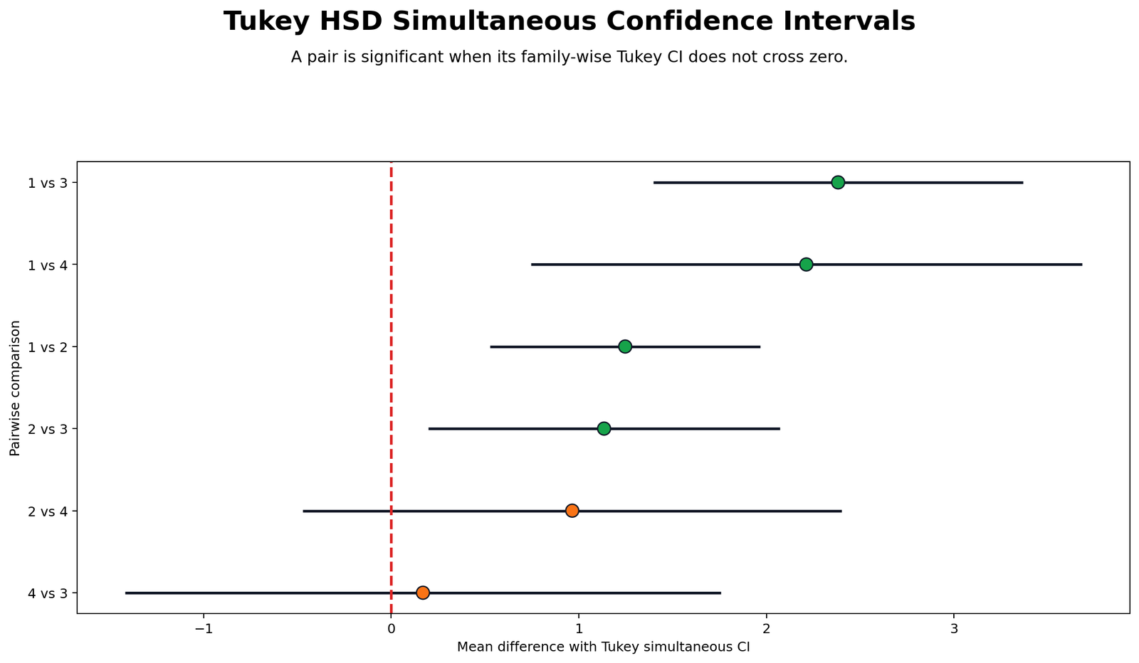
This forest chart shows each pairwise mean difference with its simultaneous confidence interval. A Tukey comparison is significant when the interval stays completely away from zero. The intervals for studytime 1 versus 2, studytime 1 versus 3, studytime 1 versus 4, and studytime 2 versus 3 exclude zero, so they are significant at alpha .05.
The intervals for studytime 2 versus 4 and studytime 4 versus 3 cross zero. Those two comparisons are not statistically significant. This chart gives the clearest visual answer because it shows both the size and uncertainty of each post hoc difference.
Python Chart 2: Group Means and Homogeneous Letters
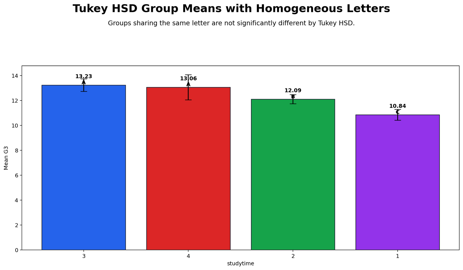
The group means chart shows a clear upward pattern from studytime group 1 to the higher studytime groups. Group 1 has the lowest mean, group 2 is higher, and groups 3 and 4 are the highest. The sample sizes are unequal, with group 4 much smaller than groups 1 and 2, which is why Tukey-Kramer pair-specific standard errors are important.
The letters summarize the post hoc grouping visually. The main interpretation is that the low studytime group is separated from the higher-performing groups, while the two highest means are close to each other. The chart should be read together with the pairwise table because compact letters are a summary, while the pairwise table gives the exact adjusted p-values and confidence intervals.
Python Chart 3: Tukey q Statistic Ranking
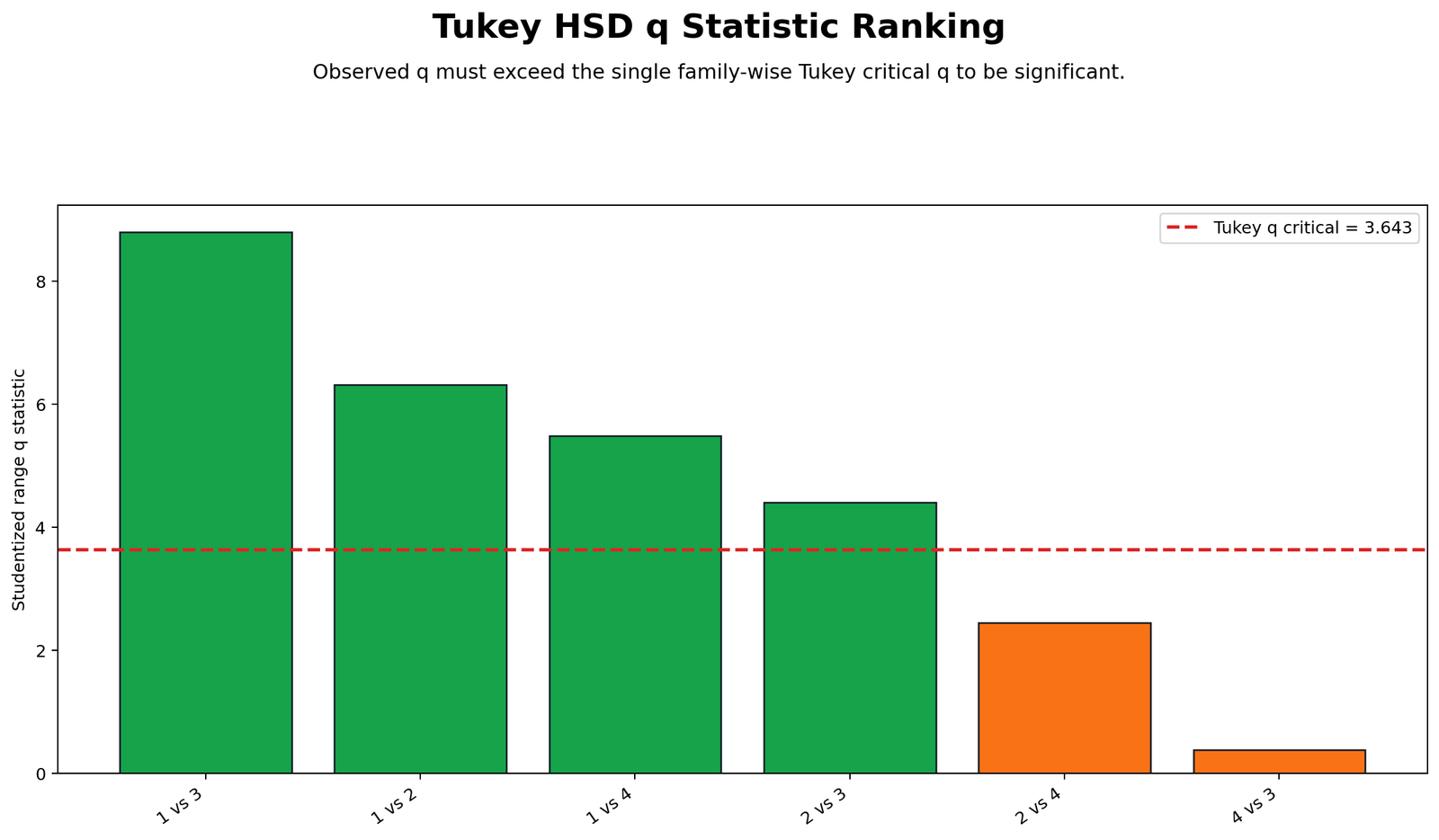
The q statistic ranking chart compares each observed q value with the Tukey critical q value. The strongest comparison is studytime 1 versus studytime 3, with q = 8.796. Studytime 1 versus 2, studytime 1 versus 4, and studytime 2 versus 3 also exceed the critical value of 3.643.
Studytime 2 versus 4 and studytime 4 versus 3 fall below the critical q line. This explains why those two comparisons are not significant even though their raw mean differences are not exactly zero. In Tukey HSD, the question is whether the difference is large enough relative to the familywise critical threshold.
Python Chart 4: Mean Difference Versus HSD Threshold
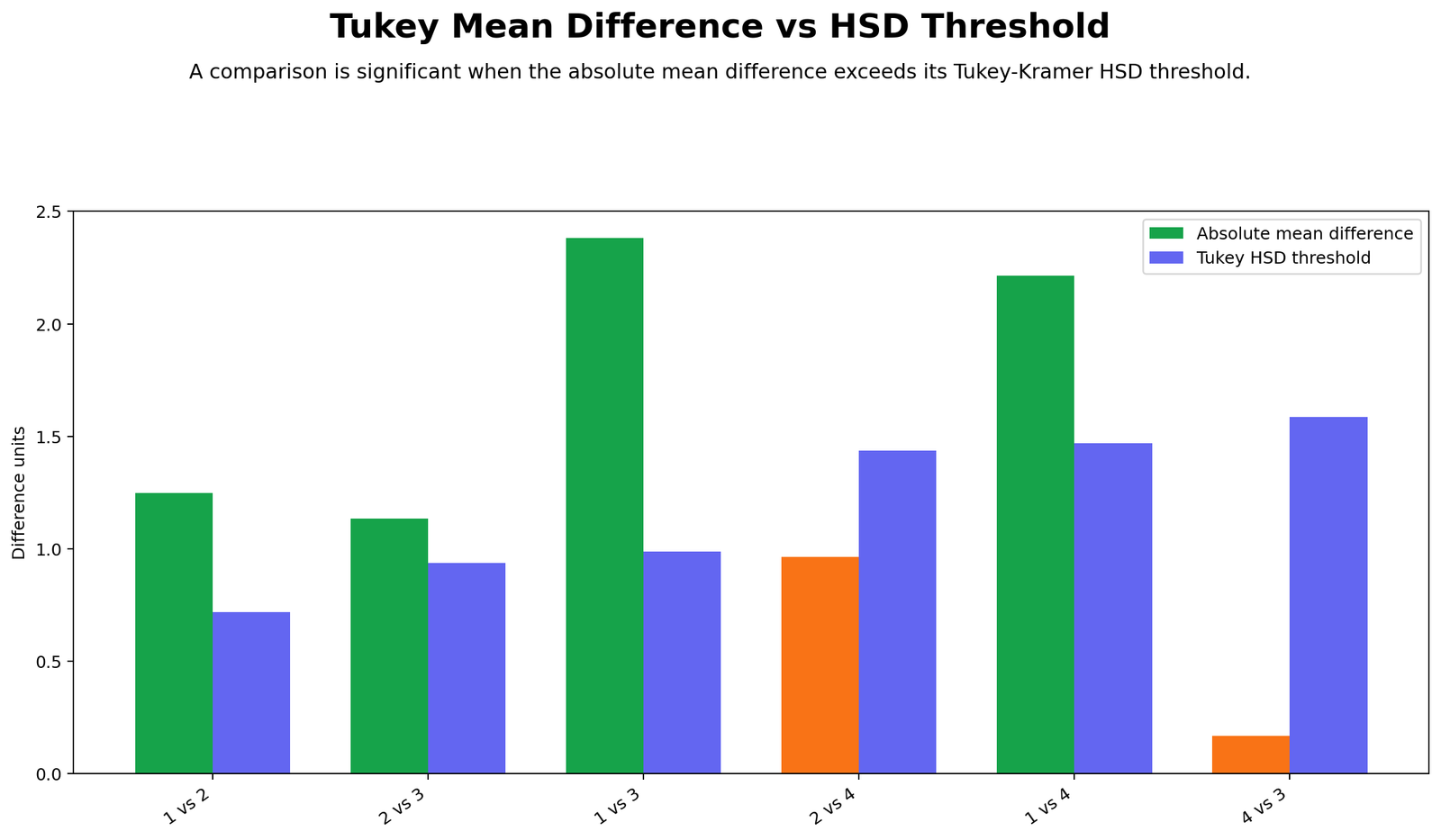
This chart compares the observed mean difference for each pair with the required Tukey-Kramer threshold. Because the sample sizes are unequal, the threshold changes by pair. Pairs involving group 4 often have wider thresholds because group 4 has only 35 observations.
The significant comparisons are the pairs where the observed difference is larger than the HSD threshold. The non-significant group 2 versus group 4 comparison has a mean difference of about 0.965, which is below its threshold of about 1.436. The group 4 versus group 3 comparison has an even smaller difference, about 0.170, far below its threshold.
Python Chart 5: Tukey Pairwise Decision Matrix
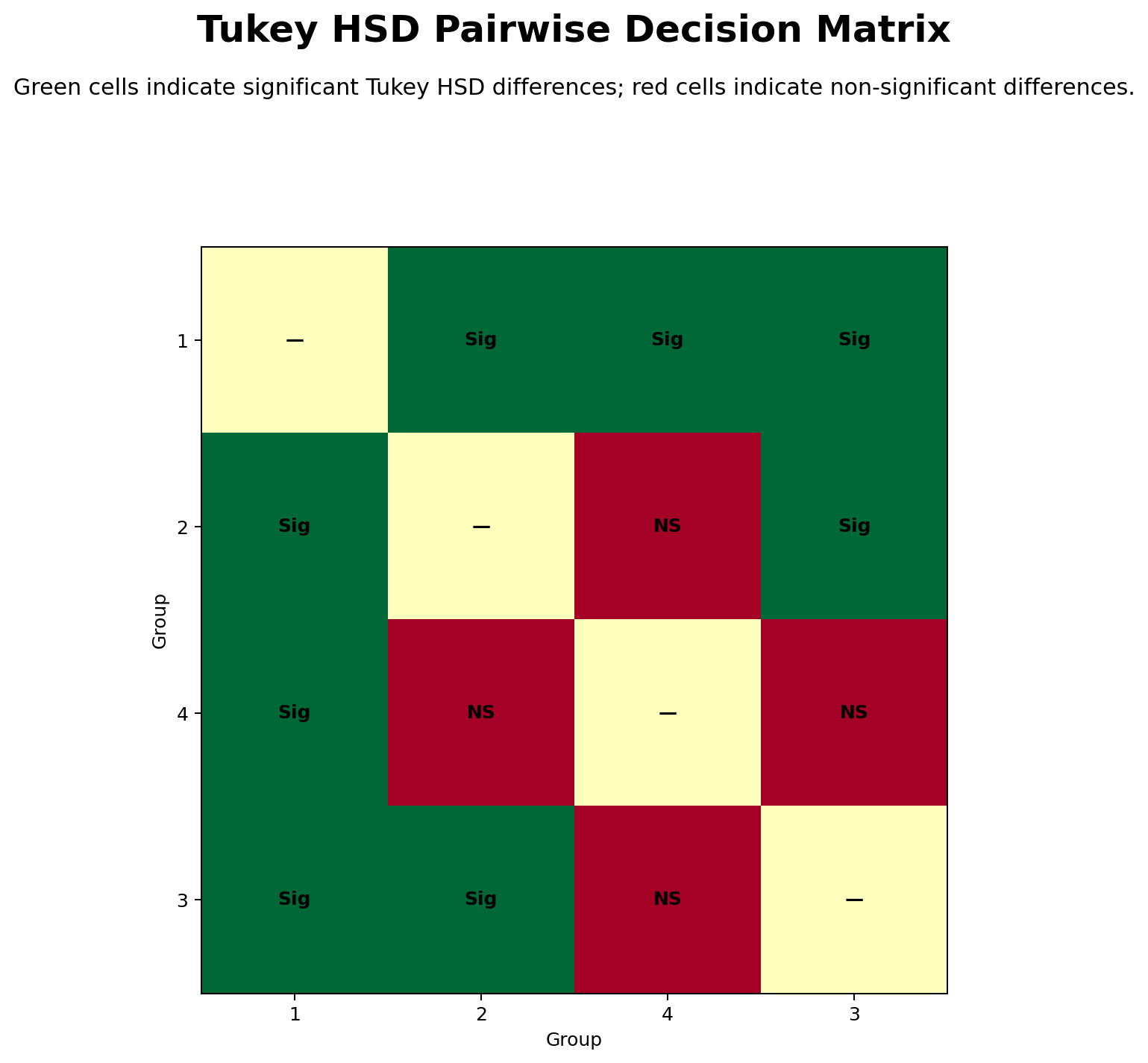
The decision matrix turns the pairwise table into a quick significance map. Significant cells show where Tukey HSD rejected equal means. The matrix highlights that studytime group 1 differs from all other groups and that group 2 differs from group 3.
The matrix also prevents overstatement. It shows that group 2 and group 4 are not significantly different and that group 3 and group 4 are not significantly different. This is important because a simple line chart of means might tempt readers to rank every group as significantly different, which is not supported by the Tukey result.
Python Chart 6: Tukey Adjusted p-values
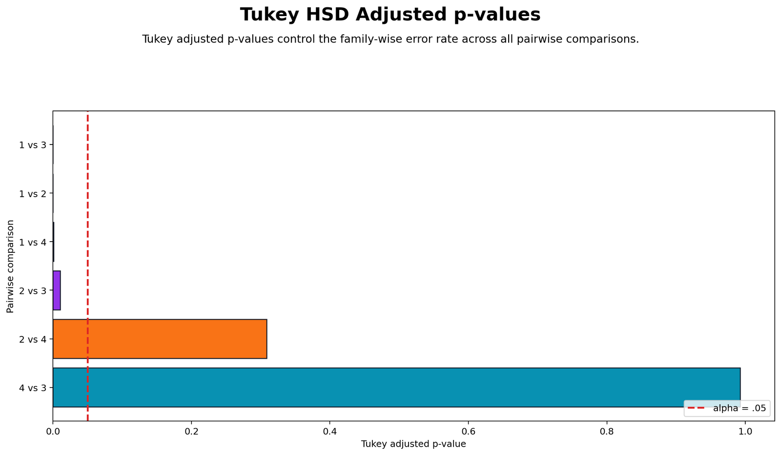
The adjusted p-value chart shows which comparisons stay below the .05 line after Tukey adjustment. Studytime 1 versus 3 has the smallest adjusted p-value, followed by studytime 1 versus 2, studytime 1 versus 4, and studytime 2 versus 3. These are the four significant comparisons.
The non-significant comparisons have much larger adjusted p-values: studytime 2 versus 4 is about .308, and studytime 4 versus 3 is about .993. These high values show that the observed differences are not strong enough after familywise adjustment.
Python Chart 7: ANOVA Variance Decomposition
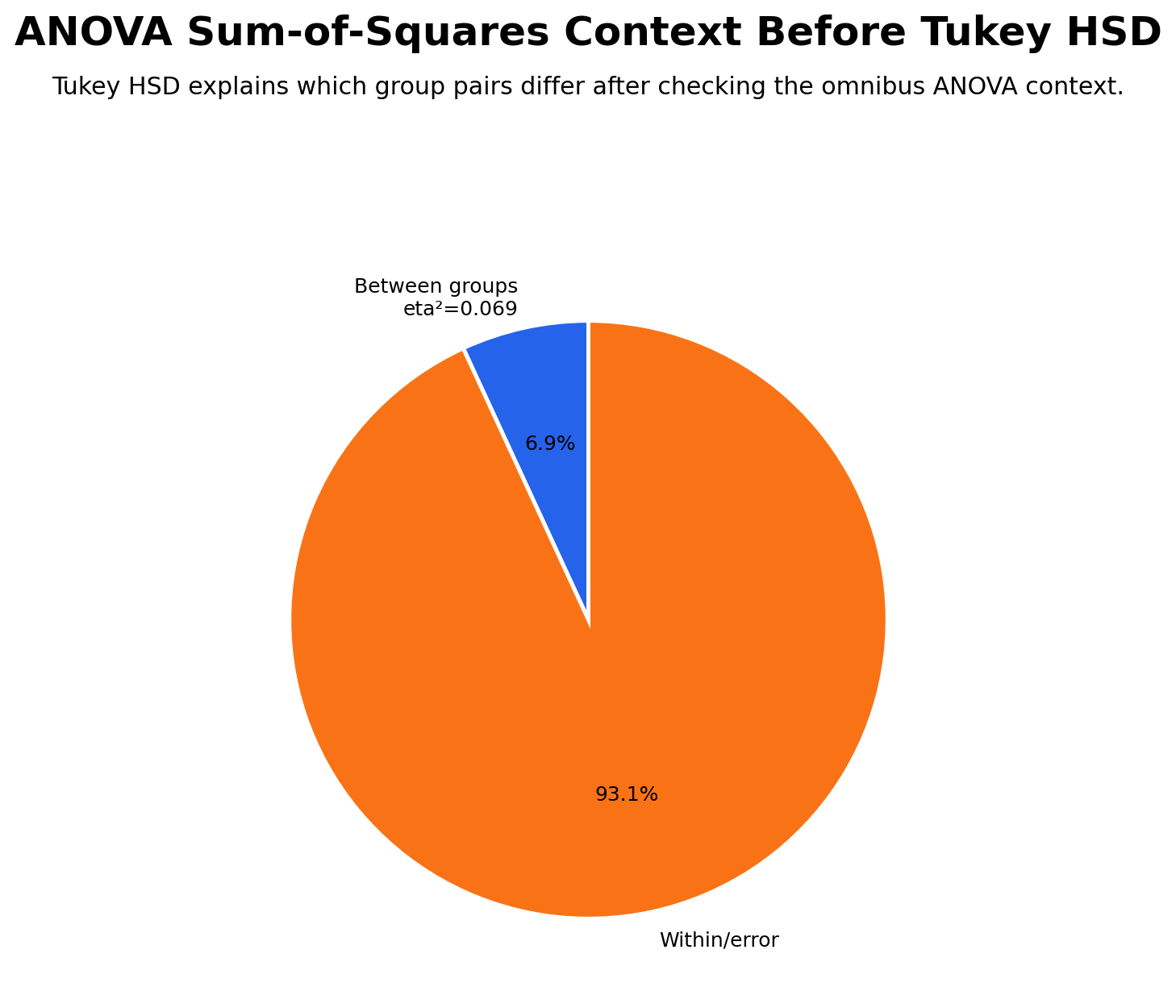
The ANOVA variance decomposition chart explains why the Tukey HSD test was needed. The between-group component is large enough relative to the within-group error to produce F = 15.876 and p < .001. This means the studytime group means are not all equal.
The chart also shows that much variation remains within the groups. Eta squared is about .069, so the studytime factor explains a meaningful but not overwhelming part of the final grade variation. Tukey HSD then identifies which specific pairs contribute to that overall ANOVA result.
Python Chart 8: Distribution Context Violin and Box Plot
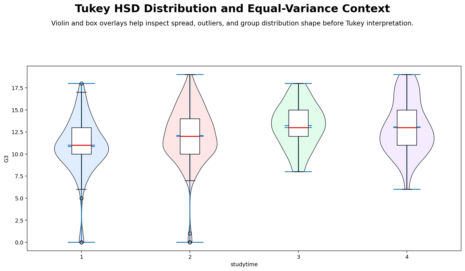
The distribution context chart shows why post hoc tests are interpreted with both means and spread. The higher studytime groups tend to have higher grade distributions, but the distributions still overlap. This overlap is normal in real data and explains why not every pairwise difference becomes statistically significant.
The group 1 distribution sits lower overall, which supports the significant differences involving group 1. Groups 3 and 4 appear close in central tendency, which supports the non-significant Tukey comparison between them. This chart gives practical context to the numerical Tukey table.
R Chart-by-Chart Validation
The R charts validate the same Tukey HSD interpretation using a separate workflow. The R output confirms the ANOVA result, equal-variance context, group means, q statistics, adjusted p-values and pairwise decisions.
R Chart 1: Tukey HSD Simultaneous Confidence Interval Forest
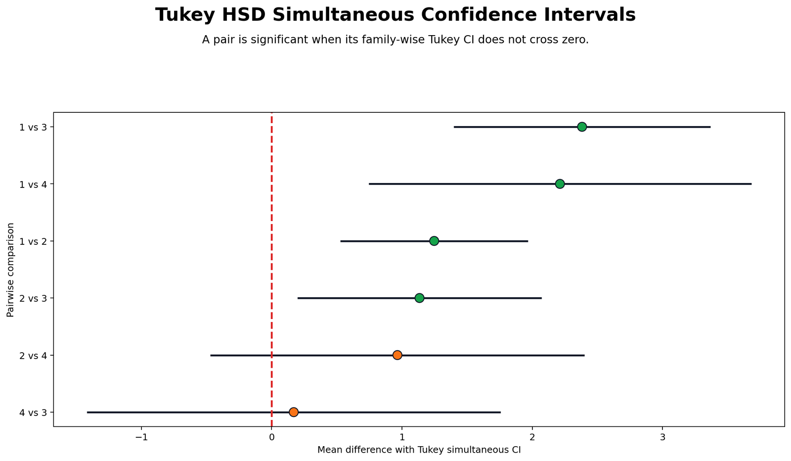
The R confidence interval forest repeats the same evidence as the Python chart. Four intervals exclude zero and two intervals include zero. This validates the conclusion that four pairwise differences are statistically significant after Tukey adjustment.
The R chart also makes the direction of the differences clear. Comparisons involving studytime group 1 show the largest reliable gaps, especially the comparison between group 1 and group 3.
R Chart 2: Group Means and Homogeneous Letters
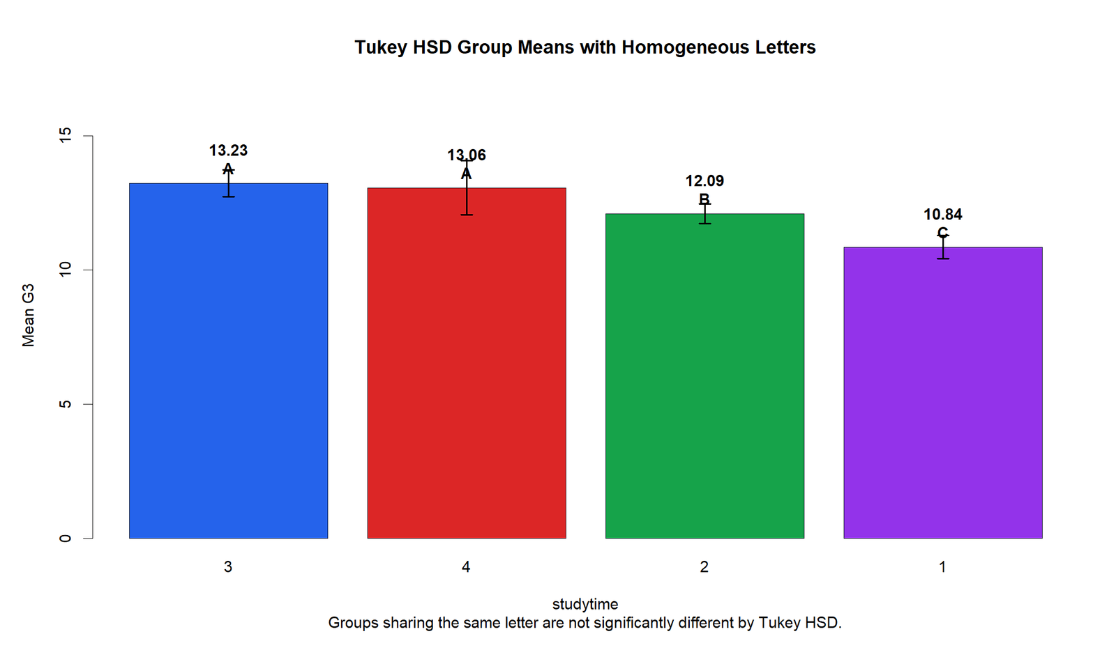
The R group means chart confirms the same pattern: group 1 has the lowest mean, group 2 is higher, and groups 3 and 4 are highest. The overall story is not simply “more studytime always means a separate mean.” The Tukey result shows where the statistically reliable gaps actually occur.
This chart is useful for readers who need a fast visual summary before reading the pairwise table. The chart should be paired with the adjusted p-value table for exact reporting.
R Chart 3: Tukey q Statistic Ranking
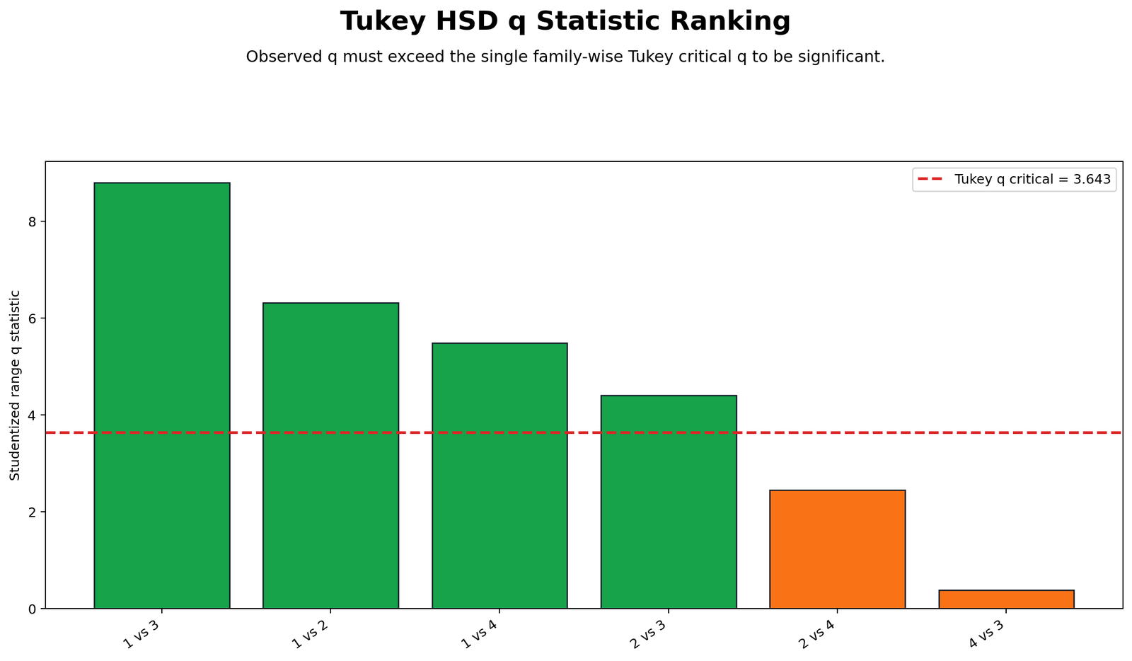
The R q statistic ranking validates that the significant pairs have q values above the critical value. The group 1 versus group 3 comparison is the strongest, while group 4 versus group 3 is the weakest.
The q chart is helpful because it connects the Tukey HSD decision to the Studentized range distribution instead of only showing p-values. It shows the actual test statistic logic behind the final decision.
R Chart 4: Mean Difference Versus HSD Threshold
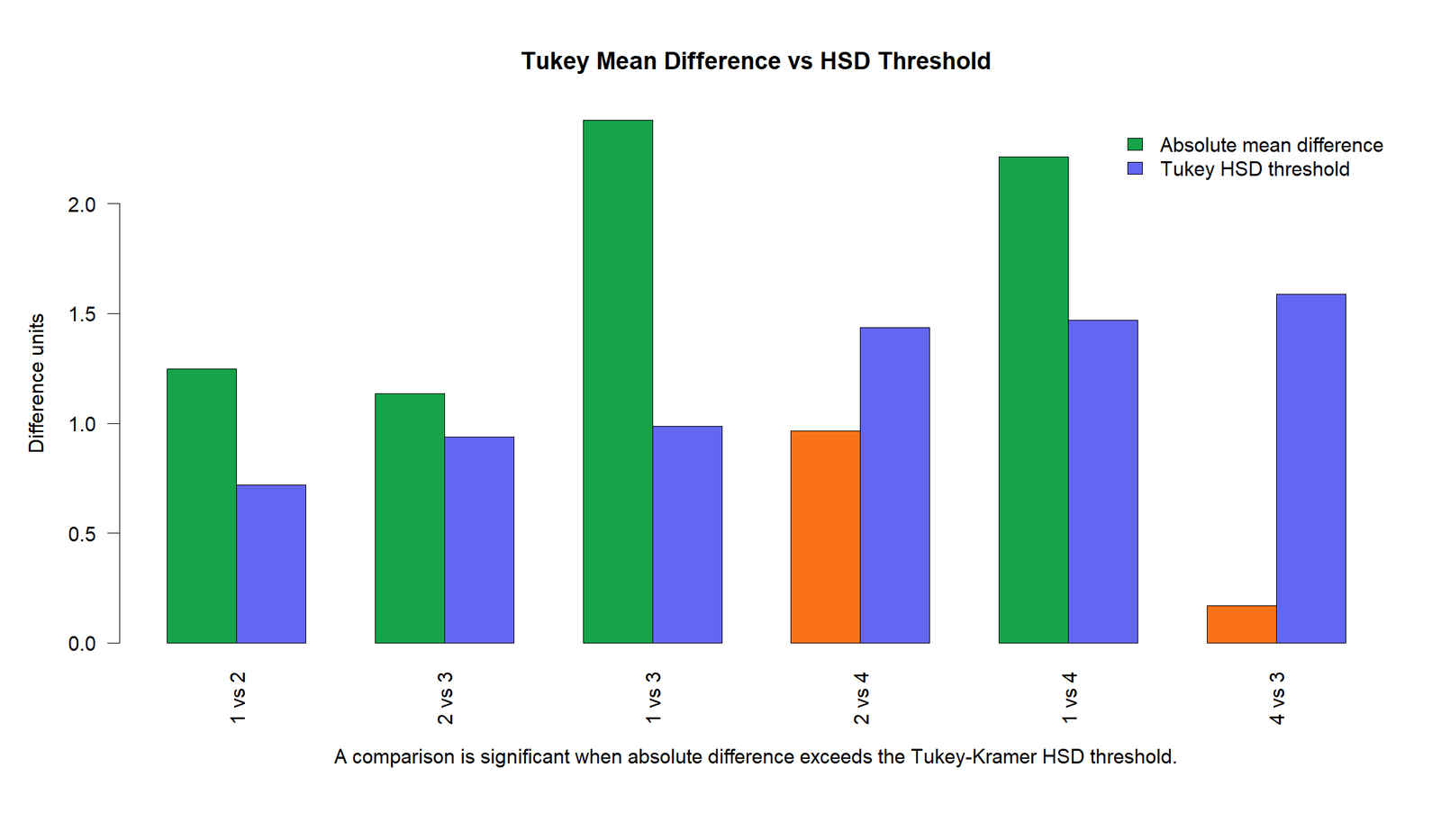
The R threshold chart confirms the unequal-sample-size logic. Pairs with smaller groups need a larger observed difference to become significant. This is one reason group 2 versus group 4 is not significant even though the raw mean difference is close to one grade point.
The threshold chart gives a practical teaching view of Tukey-Kramer. A pairwise mean difference is not interpreted alone; it is interpreted against its standard error and the familywise critical value.
R Chart 5: Pairwise Decision Matrix
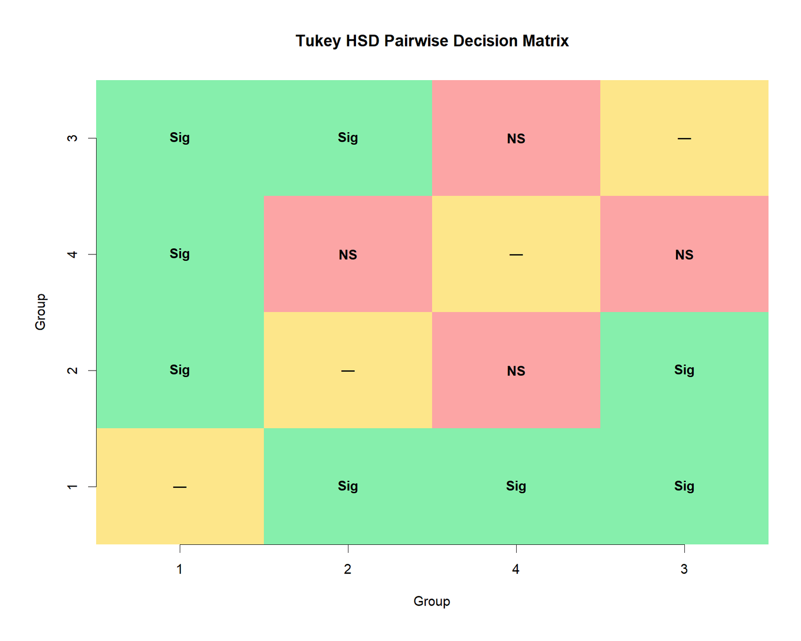
The R decision matrix matches the Python result. The significant structure is concentrated around group 1 and the group 2 versus group 3 comparison. The two non-significant comparisons remain group 2 versus group 4 and group 3 versus group 4.
This matrix is one of the easiest visuals for a final report because it prevents readers from missing a pair. Every possible comparison is represented in one compact chart.
R Chart 6: Adjusted p-values
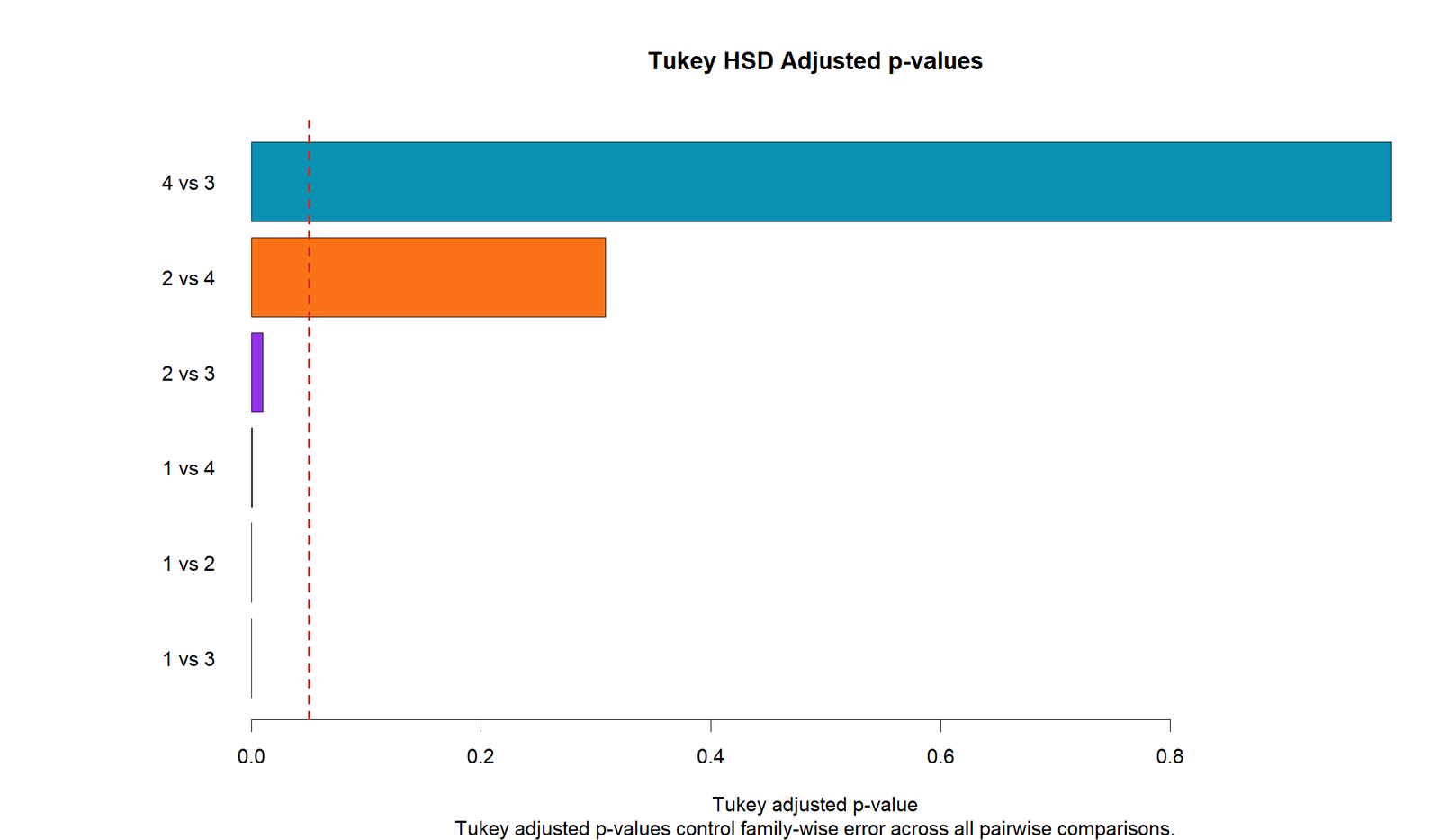
The R adjusted p-value chart validates the familywise corrected decisions. The four significant pairs are below .05, and the two non-significant pairs are above .05. This chart is useful when readers are more familiar with p-values than q statistics.
The adjusted p-values should be reported instead of unadjusted p-values because the entire purpose of Tukey HSD is to control error across the full set of pairwise comparisons.
R Chart 7: ANOVA Variance Decomposition
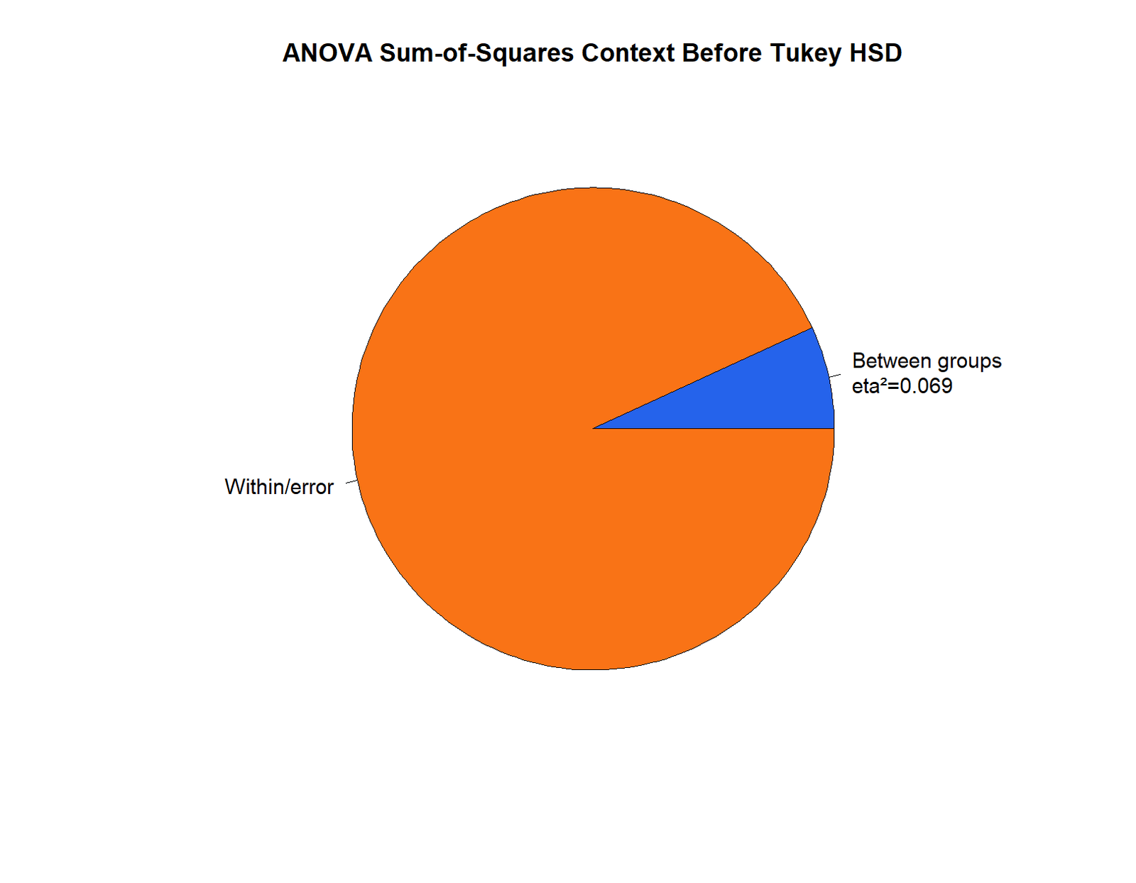
The R ANOVA variance chart confirms that the between-group studytime effect is statistically meaningful, but much of the grade variation remains within groups. This supports a balanced conclusion: studytime groups differ, but studytime is not the only factor related to final grade.
This is why post hoc interpretation should include effect size and descriptive context, not only p-values. The significant ANOVA opens the door to Tukey HSD, while the effect size explains practical magnitude.
R Chart 8: Distribution Context Violin and Box Plot
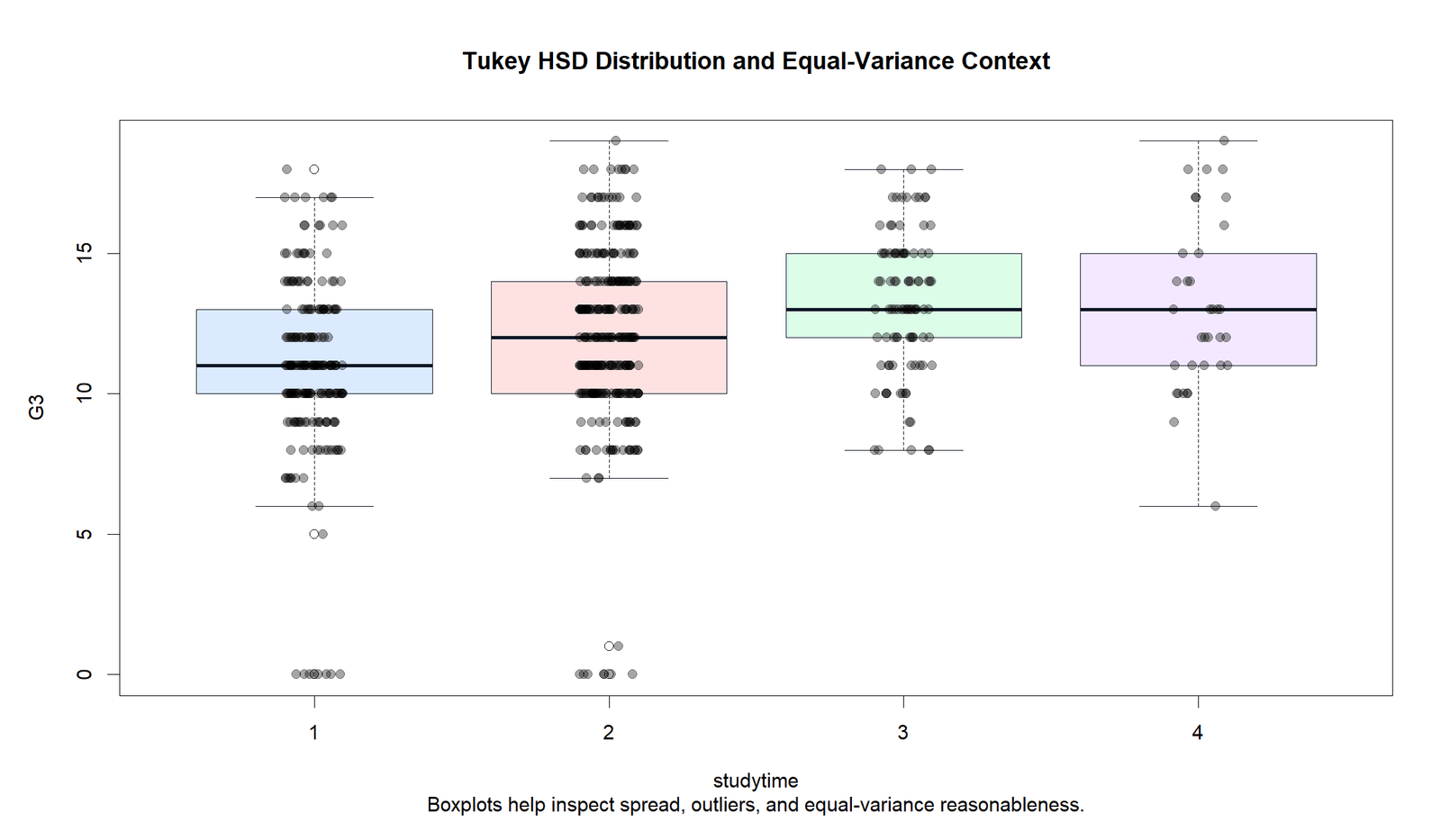
The R distribution chart confirms the Python distribution context. Group 1 is visibly lower, while groups 3 and 4 are close. This visual shape matches the Tukey result: group 1 differs from higher groups, but groups 3 and 4 do not differ significantly.
Distribution charts are important because they show overlap and spread. A significant Tukey result does not mean groups are completely separate; it means the difference between their means is large enough relative to the pooled error and familywise adjustment.
SPSS, R, Python and Excel Workflows for Tukey HSD Test
The Tukey HSD Test can be performed in SPSS, R, Python and Excel. The core workflow is the same in every tool: check the ANOVA model, review assumption context, run Tukey HSD or Tukey-Kramer comparisons, interpret adjusted p-values and simultaneous confidence intervals, then report the significant and non-significant pairs clearly.
SPSS Workflow
| Step | SPSS Menu or Syntax | Purpose |
|---|---|---|
| Open data | File > Open > Data | Load the dataset containing G3 and studytime. |
| Run one-way ANOVA | Analyze > Compare Means > One-Way ANOVA | Set G3 as dependent variable and studytime as factor. |
| Select Tukey | Post Hoc > Tukey | Request Tukey HSD pairwise comparisons. |
| Check homogeneity | Options > Homogeneity of variance test | Review whether equal-variance context is acceptable. |
| Interpret output | ANOVA, Multiple Comparisons, Homogeneous Subsets | Report significant pairs and adjusted p-values. |
R Workflow
| Step | R Function | Purpose |
|---|---|---|
| Read data | read.csv() | Load the dataset. |
| Convert factor | factor(studytime) | Ensure studytime is treated as a grouping variable. |
| Run ANOVA | aov(G3 ~ studytime) | Test overall mean differences. |
| Run Tukey HSD | TukeyHSD(model) | Get adjusted pairwise comparisons. |
| Plot results | plot(TukeyHSD(model)) | Visualize simultaneous confidence intervals. |
Python Workflow
| Step | Python Library | Purpose |
|---|---|---|
| Read data | pandas | Load and clean the dataset. |
| Run ANOVA | statsmodels | Fit one-way ANOVA and obtain MSE. |
| Run Tukey | statsmodels.stats.multicomp.pairwise_tukeyhsd | Calculate Tukey HSD comparisons. |
| Validate q logic | scipy.stats.studentized_range | Calculate q critical value and Tukey-Kramer thresholds. |
| Create charts | matplotlib | Build confidence interval, p-value and decision visuals. |
Excel Workflow
| Excel Task | Tool or Formula | Purpose |
|---|---|---|
| Run ANOVA | Data Analysis ToolPak > ANOVA: Single Factor | Get group means, sample sizes and MSE. |
| Find q critical | Studentized range table or external calculator | Use alpha, number of groups and error df. |
| Calculate pair SE | =SQRT((MSE/2)*(1/n1+1/n2)) | Apply Tukey-Kramer unequal-n denominator. |
| Calculate q | =ABS(mean1-mean2)/SE | Compute Tukey q statistic. |
| Decision | =IF(q>qcrit,"Significant","Not significant") | Classify each pairwise comparison. |
Code Blocks for Tukey HSD Test
SPSS Syntax for Tukey HSD Test
* Tukey HSD Test / Tukey-Kramer Post Hoc Analysis.
* Dependent variable: G3.
* Factor variable: studytime.

TITLE "Tukey HSD Test / Tukey-Kramer Post Hoc Analysis".

ONEWAY G3 BY studytime
  /STATISTICS DESCRIPTIVES HOMOGENEITY WELCH BROWNFORSYTHE
  /PLOT MEANS
  /MISSING ANALYSIS
  /POSTHOC=TUKEY ALPHA(0.05).

OUTPUT EXPORT
  /CONTENTS EXPORT=ALL
  /PDF DOCUMENTFILE="D:\DATA ANALYSIS\F Post Hoc Tests\Tukey HSD Test\SPSS_Output\pdf\Tukey-HSD-Test-SPSS-Output.pdf".
R Code for Tukey HSD Test
# Tukey HSD Test in R
data <- read.csv("dataset.csv")

data$studytime <- factor(
  data$studytime,
  levels = c(1, 2, 3, 4),
  labels = c("Studytime 1: <2 hours",
             "Studytime 2: 2 to 5 hours",
             "Studytime 3: 5 to 10 hours",
             "Studytime 4: >10 hours")
)

model <- aov(G3 ~ studytime, data = data)
summary(model)

tukey_result <- TukeyHSD(model, "studytime", conf.level = 0.95)
print(tukey_result)

plot(tukey_result, las = 1)
Python Code for Tukey HSD Test
# Tukey HSD Test in Python
import pandas as pd
import statsmodels.api as sm
from statsmodels.formula.api import ols
from statsmodels.stats.multicomp import pairwise_tukeyhsd

df = pd.read_csv("dataset.csv")
df = df.dropna(subset=["G3", "studytime"])

model = ols("G3 ~ C(studytime)", data=df).fit()
anova_table = sm.stats.anova_lm(model, typ=2)
print(anova_table)

tukey = pairwise_tukeyhsd(
    endog=df["G3"],
    groups=df["studytime"],
    alpha=0.05
)
print(tukey)
Excel Formula Logic for Tukey-Kramer
Pair Standard Error:
=SQRT(($MSE$/2)*(1/n_i + 1/n_j))

q Statistic:
=ABS(mean_i - mean_j) / pair_standard_error

Decision:
=IF(q_statistic > q_critical, "Significant", "Not significant")

Simultaneous CI:
Lower = mean_difference - q_critical * pair_standard_error
Upper = mean_difference + q_critical * pair_standard_error
APA Reporting Wording for Tukey HSD Test
A one-way ANOVA was conducted to compare final grade scores across four studytime groups. The ANOVA was statistically significant, F(3, 645) = 15.876, p < .001, η² = .069. The homogeneity of variance context did not show a serious violation, with the median-centered Levene / Brown-Forsythe result p = .380.
Tukey HSD post hoc comparisons showed that students in studytime group 1 had significantly lower G3 scores than students in group 2, MD = 1.247, p < .001, group 3, MD = 2.382, p < .001, and group 4, MD = 2.213, p = .001. Studytime group 2 was also significantly lower than group 3, MD = 1.135, p = .010. The differences between group 2 and group 4 and between group 3 and group 4 were not statistically significant.
Short report sentence: Tukey HSD indicated that the lowest studytime group scored significantly lower than the higher studytime groups, while the two highest studytime groups did not differ significantly from each other.
Common Mistakes When Interpreting Tukey HSD
| Mistake | Why It Is a Problem | Correct Practice |
|---|---|---|
| Running many unadjusted t tests instead of Tukey HSD | Inflates familywise Type I error. | Use Tukey HSD when comparing all pairs after ANOVA. |
| Ignoring the omnibus ANOVA | Post hoc tests need ANOVA context. | Report ANOVA first, then Tukey results. |
| Reporting only p-values | P-values do not show effect size or direction clearly. | Report mean differences and simultaneous confidence intervals. |
| Assuming all ordered means are significantly different | Visible mean ranking does not equal statistical significance. | Check each pairwise Tukey comparison. |
| Using Tukey HSD when variances are clearly unequal | Tukey HSD assumes equal variance context. | Consider Games-Howell or Tamhane’s T2 when variance assumptions fail. |
Downloads and Resources for Tukey HSD Test
The reports below verify the ANOVA result, Tukey-Kramer pairwise comparisons, adjusted p-values, simultaneous confidence intervals, homogeneous subset summaries and software output used in this guide.
Download Python Report PDF
Python ANOVA, Tukey-Kramer pairwise results, q statistics and chart summary.
Download R Report PDF
R validation output for Tukey HSD, ANOVA context and pairwise comparisons.
Download SPSS Output PDF
SPSS output with descriptives, homogeneity tests, ANOVA and Tukey HSD tables.
External References
These external references are useful for readers who want additional mathematical or software documentation for Tukey HSD and the Studentized range distribution.
FAQs About Tukey HSD Test
What is the Tukey HSD Test used for?
The Tukey HSD Test is used after ANOVA to compare all pairs of group means while controlling the familywise error rate. It tells which specific groups differ after the overall ANOVA indicates that at least one group mean is different.
Is Tukey HSD the same as Tukey-Kramer?
Tukey HSD is the classic equal-sample-size form. Tukey-Kramer is the unequal-sample-size extension. In practical software output, Tukey HSD often uses Tukey-Kramer logic automatically when group sizes are unequal.
When is Tukey HSD significant?
A Tukey HSD comparison is significant when the adjusted p-value is below the chosen alpha level, usually .05. The same decision is supported when the simultaneous confidence interval excludes zero or when the q statistic exceeds the Tukey critical q value.
What did the Tukey HSD result show in this example?
The test showed 4 significant comparisons out of 6. Studytime group 1 was significantly lower than groups 2, 3 and 4. Studytime group 2 was significantly lower than group 3. The differences between groups 2 and 4 and between groups 3 and 4 were not significant.
Can I run Tukey HSD in Excel?
Excel’s Analysis ToolPak can run one-way ANOVA, but it does not provide a full Tukey HSD table automatically in the same way as SPSS, R or Python. You can calculate Tukey-Kramer manually in Excel using ANOVA MSE, group means, group sample sizes and a Studentized range critical value.
Should I use Tukey HSD if variances are unequal?
If variances are strongly unequal, Tukey HSD may not be the best choice. Consider Games-Howell or Tamhane’s T2 when equal variance assumptions are not reasonable.

