
Standard Scores, Standard Deviation Bands and Outlier Screening
Z Score: Formula, Interpretation, SPSS, Python, R and Excel Guide
Z Score analysis converts raw values into standard deviation units so every observation can be interpreted relative to the sample mean. In this guide, Z Score is explained with the formula, verified SPSS output, Python charts, R validation charts, Excel formulas, software workflows, APA reporting wording, and practical guidance for identifying ordinary, unusual, and extreme values.
Quick Answer: What Does a Z Score Show?
A Z Score tells how far a value is from the mean in standard deviation units. A Z Score of 0 means the value is exactly at the mean. A Z Score of +1 means the value is one standard deviation above the mean. A Z Score of -1 means the value is one standard deviation below the mean. A large absolute Z Score, such as |z| > 2 or |z| > 3, can flag unusual or extreme observations for review.
In this worked example, the main variable is G3 final grade. The verified SPSS output shows N = 649, mean = 11.91, standard deviation = 3.231, and the standardized variable z_G3 has mean approximately 0.00000 and standard deviation exactly 1.000000. The lowest G3 Z Score is -3.685, and the highest G3 Z Score is 2.196. This means the most distant G3 observations are on the lower-score side.
Final result: The Z Score transformation worked correctly because the standardized G3 variable has a mean of approximately 0 and a standard deviation of 1. For G3, 19 cases were beyond |z| > 2, and 16 cases were beyond |z| > 3. These cases should be reviewed as unusually distant or extreme values, especially because the largest negative Z Score values come from very low final grades.
Important reporting note: A Z Score is not automatically a hypothesis test. It is a standardized distance measure. However, a hypothesis-style screening rule can be used for clarity: the null screening statement says a case is not unusually distant from the mean, while the alternative screening statement says the case is unusually distant because its absolute Z Score exceeds a chosen cutoff such as 2 or 3.
Table of Contents
- What Is a Z Score?
- Z Score Formula
- Hypothesis-Style Screening Rule for Z Score
- Dataset and Variables Used
- Verified SPSS Output Interpretation
- Python Chart-by-Chart Interpretation
- R Chart-by-Chart Validation
- SPSS, R, Python and Excel Workflows
- Code Blocks for Z Score
- APA Reporting Wording
- Common Mistakes
- When to Use Z Score
- Downloads and Resources
- Related Guides
- FAQs
What Is a Z Score?
A Z Score is a standardized score that shows how many standard deviations a raw value is above or below the mean. Instead of reading a raw score only in its original unit, a Z Score expresses the same value on a common scale where the mean is 0 and the standard deviation is 1.
For example, a raw G3 final grade of 15 is easier to interpret after standardization. If the G3 mean is about 11.91 and the standard deviation is about 3.23, then a score of 15 is roughly one standard deviation above the mean. The Z Score makes that relationship explicit. A score of 0, on the other hand, is far below the mean and receives a large negative Z Score.
The Z Score is useful because it allows different variables to be compared on the same scale. G3 is measured in grade points from 0 to 19, age is measured in years from 15 to 22, and absences are measured as count values from 0 to 32. Their raw units are different, but their Z Score values are directly comparable as standardized distances from each variable’s own mean.
Plain-language meaning: A Z Score answers this question: “How far is this value from the average, measured in standard deviation units?” Positive values are above the mean, negative values are below the mean, and values near zero are close to average.
Z Score Formula
The standard Z Score formula is:
In symbols, the formula is often written as:
z = (x - x̄) / sWhere x is the raw value, x̄ is the sample mean, and s is the sample standard deviation. For a population version, the formula is written as:
z = (x - μ) / σWhere μ is the population mean and σ is the population standard deviation. In most practical data-analysis projects, the sample formula is used because the mean and standard deviation are calculated from the sample data.
| Z Score value | Meaning | Common interpretation |
|---|---|---|
| z = 0 | The value equals the mean. | Average or central value. |
| z = +1 | The value is one standard deviation above the mean. | Above average but not unusual. |
| z = -1 | The value is one standard deviation below the mean. | Below average but not unusual. |
| |z| > 2 | The value is more than two standard deviations from the mean. | Unusual value for review. |
| |z| > 3 | The value is more than three standard deviations from the mean. | Extreme value or possible outlier. |
Worked Z Score Example for G3
Using the verified SPSS values for G3, the mean is 11.91 and the standard deviation is 3.231. A student with G3 = 19 has the following approximate Z Score:
z = (19 - 11.91) / 3.231
z ≈ 2.196
This means a G3 score of 19 is about 2.20 standard deviations above the mean. A student with G3 = 0 has the following approximate Z Score:
z = (0 - 11.91) / 3.231
z ≈ -3.685
This means a G3 score of 0 is about 3.69 standard deviations below the mean. That is why the most distant G3 cases in this analysis appear on the negative side.
Hypothesis-Style Screening Rule for Z Score
A Z Score is not a full inferential test by itself, but it can be used with a hypothesis-style screening decision. This is useful when you want clear reporting language for unusual or extreme observations.
| Screening statement | Rule | Meaning |
|---|---|---|
| Null screening statement | H0: |z| ≤ cutoff | The case is not unusually distant from the mean based on the selected Z Score cutoff. |
| Alternative screening statement | H1: |z| > cutoff | The case is unusually distant from the mean and should be reviewed. |
| Unusual cutoff | |z| > 2 | The case is more than two standard deviations away from the mean. |
| Extreme cutoff | |z| > 3 | The case is more than three standard deviations away from the mean. |
Screening decision for G3: The SPSS output shows 19 cases with |z_G3| > 2 and 16 cases with |z_G3| > 3. Therefore, the ordinary-value screening statement is rejected for those cases. They should be reviewed as unusual or extreme G3 observations, especially because several of the most distant cases are very low final grades.
Important caution: Do not delete cases only because their Z Score is large. A large Z Score flags a case for review. The analyst must still decide whether the value is a data-entry error, a meaningful extreme observation, a legitimate rare outcome, or a value that requires robust analysis.
Dataset and Variables Used
This Z Score guide uses the student performance dataset. The main outcome variable is G3 final grade. Additional numeric variables were standardized to show how Z Score values can compare unusual and extreme values across variables with different raw scales.
| Item | Value | Purpose in Z Score Analysis |
|---|---|---|
| Main variable | G3 final grade | Used to demonstrate raw distribution, standardized distribution, z-score bands, and most distant cases. |
| Additional variables | G1, G2, age, absences | Used to compare unusual and extreme observations across variables. |
| Valid N | 649 | All cases were available in the verified SPSS output. |
| Standardized variables | z_G1, z_G2, z_G3, z_age, z_absences | SPSS generated standardized variables with mean 0 and standard deviation 1. |
| Outlier screening cutoffs | |z| > 2 and |z| > 3 | Used to identify unusual and extreme standardized values. |
The analysis uses Z Score values for descriptive screening and standardization. It does not claim that every extreme Z Score is an error. Instead, the goal is to locate observations far from the mean and interpret them with charts, frequency tables, and context.
Verified SPSS Output Interpretation for Z Score
The SPSS output confirms that the Z Score variables were created correctly. The raw variables have their original means and standard deviations, while the standardized variables have mean approximately 0 and standard deviation 1.
SPSS Descriptive Statistics
| Variable | N | Minimum | Maximum | Mean | Standard Deviation | Interpretation |
|---|---|---|---|---|---|---|
| G1 | 649 | 0 | 19 | 11.40 | 2.745 | Raw first-period grade scale. |
| G2 | 649 | 0 | 19 | 11.57 | 2.914 | Raw second-period grade scale. |
| G3 | 649 | 0 | 19 | 11.91 | 3.231 | Main final-grade variable for Z Score interpretation. |
| age | 649 | 15 | 22 | 16.74 | 1.218 | Raw age variable with narrow spread. |
| absences | 649 | 0 | 32 | 3.66 | 4.641 | Raw count variable with wider right-side spread. |
SPSS Standardized Variables
| Standardized Variable | N | Minimum Z Score | Maximum Z Score | Mean | Standard Deviation | Interpretation |
|---|---|---|---|---|---|---|
| z_G1 | 649 | -4.152 | 2.769 | 0.00000 | 1.000000 | G1 standardized correctly; some very low G1 values are far below the mean. |
| z_G2 | 649 | -3.971 | 2.550 | 0.00000 | 1.000000 | G2 standardized correctly; low values are more distant than high values. |
| z_G3 | 649 | -3.685 | 2.196 | 0.00000 | 1.000000 | Main standardized final-grade variable. |
| z_age | 649 | -1.432 | 4.315 | 0.00000 | 1.000000 | Older age values are far above the age mean because the age range is narrow. |
| z_absences | 649 | -0.789 | 6.107 | 0.00000 | 1.000000 | High absence counts create very large positive Z Score values. |
G3 Z Score Flag Counts
| Flag Rule | Not Flagged | Flagged | Flagged Percent | Interpretation |
|---|---|---|---|---|
| |z_G3| > 2 | 630 | 19 | 2.9% | These cases are unusual because they are more than two standard deviations from the G3 mean. |
| |z_G3| > 3 | 633 | 16 | 2.5% | These cases are extreme because they are more than three standard deviations from the G3 mean. |
G3 Z Score Band Table
| Z Score Band | Frequency | Percent | Cumulative Percent | Interpretation |
|---|---|---|---|---|
| below -3 | 16 | 2.5% | 2.5% | Extreme low G3 values. |
| -3 to -2 | 1 | 0.2% | 2.6% | Unusual low G3 value. |
| -2 to -1 | 48 | 7.4% | 10.0% | Below-average G3 values but not extreme. |
| -1 to 0 | 236 | 36.4% | 46.4% | Ordinary values slightly below the mean. |
| 0 to 1 | 266 | 41.0% | 87.4% | Ordinary values slightly above the mean. |
| 1 to 2 | 80 | 12.3% | 99.7% | Above-average values, mostly still ordinary. |
| 2 to 3 | 2 | 0.3% | 100.0% | Unusual high G3 values. |
| above 3 | 0 | 0.0% | 100.0% | No G3 cases exceed three standard deviations above the mean. |
SPSS Explore Output for z_G3
| Statistic | z_G3 Value | Interpretation |
|---|---|---|
| Mean | 0.00000 | The standardized mean is centered at zero. |
| 95% CI for Mean | -0.07708 to 0.07708 | The standardized mean is very close to zero. |
| Median | 0.02909 | The median is also close to zero. |
| Variance | 1.000 | The standardized variance is 1. |
| Standard Deviation | 1.000000 | The standardized standard deviation is 1. |
| Minimum | -3.685 | The most extreme low G3 value is 3.685 standard deviations below the mean. |
| Maximum | 2.196 | The most extreme high G3 value is 2.196 standard deviations above the mean. |
| Range | 5.881 | The full standardized spread from minimum to maximum is 5.881 Z Score units. |
| Interquartile Range | 1.238 | The middle half of standardized G3 values spans about 1.238 Z Score units. |
| Skewness | -0.913 | The standardized distribution remains left-skewed because standardization does not change shape. |
| Kurtosis | 2.712 | The standardized distribution retains the same tail-shape pattern as raw G3. |
Group Z Score Summary by Sex
| Sex Group | N | Mean z_G3 | Standard Deviation | Interpretation |
|---|---|---|---|---|
| Female | 383 | 0.10749 | 0.967032 | Female group mean is slightly above the overall G3 mean. |
| Male | 266 | -0.15477 | 1.027869 | Male group mean is slightly below the overall G3 mean. |
| Total | 649 | 0.00000 | 1.000000 | The total standardized distribution remains centered at zero. |
SPSS interpretation summary: SPSS confirms that Z Score standardization worked correctly. Each standardized variable has mean 0.00000 and standard deviation 1.000000. For G3, the lower tail is more extreme than the upper tail because the minimum Z Score is -3.685, while the maximum is 2.196. The G3 band table shows that most students fall between -1 and +1, while 19 cases exceed |z| > 2 and 16 cases exceed |z| > 3.
Python Chart-by-Chart Interpretation
The Python charts explain the Z Score result visually. The first two charts compare raw and standardized distributions. The next charts show standardized bands, unusual and extreme counts, most distant cases, and group mean Z Score differences.
Python Chart 1: Raw Distribution with Standard Deviation Bands
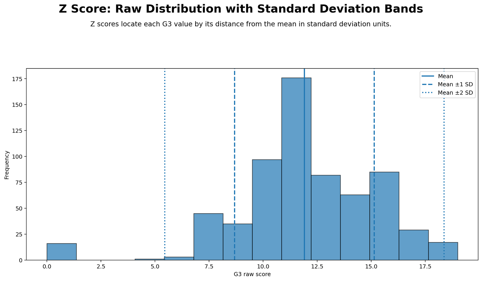
This chart begins with the raw G3 scale. The center line marks the mean, which is about 11.91. The dashed lines show approximately one standard deviation below and above the mean, and the dotted lines show approximately two standard deviations below and above the mean. The chart makes the Z Score idea easier to understand because each band corresponds to a standardized distance. A G3 value near the mean has a Z Score close to 0. A value around one dashed-line distance above the mean has a Z Score near +1, and a value around one dashed-line distance below the mean has a Z Score near -1.
The raw histogram shows that most G3 scores fall between the -1 SD and +1 SD region. The low score values near 0 are far to the left and fall beyond the -2 SD band. This explains why the minimum G3 Z Score is -3.685. The upper side extends to 19, but it does not reach beyond +3 standard deviations. Therefore, the raw distribution chart supports the SPSS finding that the most extreme G3 values are on the lower side.
Python Chart 2: Standardized Z Score Distribution
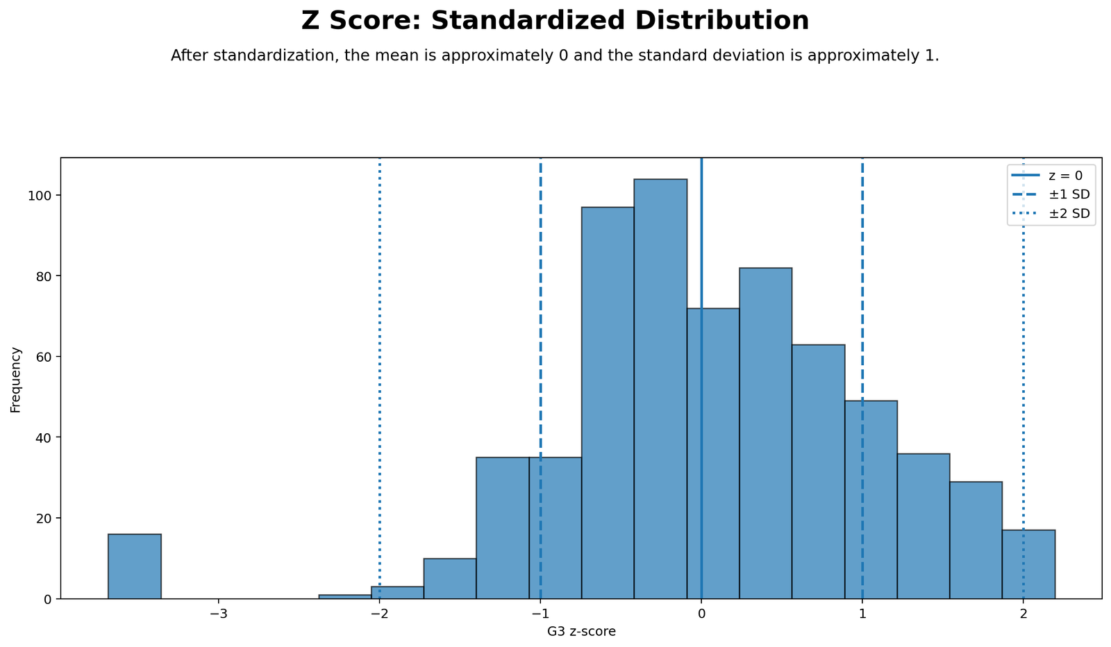
This chart shows the same G3 values after standardization. The x-axis is no longer raw grade points; it is the G3 Z Score. The solid line at z = 0 is the standardized mean. The dashed lines at -1 and +1 show one standard deviation below and above the mean. The dotted lines at -2 and +2 show two standard deviations below and above the mean.
The standardized distribution confirms that the Z Score transformation worked correctly. The mean is approximately 0 and the standard deviation is approximately 1. However, the shape of the distribution does not become normal simply because the values were standardized. The left tail remains visible, and a small group of cases appears below z = -3. This is an important lesson: Z Score standardization changes the scale, but it does not remove skewness, kurtosis, or outliers.
Python Chart 3: Cases by Standardized Band

This chart summarizes how many G3 cases fall into each Z Score band. The largest groups are from -1 to 0 and 0 to 1. Specifically, 36.4% of cases fall between -1 and 0, while 41.0% fall between 0 and 1. Together, most students fall within one standard deviation of the G3 mean.
The chart also shows the unusual and extreme regions. About 7.4% of cases fall between -2 and -1, 2.5% fall below -3, 0.2% fall between -3 and -2, and 0.3% fall between 2 and 3. No cases appear above +3. The visual result agrees with the SPSS frequency table. The main standardized distribution is centered, but the lower tail contains the most extreme observations.
Python Chart 4: Unusual and Extreme Values by Variable
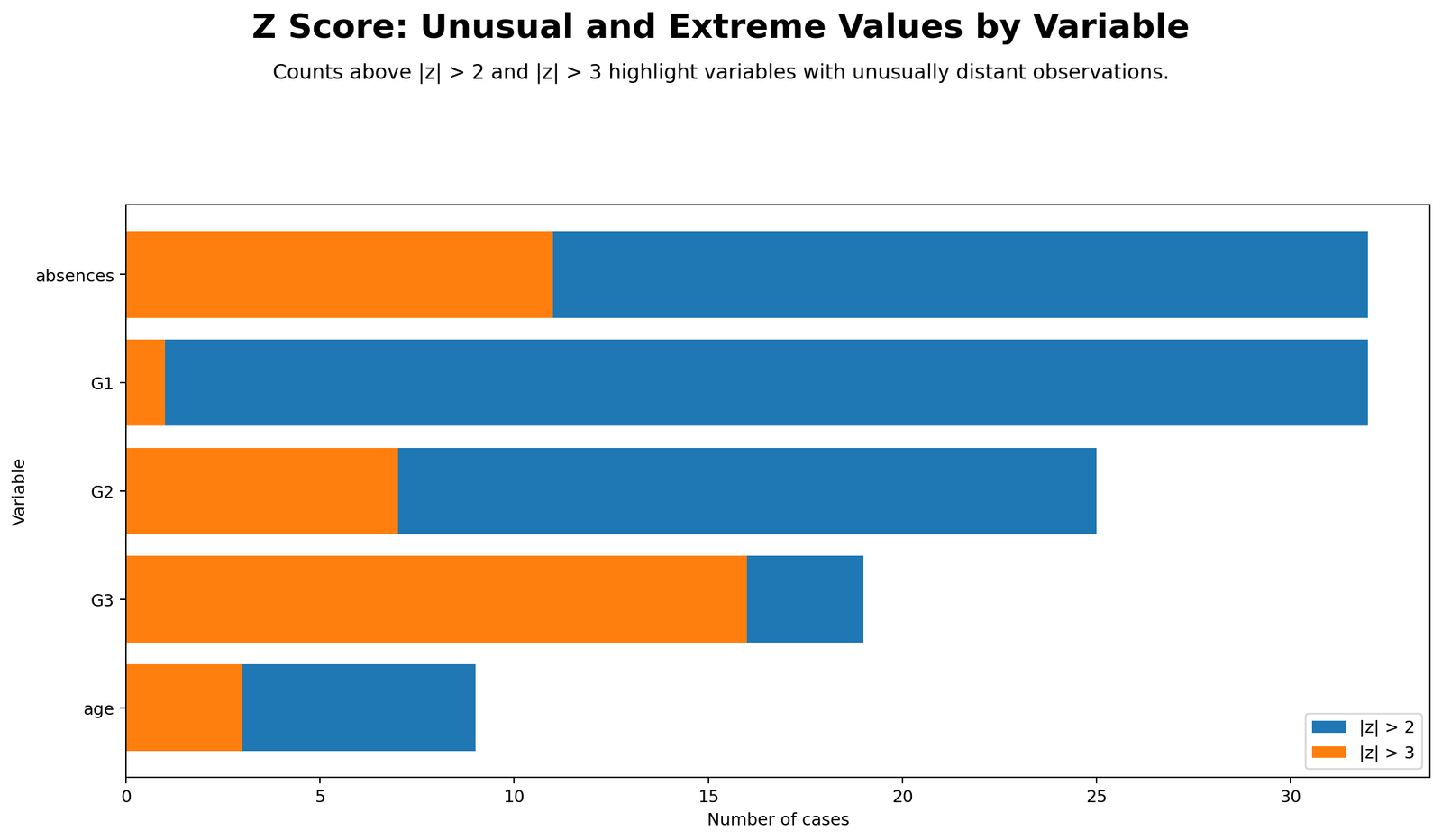
This chart compares unusual and extreme values across several variables. The blue bars represent |z| > 2, while the orange bars represent |z| > 3. This is one of the biggest strengths of Z Score standardization: it allows variables with different raw scales to be compared on the same standardized distance scale.
The chart shows that absences has the largest number of unusual values beyond |z| > 2, which makes sense because absences is a count variable with a long right tail. G1 and G2 also show many unusual values, mostly because low grade values are far below their means. G3 has 19 cases beyond |z| > 2 and 16 cases beyond |z| > 3. Age has fewer unusual cases, but the high end of age can still be distant because the age standard deviation is small.
Python Chart 5: Most Distant G3 Cases

This chart lists the most distant G3 cases by absolute Z Score. Most of the top cases are on the negative side, meaning they are far below the overall G3 mean. The vertical reference lines help separate ordinary, unusual, and extreme standardized values. Cases beyond -3 should be reviewed carefully because they are more than three standard deviations below the mean.
In practical reporting, the chart should not be used to automatically remove these cases. Instead, it should guide the analyst toward case review. A low G3 value may represent a real poor performance outcome, a withdrawal, a failed final grade, or a data-entry problem. The Z Score tells us that the case is distant; the dataset context tells us what that distance means.
Python Chart 6: Group Mean Standardized Score
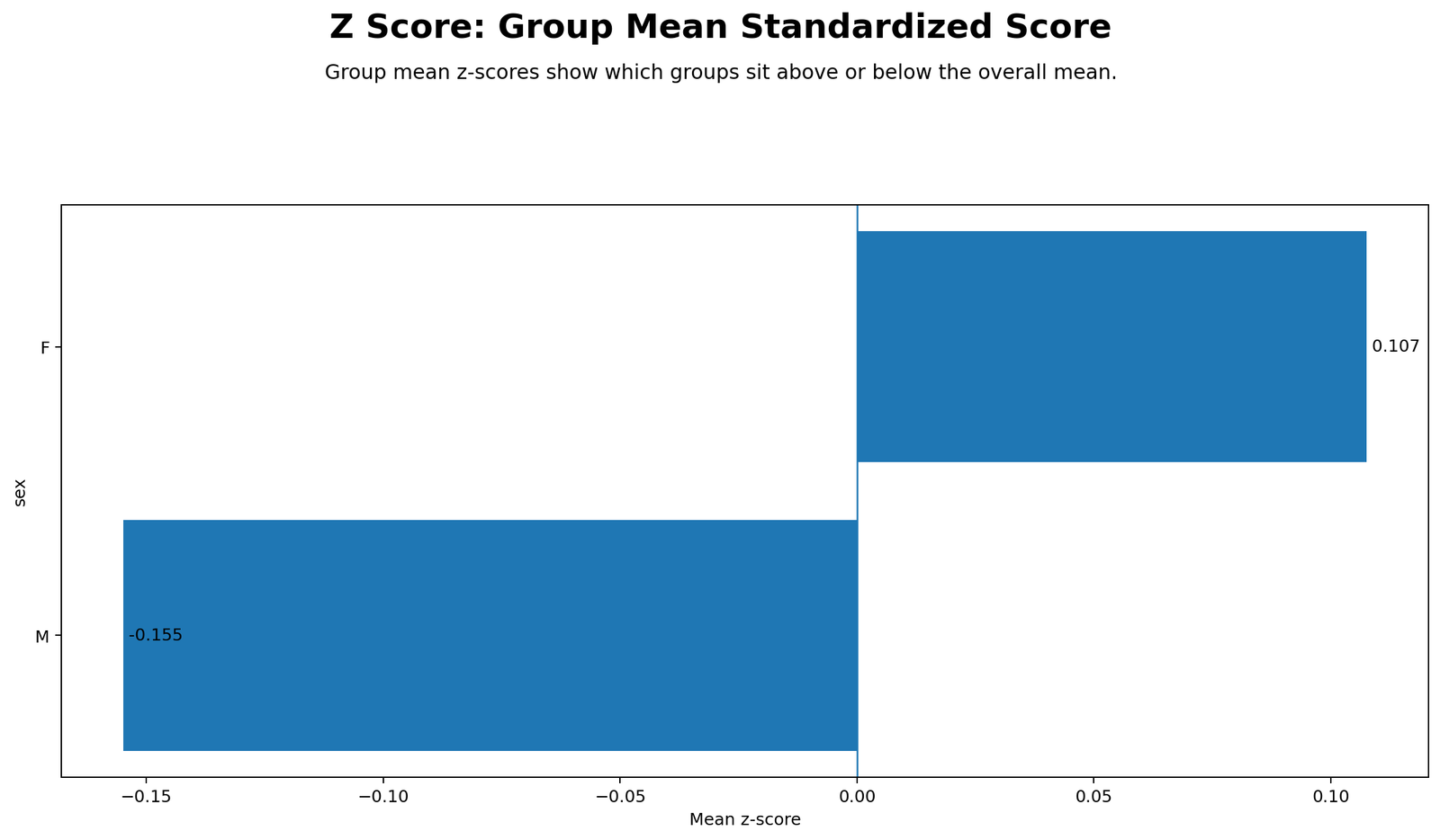
This chart compares the mean standardized G3 score by sex group. The female group has a mean Z Score of about 0.107, while the male group has a mean Z Score of about -0.155. The total standardized mean remains 0 because the full variable was standardized across all 649 cases.
This does not mean that the group difference is automatically statistically significant. It means the female group mean is slightly above the overall G3 mean, and the male group mean is slightly below it. A separate two-group mean test would be needed for a formal hypothesis decision. For descriptive interpretation, the Z Score chart gives a simple standardized effect-style view of how far each group mean sits from the overall mean.
R Chart-by-Chart Validation
The R charts validate the same Z Score results using an independent workflow. R uses the same standardization logic: subtract the mean and divide by the standard deviation. The R charts confirm that the standardized G3 distribution has mean about 0, standard deviation about 1, and a stronger lower-tail pattern than upper-tail pattern.
R Chart 1: Raw Distribution with Standard Deviation Bands
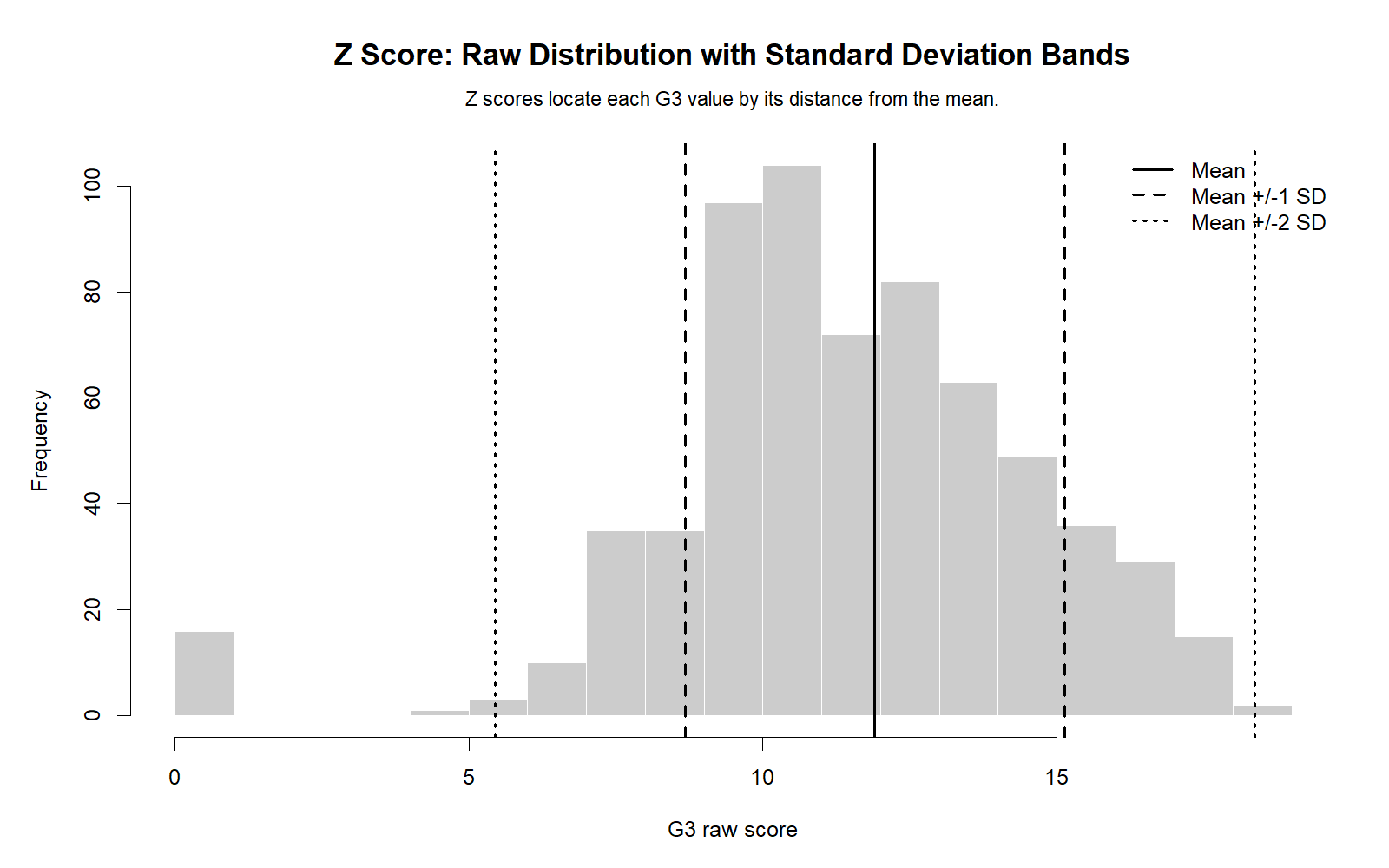
The R raw distribution chart confirms the same grade pattern shown in Python. Most G3 values are concentrated around the middle grades, while a small group of very low values sits far left of the mean. The standard deviation bands show why those values receive large negative Z Score values. The R chart therefore validates the Python interpretation that the most extreme G3 cases are low-score observations.
R Chart 2: Standardized Distribution
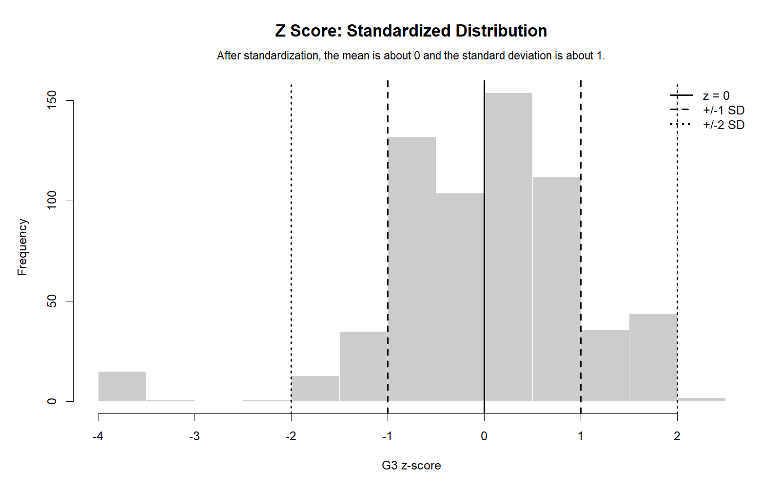
The R standardized distribution shows the same result as SPSS and Python: the mean is approximately 0, and the standard deviation is approximately 1. The left tail remains present after standardization, proving again that Z Score conversion does not make a variable normal. It only places the variable on a standard scale.
R Chart 3: Cases by Standardized Band

The R band chart confirms that most G3 cases fall between -1 and +1. It also confirms the low-tail problem: 2.5% of cases are below -3, and only 0.3% are between 2 and 3. There are no cases above +3. This pattern supports the interpretation that the extreme G3 values are concentrated on the lower side.
R Chart 4: Unusual and Extreme Values by Variable
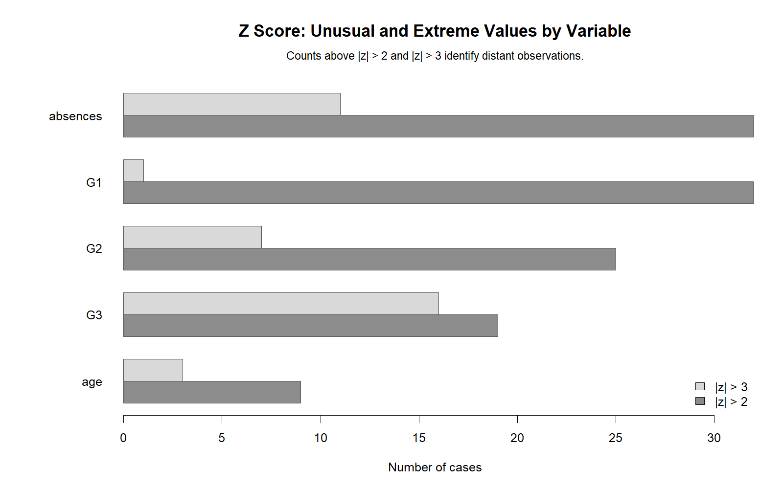
The R comparison chart confirms that the Z Score outlier pattern differs by variable. Absences has many high standardized values because some students have very high absence counts compared with the average. G1, G2, and G3 have distant low-score observations. Age has fewer unusual values, but high age values can still appear distant because age has a small standard deviation.
R Chart 5: Most Distant G3 Cases

The R most-distant-cases chart again shows that many of the farthest cases are below the mean, not above it. The standardized case list is useful for data cleaning, outlier review, and reporting. It can also be used to create a review table for the most extreme observations before deciding whether any action is needed.
R Chart 6: Group Mean Standardized Score
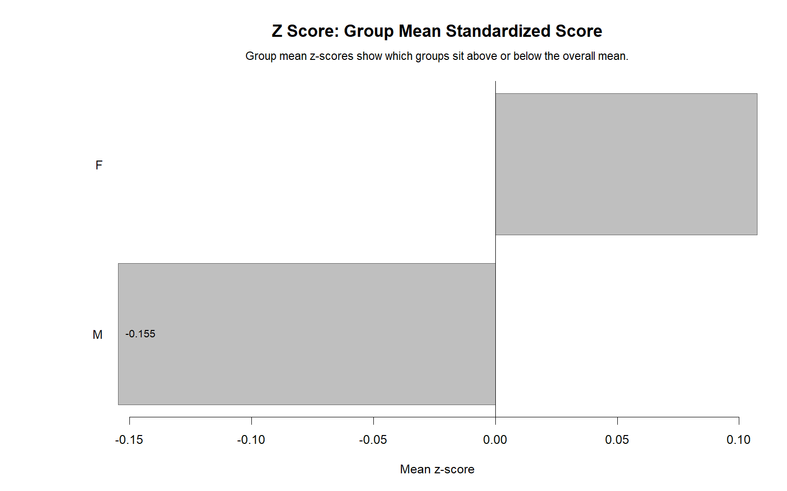
The R group chart validates the SPSS group summary. The female group sits slightly above the overall G3 mean, while the male group sits slightly below it. Because the units are standardized, the group means can be read directly as standardized distances from the overall mean. This makes the Z Score group comparison easier to interpret than raw grade differences alone.
SPSS, R, Python and Excel Workflows for Z Score
This section shows how to reproduce the Z Score analysis in SPSS, R, Python and Excel. The same logic is used in every tool: calculate the mean, calculate the standard deviation, subtract the mean from each value, and divide by the standard deviation.
SPSS Workflow
| Step | SPSS Menu or Command | Purpose |
|---|---|---|
| Import data | File > Open > Data | Load the clean SPSS-ready dataset. |
| Create Z Score variables | Analyze > Descriptive Statistics > Descriptives > Save standardized values as variables | SPSS creates z_G1, z_G2, z_G3, z_age and z_absences. |
| Check descriptive statistics | Analyze > Descriptive Statistics > Descriptives | Confirm that every standardized variable has mean 0 and standard deviation 1. |
| Create flag variables | Transform > Compute Variable | Create flags such as |z_G3| > 2 and |z_G3| > 3. |
| Create frequency tables | Analyze > Descriptive Statistics > Frequencies | Count unusual and extreme standardized cases. |
| Review plots | Analyze > Descriptive Statistics > Explore | Check histogram and boxplot for z_G3. |
| Export output | File > Export or OUTPUT EXPORT syntax | Save the SPSS output PDF for documentation and reporting. |
R Workflow
| Step | R Action | Purpose |
|---|---|---|
| Read data | read.csv() | Load the dataset into R. |
| Select variables | Create a numeric variable vector. | Keep the same variables used in SPSS and Python. |
| Standardize variables | scale() | Convert each numeric variable into a Z Score. |
| Create flags | abs(z) > 2 and abs(z) > 3 | Identify unusual and extreme standardized values. |
| Create charts | Base R or ggplot2 | Validate raw distribution, standardized distribution, bands, and group means. |
Python Workflow
| Step | Python Action | Purpose |
|---|---|---|
| Read data | pandas.read_csv() | Load the dataset into a DataFrame. |
| Convert variables | pd.to_numeric() | Prevent text or missing-value formatting from breaking the calculation. |
| Calculate Z Score | (x - mean) / sd | Create standardized variables. |
| Flag unusual values | abs(z) > 2 | Identify cases more than two standard deviations from the mean. |
| Flag extreme values | abs(z) > 3 | Identify cases more than three standard deviations from the mean. |
| Create charts | matplotlib | Generate the WordPress chart figures. |
Excel Workflow
| Excel Task | Formula Example | Purpose |
|---|---|---|
| Mean | =AVERAGE(A2:A650) | Calculate the raw mean for G3. |
| Standard deviation | =STDEV.S(A2:A650) | Calculate the sample standard deviation for G3. |
| Z Score manually | =(A2-$B$1)/$B$2 | Subtract the mean and divide by the standard deviation. |
| Z Score with STANDARDIZE | =STANDARDIZE(A2,$B$1,$B$2) | Use Excel’s built-in standardization function. |
| Absolute Z Score | =ABS(C2) | Measure distance from the mean regardless of direction. |
| Unusual flag | =IF(ABS(C2)>2,"Review","Ordinary") | Flag values beyond two standard deviations. |
| Extreme flag | =IF(ABS(C2)>3,"Extreme","Not extreme") | Flag values beyond three standard deviations. |
Code Blocks for Z Score
SPSS Syntax for Z Score
* Z Score Analysis in SPSS.
* Create standardized variables and flag unusual/extreme cases.

DATASET ACTIVATE DataSet1.

TITLE "Z Score: Standardized Scores for Key Variables".

* Create z-score variables automatically.
DESCRIPTIVES VARIABLES=G1 G2 G3 age absences
  /SAVE
  /STATISTICS=MEAN STDDEV MIN MAX.

* Rename saved standardized variables if needed.
RENAME VARIABLES (ZG1=z_G1) (ZG2=z_G2) (ZG3=z_G3) (Zage=z_age) (Zabsences=z_absences).

* Flag G3 cases beyond absolute z-score cutoffs.
COMPUTE flag_abs_z_G3_gt2 = (ABS(z_G3) > 2).
COMPUTE flag_abs_z_G3_gt3 = (ABS(z_G3) > 3).
EXECUTE.

* Create a z-score band variable for G3.
RECODE z_G3
  (Lowest thru -3 = -4)
  (-3 thru -2 = -3)
  (-2 thru -1 = -2)
  (-1 thru 0 = -1)
  (0 thru 1 = 1)
  (1 thru 2 = 2)
  (2 thru 3 = 3)
  (3 thru Highest = 4)
  INTO z_band_G3.
EXECUTE.

VARIABLE LABELS
  z_G3 "Z score for G3"
  flag_abs_z_G3_gt2 "Flag: absolute z_G3 greater than 2"
  flag_abs_z_G3_gt3 "Flag: absolute z_G3 greater than 3"
  z_band_G3 "Z-score band for G3".

FREQUENCIES VARIABLES=flag_abs_z_G3_gt2 flag_abs_z_G3_gt3 z_band_G3
  /ORDER=ANALYSIS.

EXAMINE VARIABLES=z_G3
  /PLOT=BOXPLOT HISTOGRAM
  /STATISTICS=DESCRIPTIVES
  /CINTERVAL=95
  /MISSING=LISTWISE
  /NOTOTAL.

MEANS TABLES=z_G3 BY sex
  /CELLS=COUNT MEAN STDDEV.

OUTPUT EXPORT
  /CONTENTS EXPORT=VISIBLE
  /PDF DOCUMENTFILE="Z-Score-SPSS-Output.pdf".
Python Code for Z Score
import pandas as pd
import numpy as np

df = pd.read_csv("dataset.csv")

numeric_vars = ["G1", "G2", "G3", "age", "absences"]

for col in numeric_vars:
    df[col] = pd.to_numeric(df[col], errors="coerce")
    df[f"z_{col}"] = (df[col] - df[col].mean()) / df[col].std(ddof=1)

# G3 z-score flags
df["abs_z_G3"] = df["z_G3"].abs()
df["flag_abs_z_G3_gt2"] = df["abs_z_G3"] > 2
df["flag_abs_z_G3_gt3"] = df["abs_z_G3"] > 3

summary_rows = []

for col in numeric_vars:
    z_col = f"z_{col}"
    summary_rows.append({
        "variable": col,
        "n": df[col].notna().sum(),
        "raw_mean": df[col].mean(),
        "raw_sd": df[col].std(ddof=1),
        "z_min": df[z_col].min(),
        "z_max": df[z_col].max(),
        "z_mean": df[z_col].mean(),
        "z_sd": df[z_col].std(ddof=1),
        "count_abs_z_gt_2": (df[z_col].abs() > 2).sum(),
        "count_abs_z_gt_3": (df[z_col].abs() > 3).sum()
    })

z_summary = pd.DataFrame(summary_rows)
print(z_summary)

# Band table for G3
bins = [-np.inf, -3, -2, -1, 0, 1, 2, 3, np.inf]
labels = ["below -3", "-3 to -2", "-2 to -1", "-1 to 0",
          "0 to 1", "1 to 2", "2 to 3", "above 3"]

df["z_band_G3"] = pd.cut(df["z_G3"], bins=bins, labels=labels, right=False)
band_table = df["z_band_G3"].value_counts(sort=False).to_frame("frequency")
band_table["percent"] = 100 * band_table["frequency"] / len(df)

print(band_table)

# Most distant cases
top_cases = df.assign(case_number=np.arange(1, len(df) + 1)) \
              .sort_values("abs_z_G3", ascending=False) \
              [["case_number", "G3", "z_G3", "abs_z_G3"]] \
              .head(20)

print(top_cases)
R Code for Z Score
df <- read.csv("dataset.csv")

numeric_vars <- c("G1", "G2", "G3", "age", "absences")

for (v in numeric_vars) {
  df[[v]] <- as.numeric(df[[v]])
  df[[paste0("z_", v)]] <- as.numeric(scale(df[[v]]))
}

df$abs_z_G3 <- abs(df$z_G3)
df$flag_abs_z_G3_gt2 <- df$abs_z_G3 > 2
df$flag_abs_z_G3_gt3 <- df$abs_z_G3 > 3

summary_rows <- lapply(numeric_vars, function(v) {
  zvar <- paste0("z_", v)
  data.frame(
    variable = v,
    n = sum(!is.na(df[[v]])),
    raw_mean = mean(df[[v]], na.rm = TRUE),
    raw_sd = sd(df[[v]], na.rm = TRUE),
    z_min = min(df[[zvar]], na.rm = TRUE),
    z_max = max(df[[zvar]], na.rm = TRUE),
    z_mean = mean(df[[zvar]], na.rm = TRUE),
    z_sd = sd(df[[zvar]], na.rm = TRUE),
    count_abs_z_gt_2 = sum(abs(df[[zvar]]) > 2, na.rm = TRUE),
    count_abs_z_gt_3 = sum(abs(df[[zvar]]) > 3, na.rm = TRUE)
  )
})

z_summary <- do.call(rbind, summary_rows)
print(z_summary)

df$z_band_G3 <- cut(
  df$z_G3,
  breaks = c(-Inf, -3, -2, -1, 0, 1, 2, 3, Inf),
  labels = c("below -3", "-3 to -2", "-2 to -1", "-1 to 0",
             "0 to 1", "1 to 2", "2 to 3", "above 3"),
  right = FALSE
)

band_table <- as.data.frame(table(df$z_band_G3))
band_table$percent <- 100 * band_table$Freq / nrow(df)
print(band_table)

top_cases <- df[order(-df$abs_z_G3), c("G3", "z_G3", "abs_z_G3")]
head(top_cases, 20)
Excel Formulas for Z Score
Mean:
=AVERAGE(A2:A650)

Sample standard deviation:
=STDEV.S(A2:A650)

Manual Z Score:
=(A2-$B$1)/$B$2

Excel STANDARDIZE function:
=STANDARDIZE(A2,$B$1,$B$2)

Absolute Z Score:
=ABS(C2)

Unusual value flag:
=IF(ABS(C2)>2,"Unusual / Review","Ordinary")

Extreme value flag:
=IF(ABS(C2)>3,"Extreme / Review","Not extreme")

Z Score band:
=IFS(C2<-3,"below -3",C2<-2,"-3 to -2",C2<-1,"-2 to -1",C2<0,"-1 to 0",C2<1,"0 to 1",C2<2,"1 to 2",C2<3,"2 to 3",C2>=3,"above 3")
APA Reporting Wording for Z Score
When reporting Z Score results, include the raw mean and standard deviation, confirm that the standardized variable has mean 0 and standard deviation 1, and report the number of cases exceeding the selected screening cutoffs.
APA-Style Reporting Paragraph
G3 final grade was standardized using the sample mean and sample standard deviation. The raw G3 variable had N = 649, M = 11.91, and SD = 3.231. The standardized G3 variable had M = 0.000 and SD = 1.000, confirming that the Z Score transformation was performed correctly. The minimum G3 Z Score was -3.685 and the maximum was 2.196. Using a screening rule of |z| > 2, 19 cases were flagged as unusual. Using a stricter rule of |z| > 3, 16 cases were flagged as extreme. These cases were reviewed as unusually distant observations rather than automatically removed.
Short Report Sentences
- Z Score standardization: G3 was standardized so that the transformed variable had M = 0.000 and SD = 1.000.
- Unusual values: A total of 19 G3 cases exceeded |z| > 2, indicating values more than two standard deviations from the mean.
- Extreme values: A total of 16 G3 cases exceeded |z| > 3, indicating extreme standardized values for review.
- Direction: The most distant G3 observations were below the mean, with a minimum Z Score of -3.685.
Best final wording: “The Z Score analysis showed that G3 scores were successfully standardized, with z_G3 centered at 0 and scaled to a standard deviation of 1. Most cases were ordinary, but 19 cases exceeded |z| > 2 and 16 cases exceeded |z| > 3. The most distant cases were low G3 scores, so they should be reviewed as potential extreme observations before any modeling or reporting decision.”
Common Mistakes in Z Score Interpretation
Z Score analysis is easy to calculate, but mistakes are common when interpreting the result. The main error is treating a large Z Score as automatic proof that a value is wrong. A large Z Score only tells us that the value is far from the mean.
| Mistake | Why It Is a Problem | Correct Practice |
|---|---|---|
| Deleting every case with |z| > 3 | The value may be real and meaningful. | Review the case before deleting or transforming it. |
| Thinking Z Score makes data normal | Standardization changes scale, not distribution shape. | Use normality tests and charts separately. |
| Ignoring direction | Positive and negative Z Score values have different meaning. | Report whether cases are above or below the mean. |
| Using population SD when sample SD is needed | The result can differ slightly. | Use sample standard deviation for sample data unless population parameters are known. |
| Comparing raw variables with different units | Raw scores are not always directly comparable. | Use Z Score values when variables have different scales. |
| Using Z Score for categorical variables | Categorical codes do not have meaningful standard deviation distance. | Use Z Score only for meaningful numeric variables. |
| Reporting only the maximum Z Score | The minimum may be more important. | Report both minimum and maximum Z Score values. |
When to Use Z Score
Use Z Score when you want to standardize values, compare variables with different scales, identify observations far from the mean, or create standardized scores for further analysis.
| Use Z Score When | Reason | Example from This Guide |
|---|---|---|
| You want to locate a value relative to the mean | Z Score gives distance in standard deviation units. | G3 = 19 is about 2.196 standard deviations above the mean. |
| You want to identify unusual values | |z| > 2 is a common review threshold. | 19 G3 cases exceeded |z| > 2. |
| You want to identify extreme values | |z| > 3 is a stricter review threshold. | 16 G3 cases exceeded |z| > 3. |
| You want to compare variables with different scales | Standardization places variables on the same scale. | G3, age, and absences can be compared after standardization. |
| You want to compare group means descriptively | Group mean Z Score values show standardized distance from the overall mean. | Female mean z_G3 = 0.107; male mean z_G3 = -0.155. |
| You want to prepare data for models | Standardized variables are often useful in regression, clustering, and machine learning. | z_G1, z_G2, z_G3, z_age, and z_absences can be used as standardized predictors. |
Practical rule: Use Z Score for standardized interpretation and outlier screening, but use additional statistical tests and charts before making final decisions. For normality assessment, combine Z Score review with Q-Q plots, P-P plots, Kolmogorov-Smirnov tests, and D’Agostino-Pearson tests.
Downloads and Resources for Z Score
The following resources support this Z Score guide and can be used to verify the SPSS output and reproduce the analysis.
Download SPSS Output PDF
Verified SPSS output for Z Score, including descriptive statistics, standardized variables, flag counts, band tables, plots, and group summary.
Copy Z Score Code
Use the SPSS, Python, R and Excel code blocks to reproduce the Z Score analysis.
Download note: Use the SPSS PDF as the official verification file. The Python and R charts validate the same results visually and help readers understand the standardized distribution.
FAQs About Z Score
What is a Z Score?
A Z Score is a standardized score that shows how many standard deviations a value is above or below the mean.
What is the Z Score formula?
The Z Score formula is z = (x − mean) / standard deviation. For sample data, use the sample mean and sample standard deviation.
What does a Z Score of 0 mean?
A Z Score of 0 means the raw value is exactly equal to the mean.
What does a positive Z Score mean?
A positive Z Score means the value is above the mean. For example, z = +1 means the value is one standard deviation above the mean.
What does a negative Z Score mean?
A negative Z Score means the value is below the mean. For example, z = -1 means the value is one standard deviation below the mean.
What is considered an unusual Z Score?
A common rule is that |z| > 2 indicates an unusual value that should be reviewed.
What is considered an extreme Z Score?
A common stricter rule is that |z| > 3 indicates an extreme value or possible outlier for review.
What was the Z Score result for G3 in this guide?
For G3, the standardized variable z_G3 had mean approximately 0 and standard deviation 1. The minimum z_G3 was -3.685 and the maximum z_G3 was 2.196.
How many G3 cases were unusual in this Z Score analysis?
Using |z_G3| > 2, 19 G3 cases were flagged as unusual.
How many G3 cases were extreme in this Z Score analysis?
Using |z_G3| > 3, 16 G3 cases were flagged as extreme.
Does Z Score standardization make data normal?
No. Z Score standardization changes the scale so the mean is 0 and the standard deviation is 1, but it does not remove skewness, kurtosis, or outliers.
How do I calculate Z Score in Excel?
You can calculate Z Score in Excel with =STANDARDIZE(value, mean, standard_deviation) or manually with =(value-mean)/standard_deviation.
How do I calculate Z Score in SPSS?
In SPSS, use Analyze > Descriptive Statistics > Descriptives and select “Save standardized values as variables.” SPSS will create standardized variables such as z_G3.
Should I remove cases with large Z Score values?
Not automatically. A large Z Score flags a case for review, but the analyst must check whether the value is an error, a legitimate extreme observation, or an important real case.
Can Z Score compare different variables?
Yes. Z Score standardization allows variables measured in different units to be compared on the same standard deviation scale.

