
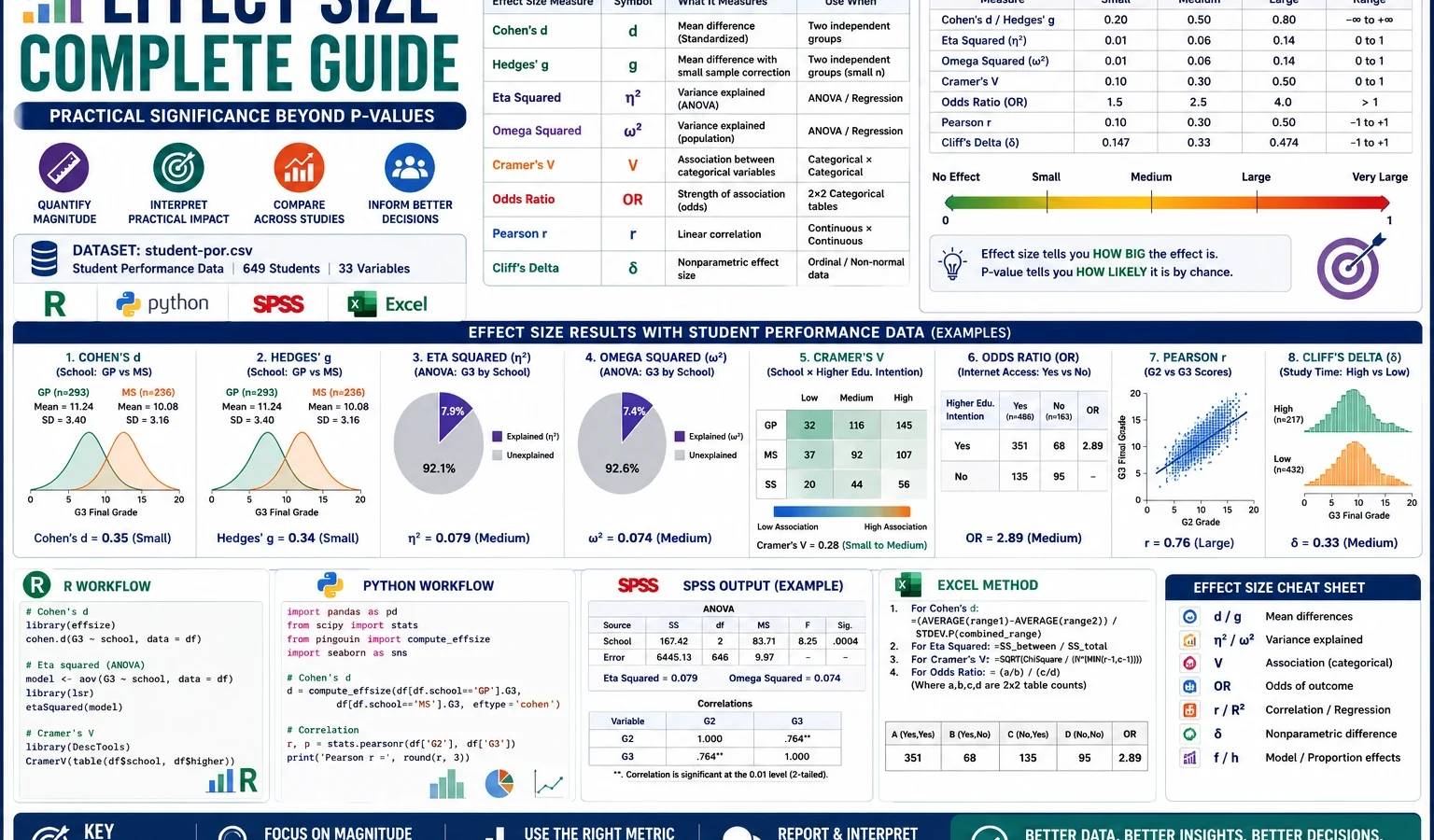
Descriptive Statistics Guide
Effect Size explains the practical size of a statistical result. A p-value can say whether a result is statistically significant, but effect size tells whether the difference, association or relationship is small, moderate, large or practically meaningful. This complete guide explains Cohen’s d, Hedges’ g, eta squared, omega squared, Cohen’s f, Cramer’s V, odds ratio, Pearson r, R squared, Cliff’s delta, R charts, Python charts, SPSS output and Excel workflow using student performance data.
Quick Answer: Effect Size Result
An Effect Size analysis was used to measure practical significance in the student performance dataset. The analysis included standardized mean differences for G3 final grade, ANOVA-style variance-explained measures, categorical association effect sizes, an odds ratio for internet access and higher education intention, a Pearson correlation between G2 and G3, and a nonparametric Cliff’s delta comparison.
Main finding: The largest practical effect is the relationship between G2 and G3, with Pearson r = .919 and R² = .844. This means second-period grade is extremely strongly related to final grade in this dataset. The strongest group mean effect is G3 by school, where Cohen’s d and Hedges’ g are both about .621, a medium-to-large practical difference.
Important interpretation note: Effect size does not replace the p-value. It adds practical meaning. A result can be statistically significant but practically small, especially in larger samples. Effect size helps explain whether the result is meaningful enough to discuss, compare or use in decision-making.
Table of Contents
- What Is Effect Size?
- Why Effect Size Is Needed with P-Values
- Effect Size Formulas and Logic
- Dataset and Variables Used
- Verified Effect Size Results
- Chart-by-Chart Interpretation
- R Code for Effect Size
- Python Code for Effect Size
- SPSS Syntax and Interpretation
- Excel Method
- Download Output and Resources
- APA Style Reporting
- When Should You Use Effect Size?
- References and Related Guides
- FAQs
What Is Effect Size?
Effect Size is a numerical measure of how large a statistical result is. It answers a different question from a p-value. A p-value asks whether the observed result is unlikely under a null hypothesis. Effect size asks how big the difference, association, relationship or explained variance is.
For example, a t test may show that two groups have significantly different G3 final grades. That is useful, but it does not fully answer the practical question: is the difference small, moderate or large? Cohen’s d answers that by standardizing the mean difference using the pooled standard deviation.
Effect size is used in education, psychology, medicine, business analytics, survey research, experimental studies and regression analysis. It is also important for meta-analysis because different studies may use different scales. Standardized effect sizes allow results from different datasets to be compared more fairly.
Simple meaning: Effect size tells the practical strength of a result. It shows how much groups differ, how strongly variables are related, how much variance a factor explains, or how strong a categorical association is.
Why Effect Size Is Needed with P-Values
A p-value is influenced by sample size. In a large dataset, a very small difference can become statistically significant. In a small dataset, a meaningful difference may fail to become statistically significant because the test has low power. This is why reporting only a p-value can be incomplete.
Effect size adds practical context. If a school difference is statistically significant but Cohen’s d is .10, the practical difference is very small. If Pearson r is .90, the relationship is very strong even before looking at a p-value. If Cramer’s V is .08, a categorical association may be statistically detectable but practically weak.
| Question | P-value answers | Effect Size answers |
|---|---|---|
| Is there evidence against the null hypothesis? | Yes or no, based on significance level. | Not the main purpose. |
| How large is the difference? | Does not directly answer. | Cohen’s d, Hedges’ g or Cliff’s delta. |
| How much variance is explained? | Does not directly answer. | Eta squared, omega squared or R squared. |
| How strong is a categorical association? | Only tests association. | Cramer’s V, odds ratio or Cohen’s h. |
| How strong is a numeric relationship? | Can test correlation significance. | Pearson r and R squared show strength. |
Effect Size Formulas and Logic
Different research questions need different effect size formulas. The correct effect size depends on whether the variables are numeric, categorical, grouped, paired, independent, parametric or nonparametric.
Cohen's d:
d = (Mean1 - Mean2) / pooled standard deviation

Hedges' g:
g = J × d
where J is a small-sample correction factor

Eta squared:
η² = SS_between / SS_total

Omega squared:
ω² = (SS_between - df_between × MS_within) / (SS_total + MS_within)

Cohen's f:
f = sqrt(η² / (1 - η²))

Cramer's V:
V = sqrt(χ² / (n × min(r - 1, c - 1)))

Odds ratio:
OR = (a × d) / (b × c)

Pearson r:
r = covariance(x, y) / (standard deviation of x × standard deviation of y)

R squared:
R² = r² for simple linear correlation

Cliff's delta:
δ = P(X > Y) - P(X < Y)| Effect size method | Best used for | Typical interpretation guide |
|---|---|---|
| Cohen’s d | Mean difference between two groups | .20 small, .50 medium, .80 large |
| Hedges’ g | Mean difference with sample-size correction | Similar to Cohen’s d |
| Eta squared | ANOVA variance explained | .01 small, .06 medium, .14 large |
| Omega squared | Less biased ANOVA variance explained | Usually slightly smaller than eta squared |
| Cramer’s V | Categorical association | Roughly .10 small, .30 medium, .50 large |
| Odds ratio | 2 × 2 categorical comparison | 1 means no odds difference; above 1 means higher odds |
| Pearson r | Linear association between two numeric variables | .10 small, .30 medium, .50 large |
| Cliff’s delta | Nonparametric two-group difference | About .147 small, .33 medium, .474 large |
Cutoff warning: Interpretation cutoffs are only general rules. A small effect can be important in clinical, policy or high-volume business settings. A large effect can be less useful if it comes from poor measurement or a biased design.
Dataset and Variables Used
This guide uses the student-por.csv student performance dataset with 649 rows. The main numeric outcome is G3, which represents final grade. The analysis also uses G2 for correlation, plus categorical grouping variables such as school, sex, internet access, romantic relationship, study time, failure group, school support and higher education intention.
| Item | Variable | Role in this effect size guide |
|---|---|---|
| Final grade | G3 | Main numeric outcome for group differences and ANOVA effect sizes. |
| Second-period grade | G2 | Used with G3 to calculate Pearson r and R squared. |
| School group | school | Used for Cohen’s d, Hedges’ g, eta squared, omega squared and Cliff’s delta. |
| Sex | sex | Used for standardized G3 mean difference. |
| Internet access | internet | Used for G3 mean difference and odds ratio with higher education intention. |
| Higher education intention | higher | Used as a categorical outcome for Cramer’s V, odds ratio and Cohen’s h. |
| Study time | studytime | Used for ANOVA-style variance explained in G3. |
| Failure group | failure_group | Used for eta squared, omega squared and Cohen’s f. |
External dataset source: UCI Machine Learning Repository: Student Performance dataset.
Verified Effect Size Results
The R, Python and SPSS outputs agree on the main practical-significance pattern. Pearson r between G2 and G3 is the dominant effect. School differences in G3 are also practically meaningful. Most Cramer’s V values are very small to small, which means the categorical associations are present but not strong in practical terms.
| Effect size method | Comparison | Verified value | Practical interpretation |
|---|---|---|---|
| Cohen’s d | G3 by school | .621 | Medium to large standardized mean difference. |
| Cohen’s d | G3 by sex | .264 | Small to medium difference. |
| Cohen’s d | G3 by romantic relationship | .188 | Small difference. |
| Cohen’s d | G3 by internet access | -.359 | Small to medium negative direction depending on group ordering. |
| Hedges’ g | G3 by school | .621 | Small-sample corrected value remains medium to large. |
| Eta squared | G3 by failure group | .193 | Largest ANOVA-style variance-explained effect. |
| Omega squared | G3 by failure group | .189 | Adjusted variance-explained estimate remains strong. |
| Cramer’s V | School by higher education intention | .136 | Small categorical association. |
| Odds ratio | Internet access by higher education intention | 1.65 | Higher odds of higher-education intention for the selected group, but confidence interval should be checked. |
| Pearson r | G2 by G3 | .919 | Very strong positive linear association. |
| R squared | G2 predicting G3 | .844 | About 84.4% of G3 variation is explained by G2 in a simple linear relationship. |
| Cliff’s delta | G3 by school | .344 | Small to medium nonparametric difference. |
The SPSS output also reports 649 valid cases for the main variables, G3 mean = 11.9060, G3 standard deviation = 3.23066, GP mean G3 = 12.5768 and MS mean G3 = 10.6504. These raw means explain why the school effect size is one of the largest group-difference effects in this worked example.
Chart-by-Chart Interpretation of the Effect Size Analysis
This section explains the uploaded R and Python charts. Python charts use a clean title and subtitle layout for better readability, while R charts confirm the same analytical pattern in a second software workflow.
Chart 1: Cohen’s d for G3 Group Differences
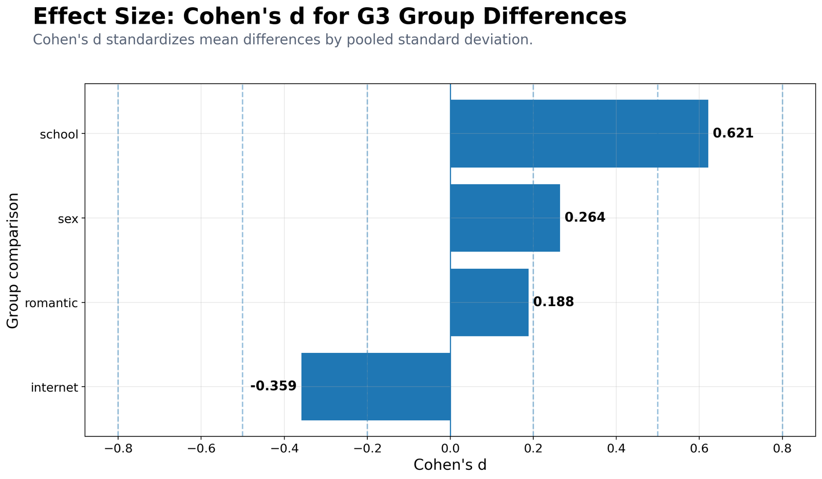
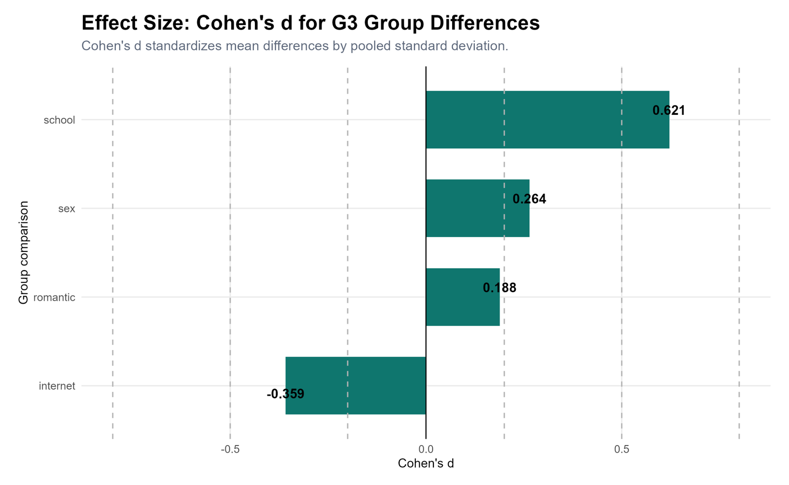
Specific interpretation: Cohen’s d is largest for G3 by school at .621. This is a medium-to-large practical difference, meaning the average final grade difference between school groups is meaningful after standardization. The sex effect is .264, which is small to medium. Romantic relationship has a small effect at .188. Internet access has a negative value, -.359, because the sign depends on group order; the absolute size is small to medium.
Decision from Chart 1: School group is the strongest standardized two-group mean difference for G3 among the comparisons shown.
Chart 2: Hedges’ g with Small-Sample Correction
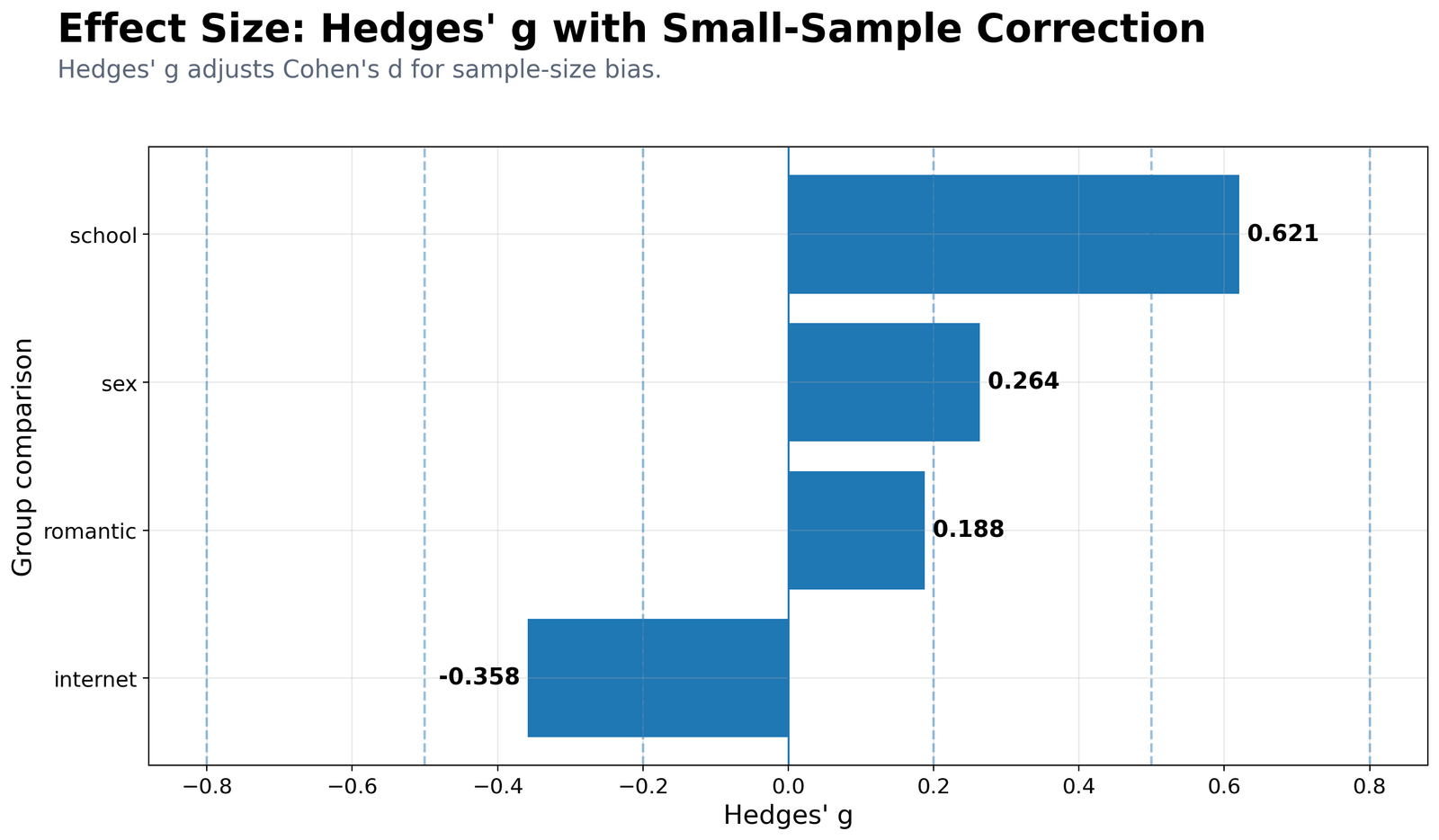
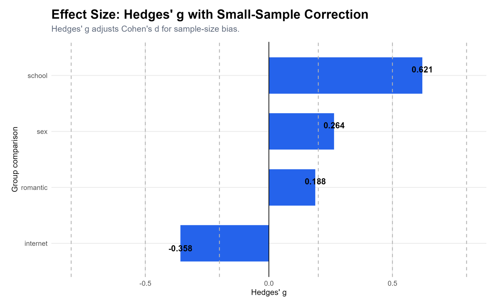
Specific interpretation: Hedges’ g corrects Cohen’s d for small-sample bias. In this dataset, the values are almost the same as Cohen’s d because the sample size is large. School remains .621, sex remains .264, romantic relationship remains .188, and internet access is -.358.
Decision from Chart 2: The small-sample correction does not change the practical conclusion. School remains the most important two-group G3 difference.
Chart 3: Eta Squared and Omega Squared
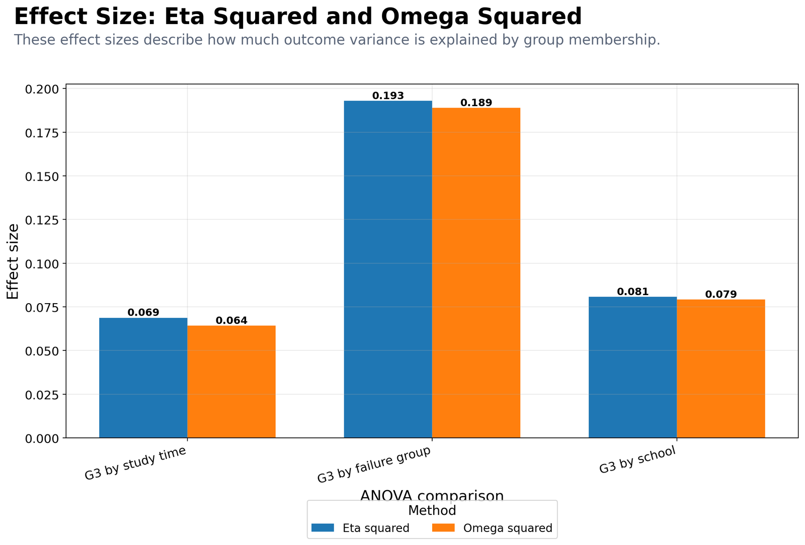
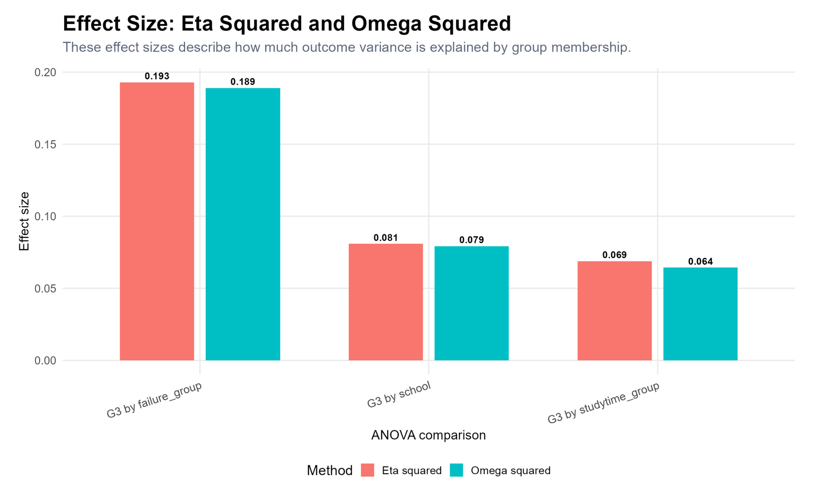
Specific interpretation: The strongest variance-explained effect is G3 by failure group, with eta squared = .193 and omega squared = .189. This means failure-history grouping explains a meaningful share of final grade variation. G3 by school has eta squared = .081 and omega squared = .079. G3 by study time has eta squared = .069 and omega squared = .064.
Decision from Chart 3: Failure group explains the largest share of G3 variation among the ANOVA-style comparisons.
Chart 4: Cramer’s V for Categorical Associations
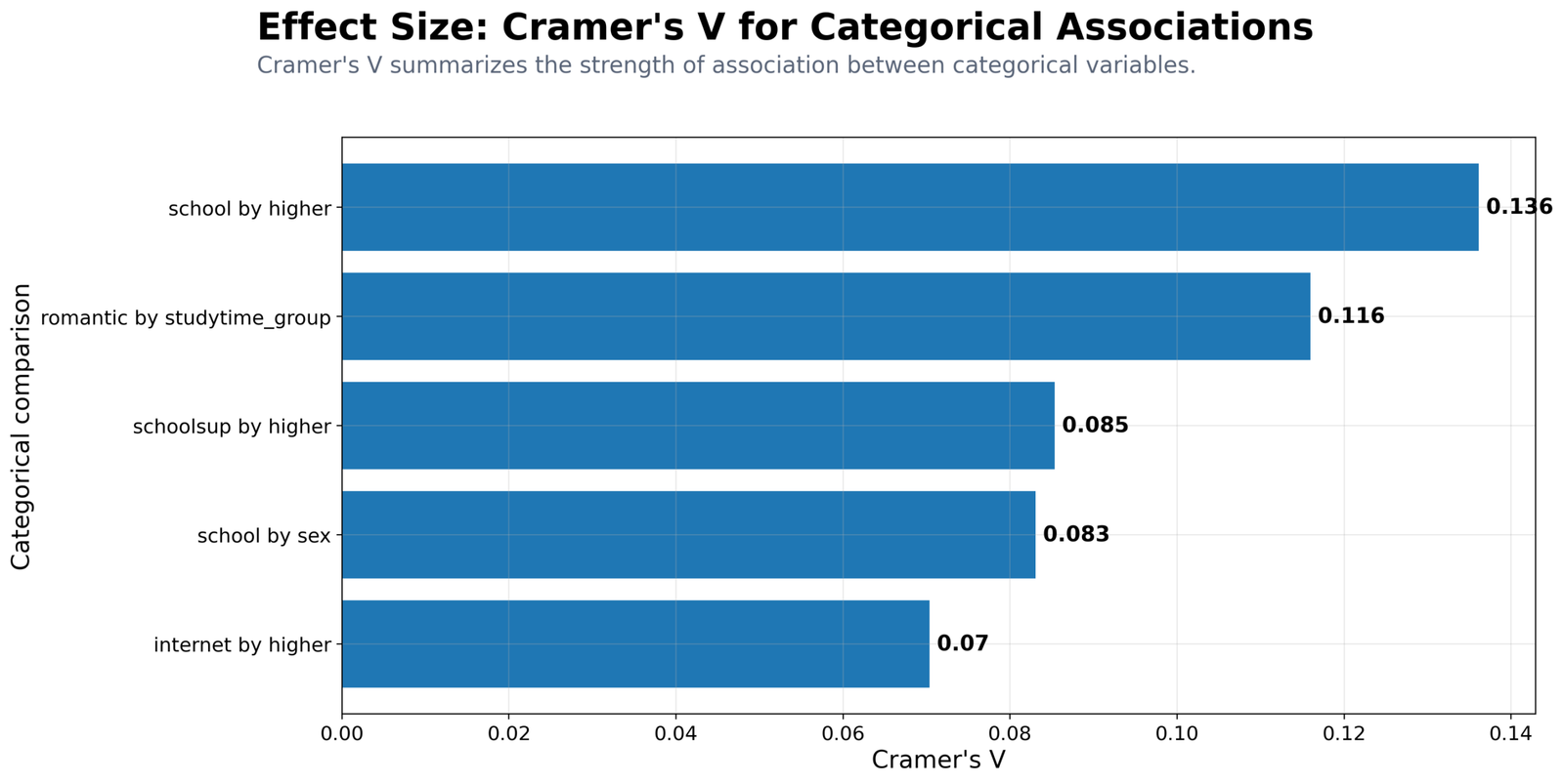
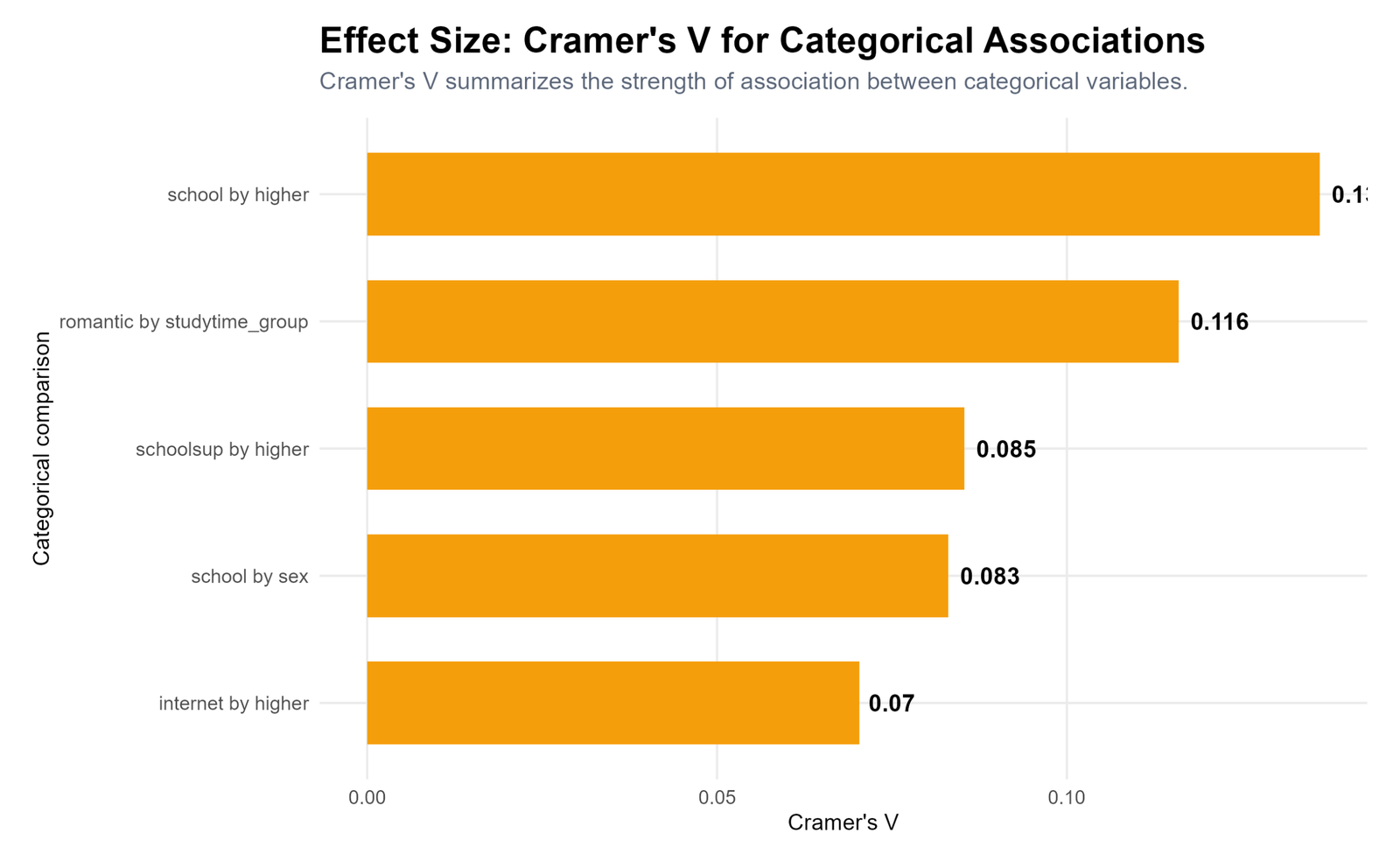
Specific interpretation: The largest categorical association shown is school by higher education intention with Cramer’s V = .136. Romantic relationship by study-time group has V = .116. School support by higher has V = .085, school by sex has V = .083, and internet by higher has V = .070. These are very small to small practical associations.
Decision from Chart 4: Categorical associations exist, but their practical strength is much weaker than the G2-G3 numeric relationship.
Chart 5: Odds Ratio for Internet Access and Higher Education Intention
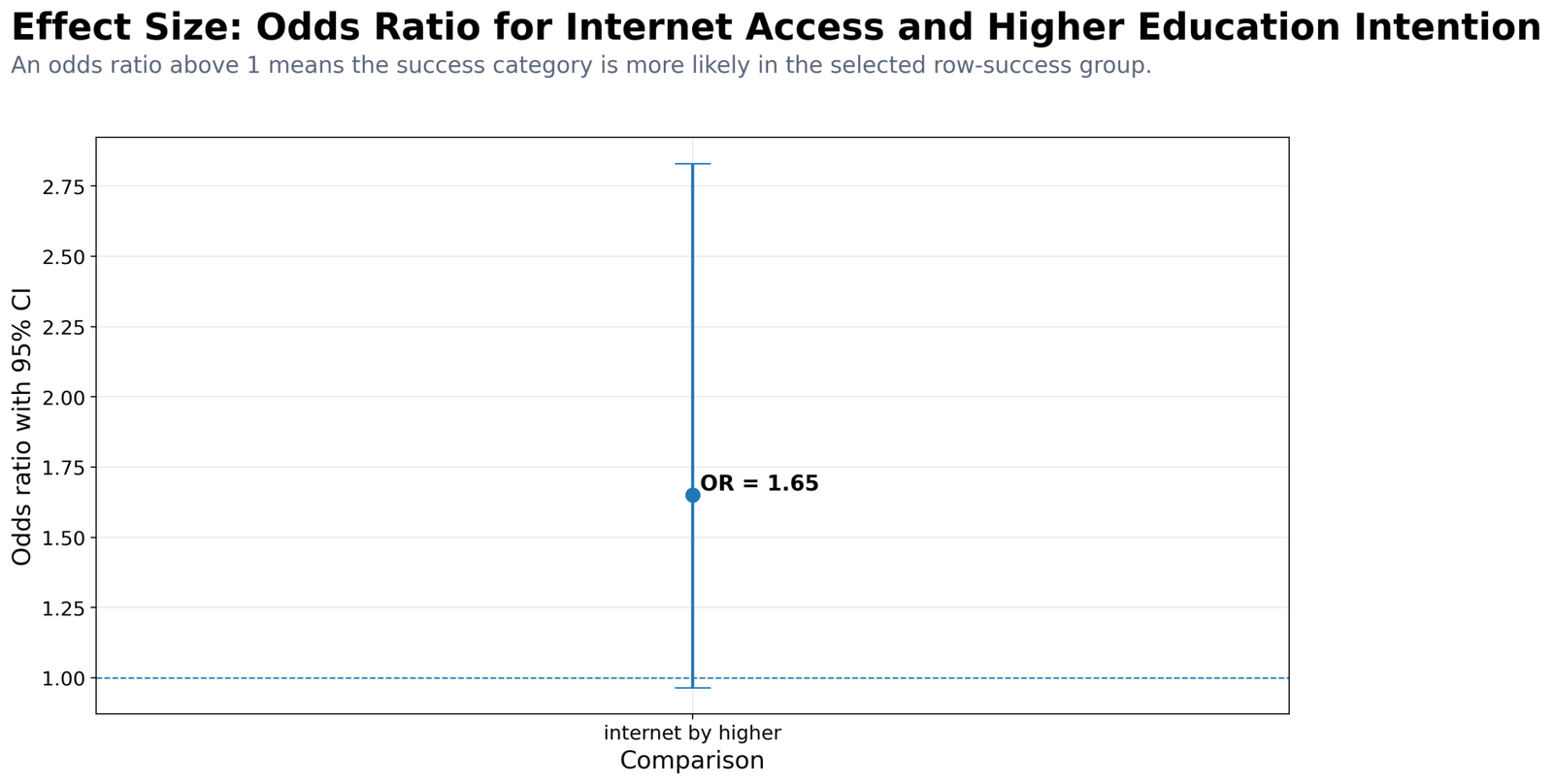
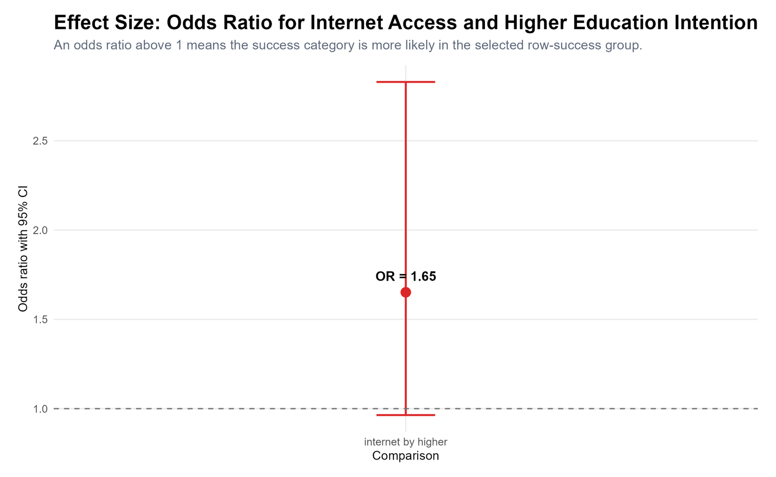
Specific interpretation: The odds ratio is 1.65. An odds ratio above 1 means the success category is more likely in the selected row-success group. Here, internet access is associated with higher odds of intending higher education. However, the confidence interval reaches close to 1, so the result should be interpreted cautiously rather than overstated.
Decision from Chart 5: Internet access shows a positive odds-ratio direction for higher education intention, but the practical strength is small.
Chart 6: Pearson r Between G2 and G3
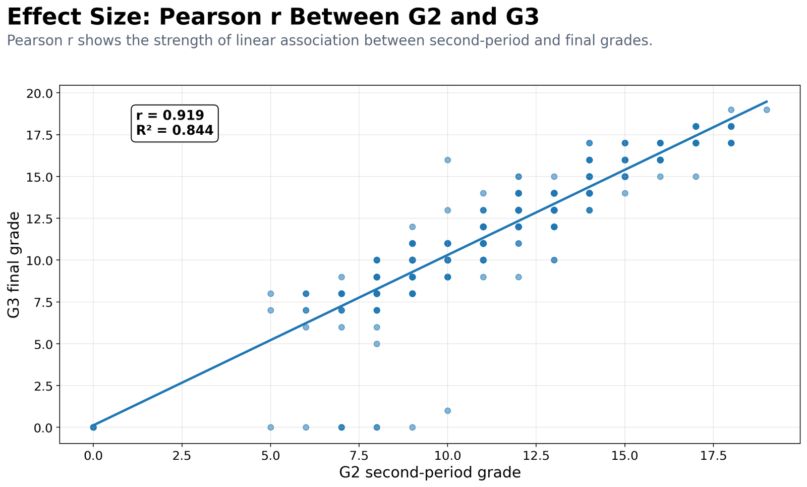
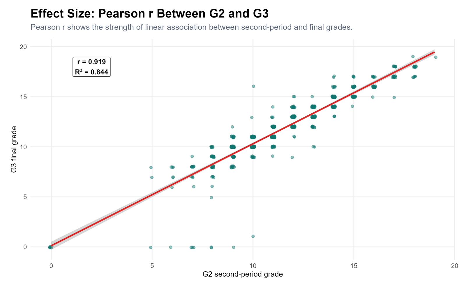
Specific interpretation: Pearson r is .919, which is a very strong positive relationship. The fitted line rises sharply because students with higher G2 grades usually have higher G3 grades. R squared is .844, meaning about 84.4% of the variation in G3 is explained by G2 in a simple relationship.
Decision from Chart 6: G2 is the strongest practical predictor or companion variable for G3 in this effect size analysis.
Chart 7: Effect Size Summary Panel
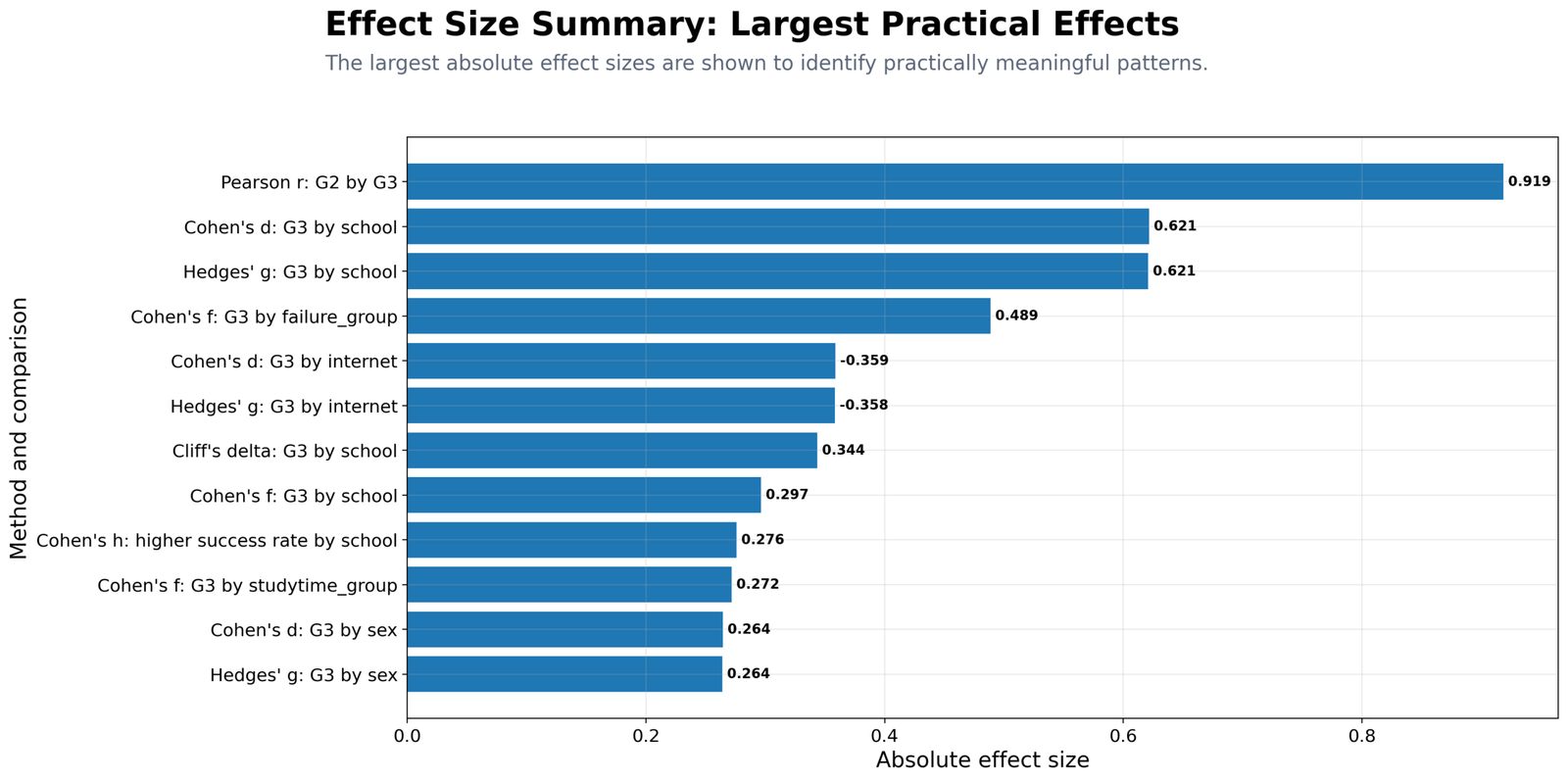
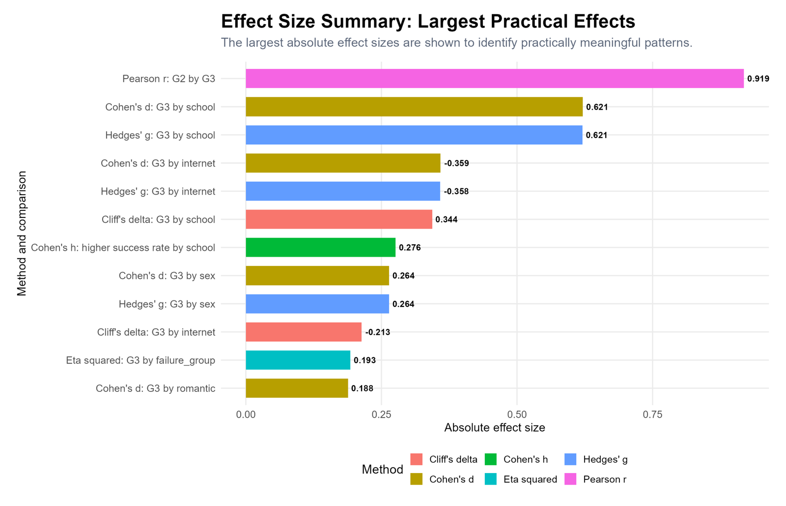
Specific interpretation: The summary panel makes the practical hierarchy clear. Pearson r for G2 by G3 is highest at .919. Cohen’s d and Hedges’ g for G3 by school follow at .621. Cohen’s f for G3 by failure group is .489. The internet G3 difference appears with an absolute effect around .359. These results help identify the effects worth discussing first.
Decision from Chart 7: The most practically meaningful story is not every significant result. The main story is the very strong G2-G3 relationship and the meaningful school and failure-group effects on G3.
Chart 8: Raw Mean Difference Context for G3
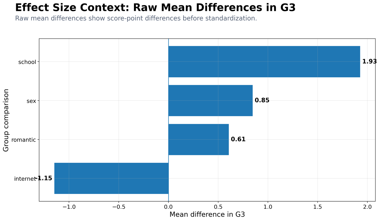
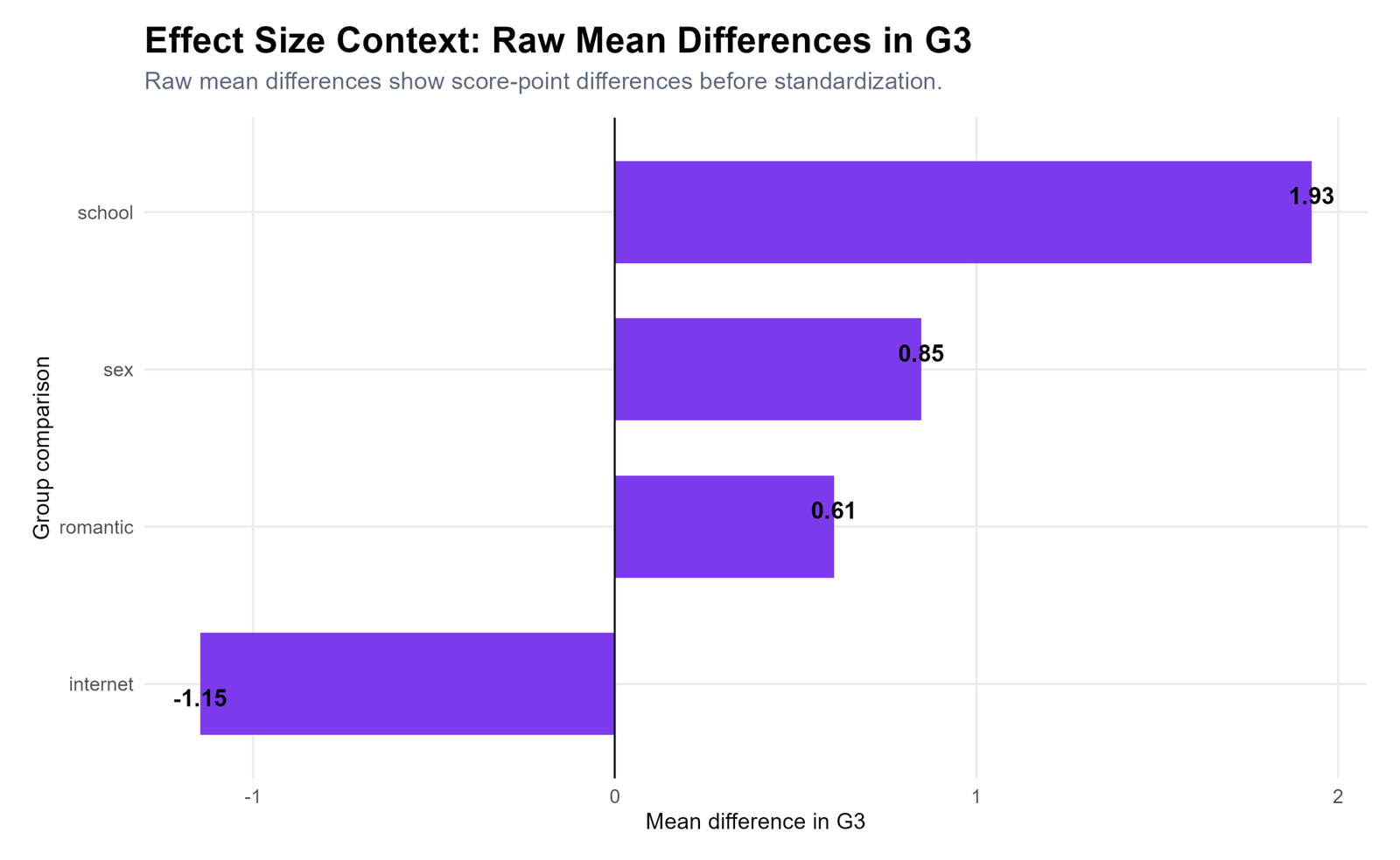
Specific interpretation: Raw mean differences explain the real score-point gap behind standardized effect sizes. The school comparison shows about 1.93 G3 points difference. Sex shows about .85 points. Romantic relationship shows about .61 points. Internet access shows about -1.15 points depending on the group order used in the calculation.
Decision from Chart 8: Standardized effect sizes are easier to compare, but raw mean differences are easier for readers to understand in the original grade scale.
Chart 9: Cliff’s Delta for Nonparametric Group Difference
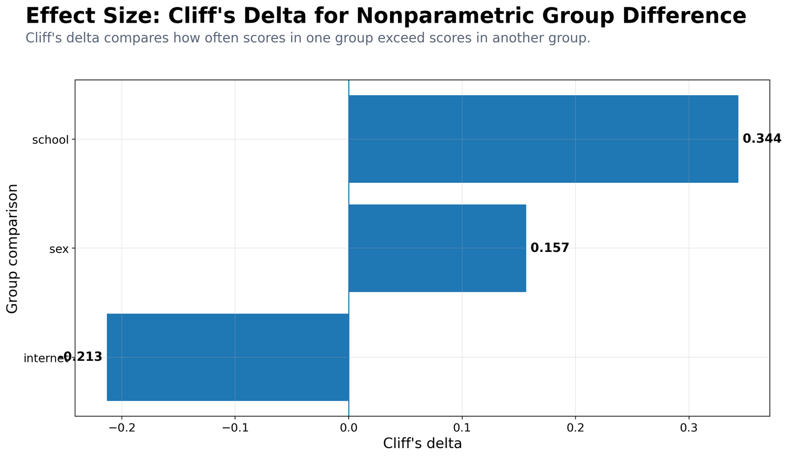
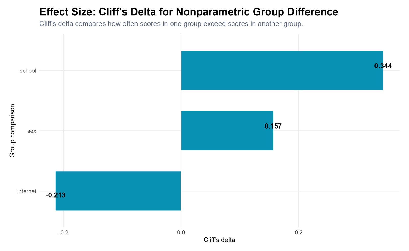
Specific interpretation: Cliff’s delta compares how often scores in one group exceed scores in another group. School has Cliff’s delta = .344, a small-to-medium nonparametric effect. Sex has .157, a small effect. Internet access has -.213, a small-to-medium negative direction depending on group order.
Decision from Chart 9: The nonparametric effect size supports the same conclusion as Cohen’s d: school is the strongest two-group difference for G3.
Chart 10: Practical Significance Interpretation
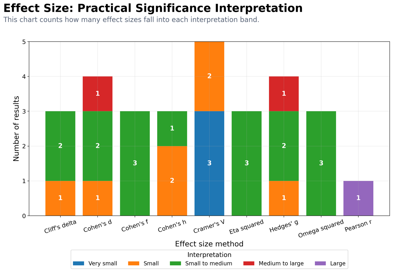
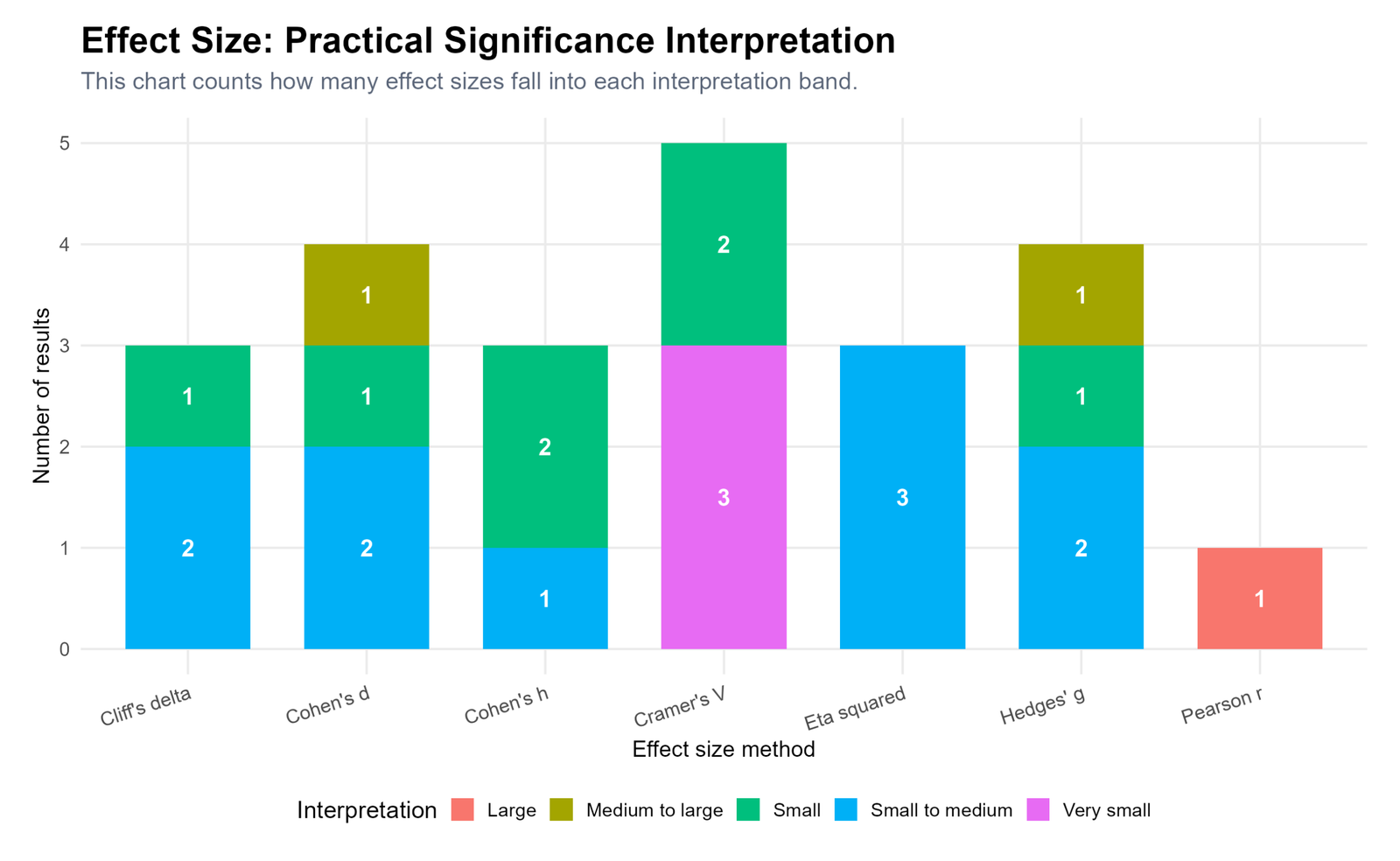
Specific interpretation: This chart groups effect sizes into practical interpretation bands. It shows that the analysis includes very small, small, small-to-medium, medium-to-large and large effects. Pearson r provides the large effect. Cohen’s d, Hedges’ g, Cohen’s f and Cliff’s delta provide several small-to-medium or medium-to-large patterns. Cramer’s V values are mostly very small or small.
Decision from Chart 10: The dataset contains a mix of practical effect sizes, but the largest effects are concentrated around grade continuity and school/failure-group differences.
R Code for Effect Size
R can calculate effect sizes using direct formulas and packages. The simplified workflow below shows how to calculate Cohen’s d, Hedges’ g, eta squared, omega squared, Cramer’s V, odds ratio and Pearson r.
library(readr)
library(dplyr)
library(effectsize)
library(rcompanion)

folder <- "D:/DATA ANALYSIS/A Basic Descriptive Statistics Guides/Effect Size"
data_file <- file.path(folder, "clean data set.csv")

df <- read_csv(data_file, show_col_types = FALSE) %>%
  mutate(
    sex = factor(sex, levels = c("F", "M"), labels = c("Female", "Male")),
    higher = factor(higher, levels = c("no", "yes"), labels = c("No", "Yes")),
    internet = factor(internet, levels = c("no", "yes"), labels = c("No", "Yes")),
    romantic = factor(romantic, levels = c("no", "yes"), labels = c("No", "Yes"))
  )

# Cohen's d and Hedges' g for G3 by school
cohens_d(G3 ~ school, data = df)
hedges_g(G3 ~ school, data = df)

# Eta squared and omega squared
model_school <- aov(G3 ~ school, data = df)
eta_squared(model_school)
omega_squared(model_school)

# Cramer's V for school by higher education intention
ct_school_higher <- table(df$school, df$higher)
cramerV(ct_school_higher)

# Odds ratio for internet by higher education intention
ct_internet_higher <- table(df$internet, df$higher)
oddsratio(ct_internet_higher)

# Pearson r and R squared
cor_value <- cor(df$G2, df$G3, use = "complete.obs")
r_squared <- cor_value^2
cor_value
r_squared
R interpretation: R confirms the main practical-significance pattern. The school difference in G3 is meaningful, failure group explains the largest ANOVA-style share of G3 variance, and G2 has a very strong correlation with G3.
Python Code for Effect Size
Python is useful for automatic effect size reporting because it can calculate values, save clean SPSS-ready data, create charts and export summary tables in one workflow.
import numpy as np
import pandas as pd
from scipy import stats
from scipy.stats import chi2_contingency

folder = r"D:\DATA ANALYSIS\A Basic Descriptive Statistics Guides\Effect Size"
data_file = folder + r"\clean data set.csv"

df = pd.read_csv(data_file)
df["sex"] = df["sex"].map({"F": "Female", "M": "Male"})
df["higher"] = df["higher"].map({"no": "No", "yes": "Yes"})
df["internet"] = df["internet"].map({"no": "No", "yes": "Yes"})
df["romantic"] = df["romantic"].map({"no": "No", "yes": "Yes"})

def cohens_d(x, y):
    x = pd.Series(x).dropna()
    y = pd.Series(y).dropna()
    nx, ny = len(x), len(y)
    pooled_sd = np.sqrt(((nx - 1) * x.var(ddof=1) + (ny - 1) * y.var(ddof=1)) / (nx + ny - 2))
    return (x.mean() - y.mean()) / pooled_sd

def hedges_g_from_d(d, n1, n2):
    dfree = n1 + n2 - 2
    correction = 1 - (3 / (4 * dfree - 1))
    return d * correction

def cramers_v(table):
    chi2, p, dof, expected = chi2_contingency(table, correction=False)
    n = table.to_numpy().sum()
    r, k = table.shape
    return np.sqrt(chi2 / (n * min(r - 1, k - 1)))

# Cohen's d for G3 by school
gp = df.loc[df["school"] == "GP", "G3"]
ms = df.loc[df["school"] == "MS", "G3"]
d_school = cohens_d(gp, ms)
g_school = hedges_g_from_d(d_school, len(gp), len(ms))

# Pearson r and R squared
r_value, p_value = stats.pearsonr(df["G2"], df["G3"])
r_squared = r_value ** 2

# Cramer's V example
ct = pd.crosstab(df["school"], df["higher"])
v = cramers_v(ct)

print("Cohen's d, G3 by school:", round(d_school, 3))
print("Hedges' g, G3 by school:", round(g_school, 3))
print("Pearson r, G2 by G3:", round(r_value, 3))
print("R squared:", round(r_squared, 3))
print("Cramer's V, school by higher:", round(v, 3))
Python chart title note: For all future charts, keep the title and subtitle separated using fig.suptitle(), fig.text() and fig.subplots_adjust(top=...). This prevents title overlap and keeps the final WordPress images readable.
SPSS Syntax and Interpretation for Effect Size
SPSS can calculate several effect size measures directly or indirectly. Independent-samples t tests can display effect sizes in newer SPSS versions. ONEWAY and GLM can support ANOVA-style effect interpretation. Crosstabs provide Phi and Cramer’s V for categorical association. Correlations provide Pearson r.
The uploaded SPSS output file is available below:
View Effect Size SPSS Output PDF
SPSS Menu Method
| Effect size need | SPSS menu path | Output to read |
|---|---|---|
| Cohen’s d or Hedges’ g context | Analyze → Compare Means → Independent-Samples T Test | Group means, mean difference and effect size table if available. |
| Eta squared or omega squared context | Analyze → Compare Means → One-Way ANOVA | ANOVA table, between-groups sum of squares and total sum of squares. |
| Cramer’s V | Analyze → Descriptive Statistics → Crosstabs | Symmetric Measures table. |
| Odds ratio | Analyze → Descriptive Statistics → Crosstabs → Statistics → Risk | Risk Estimate table for a 2 × 2 table. |
| Pearson r | Analyze → Correlate → Bivariate | Pearson correlation coefficient and significance value. |
SPSS Syntax Example with PDF Export
SET PRINTBACK=ON MPRINT=ON DECIMAL=DOT.
SET UNICODE=ON.

HOST COMMAND=['cmd /c if not exist "D:\DATA ANALYSIS\A Basic Descriptive Statistics Guides\Effect Size\Python_Output\pdf" mkdir "D:\DATA ANALYSIS\A Basic Descriptive Statistics Guides\Effect Size\Python_Output\pdf"'].

GET DATA
 /TYPE=TXT
 /FILE='D:\DATA ANALYSIS\A Basic Descriptive Statistics Guides\Effect Size\Python_Output\clean_data\effect_size_clean_data_for_spss.csv'
 /ENCODING='UTF8'
 /DELCASE=LINE
 /DELIMITERS=","
 /QUALIFIER='"'
 /ARRANGEMENT=DELIMITED
 /FIRSTCASE=2
 /VARIABLES=
 school A8
 sex A12
 age F8.2
 studytime F8.2
 failures F8.2
 schoolsup A8
 higher A8
 internet A8
 romantic A8
 absences F8.2
 G1 F8.2
 G2 F8.2
 G3 F8.2
 studytime_group A20
 failure_group A20.
CACHE.
EXECUTE.

DATASET NAME EffectSizeMain WINDOW=FRONT.

NUMERIC school_num sex_num internet_num higher_num schoolsup_num romantic_num (F1.0).
DO IF (school = "GP").
 COMPUTE school_num = 1.
ELSE IF (school = "MS").
 COMPUTE school_num = 2.
END IF.
DO IF (sex = "Female").
 COMPUTE sex_num = 1.
ELSE IF (sex = "Male").
 COMPUTE sex_num = 2.
END IF.
DO IF (internet = "No").
 COMPUTE internet_num = 0.
ELSE IF (internet = "Yes").
 COMPUTE internet_num = 1.
END IF.
DO IF (higher = "No").
 COMPUTE higher_num = 0.
ELSE IF (higher = "Yes").
 COMPUTE higher_num = 1.
END IF.
DO IF (schoolsup = "No").
 COMPUTE schoolsup_num = 0.
ELSE IF (schoolsup = "Yes").
 COMPUTE schoolsup_num = 1.
END IF.
DO IF (romantic = "No").
 COMPUTE romantic_num = 0.
ELSE IF (romantic = "Yes").
 COMPUTE romantic_num = 1.
END IF.
EXECUTE.

VARIABLE LABELS
 school_num "School group"
 sex_num "Sex"
 internet_num "Internet access"
 higher_num "Higher education intention"
 schoolsup_num "School support"
 romantic_num "Romantic relationship"
 G1 "First period grade"
 G2 "Second period grade"
 G3 "Final grade".

VALUE LABELS school_num 1 "GP" 2 "MS".
VALUE LABELS sex_num 1 "Female" 2 "Male".
VALUE LABELS internet_num 0 "No" 1 "Yes".
VALUE LABELS higher_num 0 "No" 1 "Yes".
VALUE LABELS schoolsup_num 0 "No" 1 "Yes".
VALUE LABELS romantic_num 0 "No" 1 "Yes".
VALUE LABELS studytime 1 "<2 hours" 2 "2 to 5 hours" 3 "5 to 10 hours" 4 ">10 hours".
VALUE LABELS failures 0 "0 failures" 1 "1 failure" 2 "2 failures" 3 "3+ failures".
EXECUTE.

TITLE "Effect Size Analysis".
SUBTITLE "Practical significance results".

DESCRIPTIVES VARIABLES=G1 G2 G3 age absences studytime failures
 /STATISTICS=MEAN STDDEV MIN MAX.

MEANS TABLES=G3 BY school_num sex_num internet_num romantic_num
 /CELLS=COUNT MEAN STDDEV MEDIAN MIN MAX.

T-TEST GROUPS=school_num(1 2)
 /MISSING=ANALYSIS
 /VARIABLES=G3
 /CRITERIA=CI(.95)
 /ES DISPLAY(TRUE).

T-TEST GROUPS=sex_num(1 2)
 /MISSING=ANALYSIS
 /VARIABLES=G3
 /CRITERIA=CI(.95)
 /ES DISPLAY(TRUE).

T-TEST GROUPS=internet_num(0 1)
 /MISSING=ANALYSIS
 /VARIABLES=G3
 /CRITERIA=CI(.95)
 /ES DISPLAY(TRUE).

ONEWAY G3 BY school_num
 /STATISTICS DESCRIPTIVES HOMOGENEITY EFFECTS
 /MISSING ANALYSIS.

ONEWAY G3 BY studytime
 /STATISTICS DESCRIPTIVES HOMOGENEITY EFFECTS
 /MISSING ANALYSIS.

CROSSTABS
 /TABLES=school_num BY higher_num
 /STATISTICS=CHISQ PHI
 /CELLS=COUNT ROW COLUMN EXPECTED.

CROSSTABS
 /TABLES=internet_num BY higher_num
 /STATISTICS=CHISQ RISK PHI
 /CELLS=COUNT ROW COLUMN EXPECTED.

CORRELATIONS
 /VARIABLES=G2 G3
 /PRINT=TWOTAIL NOSIG
 /MISSING=PAIRWISE.

OUTPUT SAVE
 OUTFILE='D:\DATA ANALYSIS\A Basic Descriptive Statistics Guides\Effect Size\Python_Output\pdf\Effect-Size-SPSS-Output.spv'
 LOCK=NO.

OUTPUT EXPORT
 /CONTENTS EXPORT=ALL LAYERS=PRINTSETTING MODELVIEWS=PRINTSETTING
 /PDF DOCUMENTFILE='D:\DATA ANALYSIS\A Basic Descriptive Statistics Guides\Effect Size\Python_Output\pdf\Effect-Size-SPSS-Output.pdf'
 /EMBEDBOOKMARKS=YES
 /EMBEDFONTS=YES.
Excel Method for Effect Size
Excel can calculate several effect sizes manually. It is not as automatic as R, Python or SPSS, but it is useful for teaching formulas and checking smaller examples.
Excel Steps for Cohen’s d
| Step | Excel action | Formula idea |
|---|---|---|
| 1 | Filter G3 by two groups, such as GP and MS. | Create two columns of G3 scores. |
| 2 | Calculate each group mean. | =AVERAGE(range) |
| 3 | Calculate each group standard deviation. | =STDEV.S(range) |
| 4 | Calculate group sample sizes. | =COUNT(range) |
| 5 | Calculate pooled standard deviation. | =SQRT(((n1-1)*sd1^2+(n2-1)*sd2^2)/(n1+n2-2)) |
| 6 | Calculate Cohen’s d. | =(mean1-mean2)/pooled_sd |
Excel Steps for Pearson r and R Squared
| Output | Excel formula | Interpretation |
|---|---|---|
| Pearson r | =CORREL(G2_range,G3_range) | Strength and direction of linear association. |
| R squared | =CORREL(G2_range,G3_range)^2 | Proportion of variation explained in a simple linear relationship. |
| Odds ratio | =(a*d)/(b*c) | Odds comparison for a 2 × 2 table. |
| Eta squared | =SS_between/SS_total | ANOVA variance explained. |
Download Output and Resources
The SPSS PDF output and dataset source are available below. Use the SPSS output for formal tables and use the R/Python charts for visual interpretation of practical significance.
APA Style Reporting for Effect Size
An effect size report should include the test result when available, the effect size value, the direction of the result and a practical interpretation. Do not write only that a result was significant. Explain how large the effect was.
APA-style report for school difference: Final grade differed by school group. GP students had a higher mean G3 score than MS students, and the standardized difference was medium to large, Cohen’s d = .621, Hedges’ g = .621. The raw mean difference was about 1.93 grade points, showing that the difference was not only statistically detectable but also practically meaningful.
APA-style report for correlation: G2 and G3 were strongly positively correlated, r = .919, R² = .844. This indicates that second-period grade was a very strong practical indicator of final grade in the student performance dataset.
APA-style report for categorical association: The largest categorical association was school by higher education intention, Cramer’s V = .136, indicating a small practical association. Other Cramer’s V values were very small to small, so categorical association strength was weaker than the numeric grade relationship.
Short report:
Effect size analysis showed that the strongest practical effect was the G2-G3 relationship, r = .919, R² = .844. The strongest two-group G3 difference was school, Cohen's d = .621 and Hedges' g = .621. Categorical associations were weaker, with Cramer's V values ranging from .070 to .136.
When Should You Use Effect Size?
Use Effect Size whenever you report a statistical comparison, association, model, test or confidence interval. It is especially important when your sample size is large, because large samples can make small effects statistically significant.
| Analysis situation | Recommended effect size | Why it helps |
|---|---|---|
| Independent-samples t test | Cohen’s d or Hedges’ g | Shows standardized mean difference between two groups. |
| One-way ANOVA | Eta squared, omega squared or Cohen’s f | Shows how much outcome variance is explained by group membership. |
| Chi-square test or cross tabulation | Cramer’s V, odds ratio or Cohen’s h | Shows practical strength of categorical association. |
| Correlation or simple regression | Pearson r and R squared | Shows strength of linear relationship and explained variance. |
| Nonparametric group comparison | Cliff’s delta | Shows dominance probability difference without relying on normality. |
If your analysis depends on assumptions, combine effect size reporting with assumption checks. For example, before interpreting parametric group comparisons, use normality checks such as Q-Q Plot Normality Check, P-P Plot Normality Check, D’Agostino-Pearson Test, Kolmogorov-Smirnov Test, Lilliefors Test or Ryan-Joiner Test.
References and Related Guides
Effect size connects with descriptive statistics, confidence intervals, normality testing, variance testing, regression diagnostics and categorical analysis. These related guides can support the next step of analysis:
| Related guide | Why it helps |
|---|---|
| Confidence Interval | Pairs well with effect size because it shows uncertainty around estimates. |
| Coefficient of Variation | Compares relative variability across variables or groups. |
| Cross Tabulation | Supports Cramer’s V, odds ratio and categorical association interpretation. |
| Box Plot Interpretation | Helps explain raw group differences before standardizing effect size. |
| Central Limit Theorem | Explains why large-sample inference can detect small effects. |
| Levene Test | Checks variance equality before interpreting group mean comparisons. |
| Brown-Forsythe Test | Robust variance comparison method for unequal variance situations. |
| Cochran C Test | Variance homogeneity check useful before comparing group effects. |
| One-Tailed T Test | Uses effect size to explain practical direction and magnitude. |
| One-Sample Z Test | Connects statistical significance with practical difference from a target value. |
| One-Proportion Z Test | Useful with Cohen’s h for categorical proportion effect size. |
| Cramer-von Mises Test | Distribution-based checking before interpreting parametric effect sizes. |
| D’Agostino-Pearson Test | Normality testing through skewness and kurtosis. |
| Q-Q Plot Normality Check | Visual check for normality before parametric effect interpretation. |
| Ramsey RESET Test | Regression model specification check before interpreting model effect sizes. |
| Clinical Trial Data Analysis Using R | Clinical examples where effect size is often more important than p-value alone. |
External references: UCI Student Performance dataset, IBM SPSS Statistics, R Project, and Python.
FAQs About Effect Size
What is Effect Size in simple words?
Effect Size is a number that tells how large or practically meaningful a statistical result is. It explains the size of a difference, relationship, association or explained variance.
Why is Effect Size important?
Effect Size is important because statistical significance does not always mean practical importance. A very small effect can become significant in a large sample, so effect size helps explain whether the result matters.
What is Cohen’s d?
Cohen’s d is a standardized mean difference between two groups. It divides the raw mean difference by the pooled standard deviation.
What is Hedges’ g?
Hedges’ g is a corrected version of Cohen’s d. It adjusts for small-sample bias and is often preferred when sample sizes are small.
What is the main effect size result in this guide?
The largest effect is Pearson r between G2 and G3, r = .919, with R² = .844. The strongest group mean effect is G3 by school, with Cohen’s d = .621 and Hedges’ g = .621.
What is the difference between eta squared and omega squared?
Eta squared estimates the proportion of outcome variance explained by a factor. Omega squared is usually a less biased estimate and is often slightly smaller than eta squared.
What is Cramer’s V?
Cramer’s V is an effect size for association between categorical variables. It is commonly reported with chi-square tests and cross-tabulation tables.
What does an odds ratio above 1 mean?
An odds ratio above 1 means the selected outcome is more likely in the selected comparison group. An odds ratio of 1 means no odds difference.
Can Effect Size be calculated in Excel?
Yes. Excel can calculate Cohen’s d, Pearson r, R squared, odds ratio and eta squared using formulas. R, Python and SPSS are better for automated reporting.
Should I report Effect Size with every test?
Yes, whenever possible. Effect size should be reported with t tests, ANOVA, chi-square tests, correlation, regression and other analyses because it explains practical importance.

