
Moderated Regression: Formula, Interpretation, SPSS, Python, R and Excel Guide
Moderated Regression tests whether the relationship between a focal predictor and an outcome changes across levels of a moderator. This analysis tests whether studytime changes the adjusted G1-to-G3 slope.
Model Overview
What this model is and when it is used: Moderated Regression is a multiple-regression model containing a product term between a focal predictor and a moderator. It is used when theory predicts that the slope of X is conditional on W. Here, G3 is the outcome, G1 is the focal predictor and studytime is the moderator. G2, failures, absences, age, parental education, school, sex and address are controlled. The interaction is interpreted through fit change, simple slopes and an interaction plot. Related foundations include Main Effects vs Interaction Effects, Simple Effects Analysis and Generalized Linear Model.
Quick Answer
Model comparison
- Main-effects R²: 0.8524
- Moderated R²: 0.8534
- F-change: 4.5120, p=.0340
Simple G1 slopes
- Low studytime: 0.1735
- Mean studytime: 0.1351
- High studytime: 0.0966
Table of Contents
- Why this analysis needs Moderated Regression
- How the interaction model works
- Variables used
- Results at a glance
- Eight chart stories
- R charts and explanations
- Complete coefficient results
- Simple slopes and prediction
- Diagnostics and model choice
- SPSS, Python, R and Excel
- Code
- Advanced interpretation
- APA-style reporting
- Publication checklist
- Downloads
- Related guides
- FAQs
Why This Analysis Needs Moderated Regression
A main-effects model assumes one common G1 slope for every studytime value. Moderated Regression relaxes that assumption by adding G1 × studytime. The interaction asks whether the expected G3 difference associated with G1 changes as studytime changes.
The analysis is not a comparison of four isolated studytime groups. It is a conditional regression model in which all lower-order terms and covariates remain in the equation. See Main Effects vs Interaction Effects and Simple Effects Analysis.
How the Moderated Regression Model Works
Subtract the sample means from G1 and studytime.
Multiply centered G1 by centered studytime.
Estimate simple slopes and plot conditional predictions.
The interaction coefficient β₃ is the change in the G1 slope for a one-unit increase in centered studytime. Because β₃ is negative, the positive G1 slope becomes smaller at higher studytime. This Moderated Regression interpretation applies to the stated variables, coding and covariate adjustment.
Variables Used and Coding
| Variable | Role | Definition | Model use |
|---|---|---|---|
| G3 | Outcome | Final grade | Dependent variable |
| G1 | Focal predictor | First-period grade | Slope tested across studytime |
| studytime | Moderator | Weekly study-time category | Changes the G1 slope |
| G1 × studytime | Interaction | Product of centered variables | Primary moderation test |
| G2 | Numeric control | Second-period grade | Controls recent achievement |
| failures, absences, age | Numeric controls | Academic history and age | Adjusted covariates |
| Medu, Fedu | Numeric controls | Parental education | Adjusted covariates |
| school, sex, address | Categorical controls | Reference-coded categories | Adjusted covariates |
Results at a Glance
Adjusted R²=.8499
Adjusted R²=.8507
F-change=4.5120
p=.0340
Main model=1.2402
Main model=2145.2267
Download the PDF Outputs
Open the complete software reports for model tables, interaction tests and diagnostics.
Evaluate the interaction with Adjusted R-Squared, Effect Size and conditional slope interpretation.
Eight Chart Stories: What Each Figure Actually Means
Each chart is interpreted in four stages: what is visible, the exact values, what is actually happening in the data, and the practical conclusion. This avoids merely repeating labels, coefficients or percentages. This Moderated Regression interpretation applies to the stated variables, coding and covariate adjustment.
Chart 1: Outcome Distribution for G3
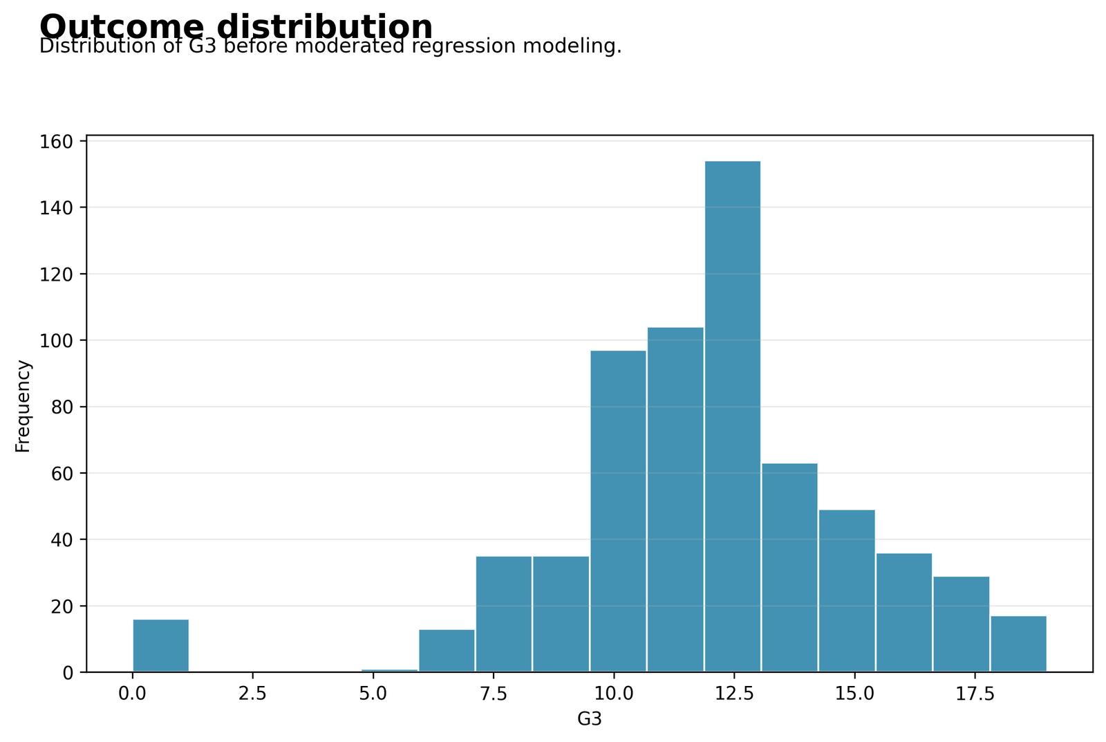
The histogram shows the distribution of final grade G3 before the interaction model is fitted. This Moderated Regression interpretation applies to the stated variables, coding and covariate adjustment.
For 649 students, G3 has mean 11.9060, SD 3.2307 and range 0–19.
Most final grades lie in the middle and upper range, but a small zero-grade subgroup is separated from the main distribution. Those zero scores are likely to create the largest prediction errors because their earlier grades often resemble students with nonzero outcomes. This Moderated Regression interpretation applies to the stated variables, coding and covariate adjustment.
Inspect zero-grade cases as a distinct substantive group and avoid relying on residual normality alone when judging the moderated model. This Moderated Regression interpretation applies to the stated variables, coding and covariate adjustment.
Chart 2: G1 and G3 by Studytime
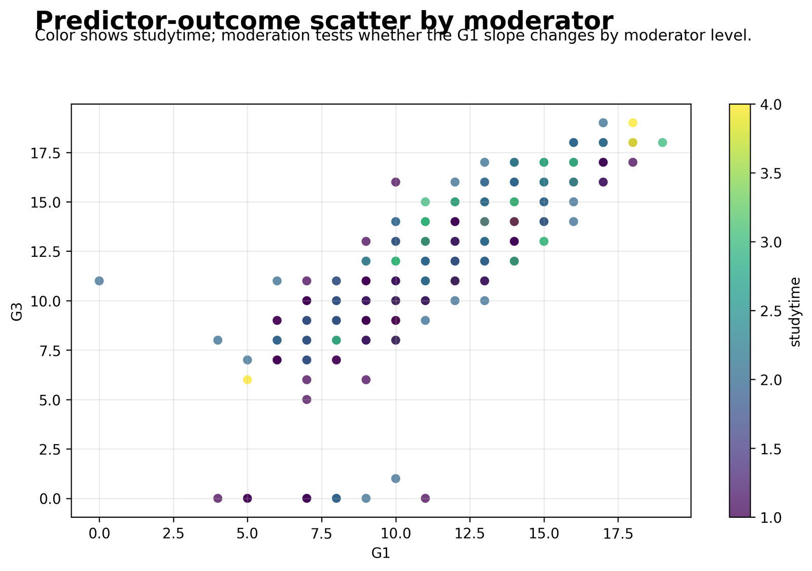
The scatterplot shows G1 against G3, with colour representing studytime from 1 to 4.
G1 and G3 both range from 0 to 19. The fitted interaction coefficient is −0.0464, p = .0340. This Moderated Regression interpretation applies to the stated variables, coding and covariate adjustment.
Students with higher G1 generally obtain higher G3 regardless of studytime. The studytime colours overlap heavily, so the moderator does not create separate grade clusters. It changes the slope only slightly: the G1–G3 relationship is somewhat steeper at lower studytime. This Moderated Regression interpretation applies to the stated variables, coding and covariate adjustment.
Describe moderation as a subtle change in the G1 slope, not as evidence that studytime groups have completely different outcome patterns. This Moderated Regression interpretation applies to the stated variables, coding and covariate adjustment.
Chart 3: Observed Versus Predicted G3
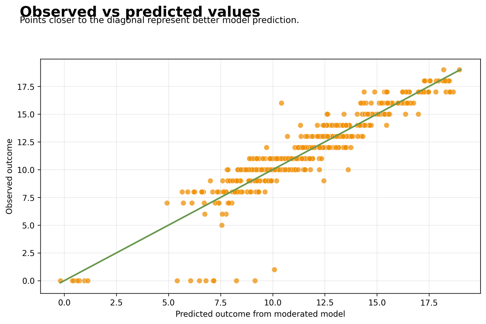
The chart compares actual G3 with predictions from the interaction model.
The moderated model has R² = 0.8534, adjusted R² 0.8507 and RMSE 1.2358.
The model reproduces ordinary grade outcomes very well because G2 and G1 contain strong academic information. Its most visible failures are zero-grade students whose predictor profiles lead to predicted values around 5–10. This Moderated Regression interpretation applies to the stated variables, coding and covariate adjustment.
Use the model for average prediction with caution around zero outcomes, and inspect whether zero indicates a distinct data-generating process. This Moderated Regression interpretation applies to the stated variables, coding and covariate adjustment.
Chart 4: Residuals Versus Predicted Values
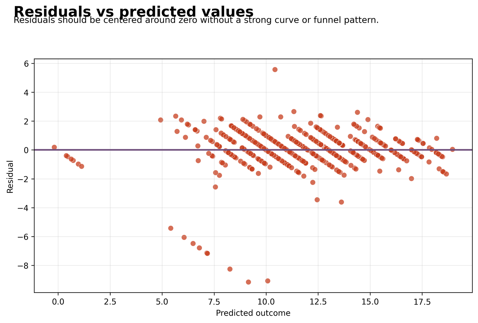
Residuals are plotted against the fitted G3 values to reveal systematic error patterns.
Most residuals fall between approximately −2 and +2, but several extend below −8 and one rises above +5. This Moderated Regression interpretation applies to the stated variables, coding and covariate adjustment.
The model is accurate for the dense central grade range but substantially overpredicts a small set of zero-grade students. The diagonal bands arise from integer-valued grades; the long negative tail is the more important problem. This Moderated Regression interpretation applies to the stated variables, coding and covariate adjustment.
Investigate the extreme negative residuals with studentized residuals, leverage and Cook’s distance, and report robust sensitivity results. This Moderated Regression interpretation applies to the stated variables, coding and covariate adjustment.
Chart 5: Coefficient Confidence Intervals
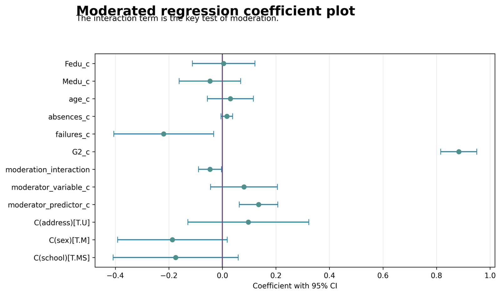
The coefficient plot compares adjusted slopes and their confidence intervals in the moderated model. This Moderated Regression interpretation applies to the stated variables, coding and covariate adjustment.
G1 = 0.1351, studytime = 0.0805, G1 × studytime = −0.0464, G2 = 0.8832 and failures = −0.2191. This Moderated Regression interpretation applies to the stated variables, coding and covariate adjustment.
Second-period grade explains most of the remaining variation in G3. G1 still contributes positively after G2 is controlled. The interaction is much smaller than the main academic effects, showing that moderation changes the G1 slope only slightly. This Moderated Regression interpretation applies to the stated variables, coding and covariate adjustment.
Separate statistical significance from magnitude: emphasize the strong G2 effect and describe the interaction as a small adjustment to the G1 relationship. This Moderated Regression interpretation applies to the stated variables, coding and covariate adjustment.
Chart 6: Moderation Interaction Plot
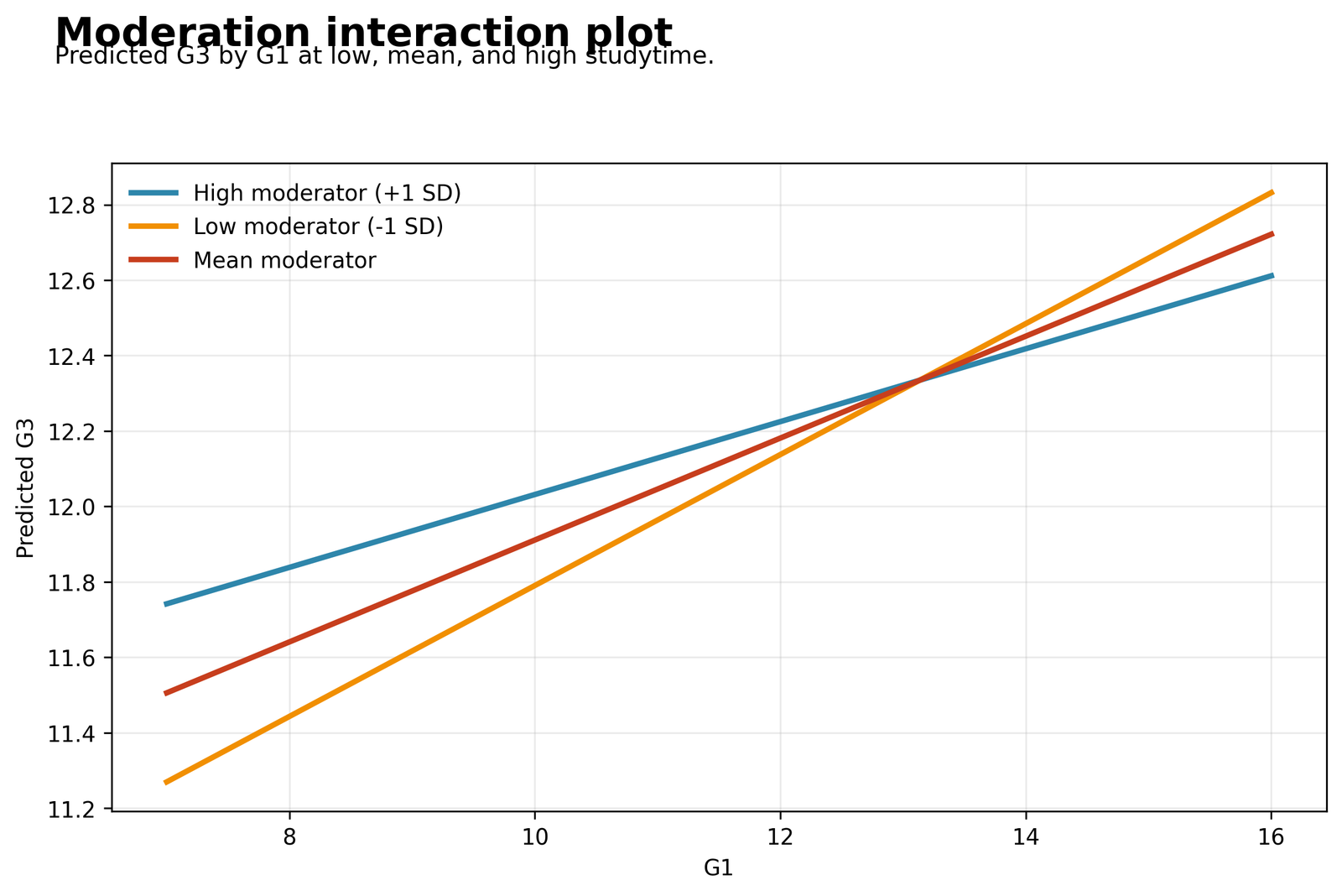
Predicted G3 is plotted across G1 for low, mean and high studytime.
The simple G1 slopes are 0.1735 at low studytime, 0.1351 at the mean and 0.0966 at high studytime. This Moderated Regression interpretation applies to the stated variables, coding and covariate adjustment.
G1 predicts higher G3 at every studytime level. At lower G1 values, high studytime slightly offsets weaker prior grades; at higher G1 values, the steeper low-studytime line overtakes it. The lines cross near the middle because the interaction is negative. This Moderated Regression interpretation applies to the stated variables, coding and covariate adjustment.
Do not say that high studytime lowers final grades. Say that the incremental association between G1 and G3 is weaker when studytime is higher, conditional on G2 and the controls. This Moderated Regression interpretation applies to the stated variables, coding and covariate adjustment.
Chart 7: Model-Fit Comparison
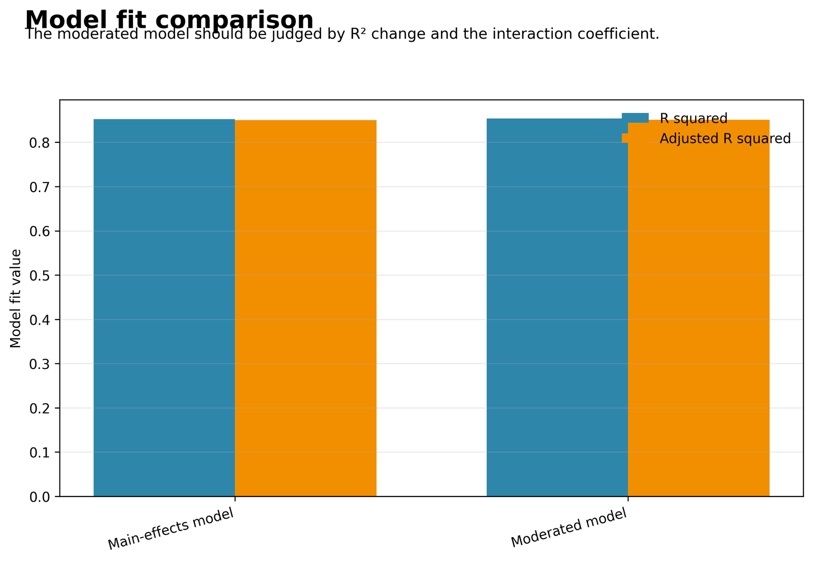
The bars compare R² and adjusted R² for the main-effects and moderated models.
R² rises from 0.8524 to 0.8534; ΔR² = 0.0010. F-change = 4.5120, p = .0340.
The interaction improves fit enough to be statistically detectable, but it explains only about one additional tenth of one percent of G3 variance. Almost all predictive performance was already present in the main effects and controls. This Moderated Regression interpretation applies to the stated variables, coding and covariate adjustment.
Report both the significant F-change and the tiny ΔR². Avoid presenting the interaction as a major improvement in prediction. This Moderated Regression interpretation applies to the stated variables, coding and covariate adjustment.
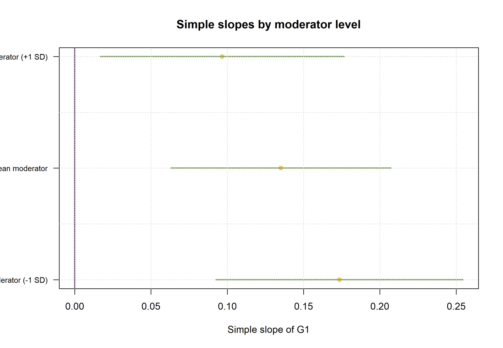
Chart 8: Simple Slopes of G1
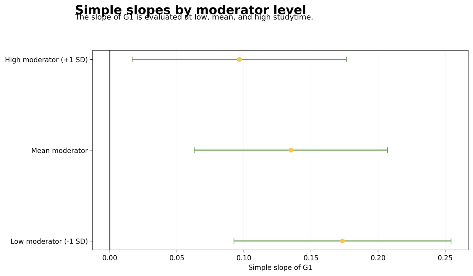
The forest plot shows the conditional G1 slope at low, mean and high studytime with 95% confidence intervals. This Moderated Regression interpretation applies to the stated variables, coding and covariate adjustment.
Low studytime: 0.1735, CI [0.0926, 0.2545]; mean: 0.1351, CI [0.0629, 0.2072]; high: 0.0966, CI [0.0167, 0.1765]. This Moderated Regression interpretation applies to the stated variables, coding and covariate adjustment.
A better G1 is associated with a better G3 for every studytime level. The relationship does not disappear at high studytime; it becomes less steep. High studytime partly narrows the difference between students with lower and higher G1 scores. This Moderated Regression interpretation applies to the stated variables, coding and covariate adjustment.
Conclude that studytime attenuates rather than reverses the G1 slope. Report all three slopes and their intervals, not only the interaction p-value.
R Charts: Two Charts Followed by Two Matching Explanation Boxes
Each R pair is followed by explanation boxes that describe the substantive process represented by the chart rather than simply repeating its values.
R Chart 1: Outcome Distribution for G3
Most final grades lie in the middle and upper range, but a small zero-grade subgroup is separated from the main distribution. Those zero scores are likely to create the largest prediction errors because their earlier grades often resemble students with nonzero outcomes.
R Chart 2: G1 and G3 by Studytime
Students with higher G1 generally obtain higher G3 regardless of studytime. The studytime colours overlap heavily, so the moderator does not create separate grade clusters. It changes the slope only slightly: the G1–G3 relationship is somewhat steeper at lower studytime.
R Chart 3: Observed Versus Predicted G3
The model reproduces ordinary grade outcomes very well because G2 and G1 contain strong academic information. Its most visible failures are zero-grade students whose predictor profiles lead to predicted values around 5–10.
R Chart 4: Residuals Versus Predicted Values
The model is accurate for the dense central grade range but substantially overpredicts a small set of zero-grade students. The diagonal bands arise from integer-valued grades; the long negative tail is the more important problem.
R Chart 5: Coefficient Confidence Intervals
Second-period grade explains most of the remaining variation in G3. G1 still contributes positively after G2 is controlled. The interaction is much smaller than the main academic effects, showing that moderation changes the G1 slope only slightly.
R Chart 6: Moderation Interaction Plot
G1 predicts higher G3 at every studytime level. At lower G1 values, high studytime slightly offsets weaker prior grades; at higher G1 values, the steeper low-studytime line overtakes it. The lines cross near the middle because the interaction is negative.
R Chart 7: Model-Fit Comparison
The interaction improves fit enough to be statistically detectable, but it explains only about one additional tenth of one percent of G3 variance. Almost all predictive performance was already present in the main effects and controls.
R Chart 8: Simple Slopes of G1
A better G1 is associated with a better G3 for every studytime level. The relationship does not disappear at high studytime; it becomes less steep. High studytime partly narrows the difference between students with lower and higher G1 scores.
Complete Moderated Regression Coefficient Results
| Term | B | SE | p | 95% CI | Interpretation |
|---|---|---|---|---|---|
| G1 centered | 0.1351 | 0.0367 | .0003 | 0.0629–0.2072 | Positive slope at mean studytime |
| studytime centered | 0.0805 | 0.0636 | .2064 | −0.0445–0.2055 | Main effect not significant |
| G1 × studytime | −0.0464 | 0.0218 | .0340 | −0.0892 to −0.0035 | G1 slope weakens as studytime rises |
| G2 centered | 0.8832 | 0.0342 | <.001 | 0.8160–0.9503 | Dominant positive control |
| failures centered | −0.2191 | 0.0950 | .0214 | −0.4056 to −0.0326 | Negative adjusted association |
| absences centered | 0.0167 | 0.0112 | .1349 | −0.0052–0.0386 | Not significant |
| school MS | −0.1744 | 0.1189 | .1429 | −0.4079–0.0591 | Not significant |
| sex male | −0.1866 | 0.1043 | .0741 | −0.3915–0.0182 | Not significant |
| address urban | 0.0972 | 0.1150 | .3985 | −0.1286–0.3230 | Not significant |
Simple slopes
| Studytime level | G1 slope | SE | p | 95% CI |
|---|---|---|---|---|
| Low (−1 SD) | 0.1735 | 0.0412 | <.001 | 0.0926–0.2545 |
| Mean | 0.1351 | 0.0367 | .0003 | 0.0629–0.2072 |
| High (+1 SD) | 0.0966 | 0.0407 | .0179 | 0.0167–0.1765 |
Report the interaction and confidence interval using the P-Value and Confidence Interval guides.
Simple Slopes and Practical Prediction
At lower studytime
- G1 slope = 0.1735
- Prior grade differences remain more visible
- Predicted lines are steeper
At higher studytime
- G1 slope = 0.0966
- G1 still predicts G3
- The grade gap is somewhat compressed
For two students who differ by one G1 point but have the same G2 and controls, the predicted G3 difference is about 0.174 at low studytime and 0.097 at high studytime. The difference between these slopes is statistically detectable but small.
Diagnostics and Model Choice
Regression diagnostics
- Check residual linearity and variance
- Review G1–G2 collinearity
- Inspect leverage and influence
- Use robust sensitivity inference
Observed limitations
- Zero-grade cases create large negative residuals
- Interaction adds only ΔR²=.0010
- Studytime has four ordinal categories
- Prediction is mainly driven by G2
Use Variance Inflation Factor, Tolerance Statistic, Studentized Residuals, Cook’s Distance and Influence Diagnostics. This Moderated Regression interpretation should be evaluated with the complete model specification and reported uncertainty.
Assess heteroskedasticity with residual plots and the Breusch-Pagan Test. Consider HC3 robust standard errors because the significance of a small interaction can be sensitive to standard-error assumptions.
SPSS, Python, R and Excel Workflows
Python
Fits main-effects and interaction OLS models, calculates F-change and evaluates simple slopes.
- Eight charts
- Interaction confidence interval
- R² and error comparison
R
Uses nested lm() models, anova() comparison and conditional-slope calculations.
- Same centered interaction structure
- Simple slopes and plots
- Robust covariance option
SPSS
Uses centered or standardized variables and hierarchical regression blocks.
- Main effects before interaction
- Collinearity and residual output
- Saved predictions
Excel
Uses the worked workbook to calculate centered inputs, interaction values, predictions and simple slopes.
- Coefficient and fit sheets
- Simple-slopes table
- Prediction calculator
Code: Expand Only the Software You Need
Python Moderated Regression code
import pandas as pd
import statsmodels.formula.api as smf
from statsmodels.stats.anova import anova_lm

df = pd.read_csv("dataset.csv")
for v in ["G1", "studytime", "G2", "failures",
          "absences", "age", "Medu", "Fedu"]:
    df[v + "_c"] = df[v] - df[v].mean()

df["G1_x_studytime"] = df["G1_c"] * df["studytime_c"]

main = smf.ols(
    "G3 ~ G1_c + studytime_c + G2_c + failures_c + "
    "absences_c + age_c + Medu_c + Fedu_c + "
    "C(school) + C(sex) + C(address)",
    data=df
).fit()

moderated = smf.ols(
    "G3 ~ G1_c * studytime_c + G2_c + failures_c + "
    "absences_c + age_c + Medu_c + Fedu_c + "
    "C(school) + C(sex) + C(address)",
    data=df
).fit()

print(anova_lm(main, moderated))
R Moderated Regression code
df <- read.csv("dataset.csv")
df$G1_c <- df$G1 - mean(df$G1)
df$studytime_c <- df$studytime - mean(df$studytime)

main <- lm(
  G3 ~ G1_c + studytime_c + G2 + failures + absences +
    age + Medu + Fedu + school + sex + address,
  data = df
)

moderated <- lm(
  G3 ~ G1_c * studytime_c + G2 + failures + absences +
    age + Medu + Fedu + school + sex + address,
  data = df
)

anova(main, moderated)
summary(moderated)
SPSS Moderated Regression syntax
DESCRIPTIVES VARIABLES=G1 studytime G2 failures absences age Medu Fedu /SAVE.
COMPUTE G1_c = G1 - 11.3990755.
COMPUTE studytime_c = studytime - 1.9306626.
COMPUTE G1_x_studytime = G1_c * studytime_c.
EXECUTE.

REGRESSION
 /DEPENDENT G3
 /METHOD=ENTER G1_c studytime_c G2 failures absences
               age Medu Fedu school_MS sex_M address_U
 /METHOD=ENTER G1_x_studytime
 /STATISTICS COEFF OUTS R ANOVA CHANGE CI(95) COLLIN
 /SAVE PRED RESID.
Excel Moderated Regression formulas
Centered G1       = G1 - mean_G1
Centered W        = studytime - mean_studytime
Interaction       = Centered_G1 * Centered_W
Predicted G3      = intercept + b1*G1c + b2*Wc +
                    b3*Interaction + controls
Simple slope      = b1 + b3*Wc
R2 change         = R2_moderated - R2_main
Advanced Interpretation and Extensions
What moderation means
Moderation means the expected change in G3 associated with G1 differs across studytime. It does not require separate groups or a significant studytime main effect. See Main Effects vs Interaction Effects. This Moderated Regression interpretation should be evaluated with the complete model specification and reported uncertainty.
Main effects versus interactions
Main effects are conditional when an interaction is present. The G1 coefficient is the slope at mean-centered studytime, and the studytime coefficient is the effect when centered G1 equals zero.
Mean centering
Mean centering moves the zero point to the sample mean. It improves interpretation but does not change the interaction p-value, fitted values or R².
Standardizing predictors
Standardization changes the unit to standard deviations and can help compare coefficients. It also changes the scale of the interaction term, so the transformation must be documented.
Product-term construction
The product term must be formed from the same centered or standardized variables used for the lower-order terms. Omitting the lower-order terms violates model hierarchy.
Simple slopes
Simple slopes evaluate the G1 effect at selected studytime values. The three reported slopes remain positive. See Simple Effects Analysis for interpretation principles.
Johnson-Neyman regions
The Johnson-Neyman method identifies the full moderator range where the G1 slope is statistically different from zero. It avoids limiting interpretation to ±1 SD.
Categorical moderators
A categorical moderator is represented with dummy or effect coding. The interaction then compares slopes across categories.
Multiple moderators
Multiple moderators require multiple product terms and theory-driven interpretation. Correlated moderators can make lower-order coefficients unstable.
Three-way interactions
A three-way interaction asks whether a two-way interaction changes across a second moderator. Interpretation requires conditional two-way effects and carefully planned plots.
Hierarchical entry
Hierarchical entry compares a main-effects model with an interaction model. The interaction should enter after all lower-order terms.
R-squared change
ΔR² quantifies the variance added by the interaction. Here it is 0.0010. Compare this with Adjusted R-Squared and information criteria.
Incremental effect size
Incremental f² can be calculated as ΔR² divided by 1 minus the full-model R². A statistically significant interaction can still have a very small incremental effect size.
Model hierarchy principle
The model hierarchy principle keeps all lower-order components of an interaction in the model even when their individual p-values exceed .05.
Conditional main effects
With an interaction, the G1 and studytime coefficients are conditional effects at the other variable’s centered zero point. They are not global average effects.
Plotting interactions
Interaction plots should use realistic moderator values, label covariate settings and avoid exaggerating small vertical differences with a narrow axis.
Multicollinearity
Review Variance Inflation Factor and Tolerance Statistic. Centering can reduce nonessential collinearity with the product term but cannot remove substantive overlap between G1 and G2.
Heteroskedasticity
Use residual plots and the Breusch-Pagan Test to assess unequal variance. Heteroskedasticity affects standard errors more directly than coefficients.
Residual non-normality
Inspect Q-Q Plot Normality Check and Shapiro-Wilk Test cautiously. With 649 observations, graphical magnitude matters more than a single normality p-value.
Influential observations
Use Cook’s Distance, leverage and Influence Diagnostics. The zero-grade students create the largest negative residuals.
Robust standard errors
HC3 or similar robust standard errors can be reported when heteroskedasticity is plausible. The interaction conclusion should be checked for robustness.
Bootstrapped interaction inference
Bootstrap confidence intervals can evaluate the interaction and simple slopes without relying entirely on normal-theory standard errors.
Power for interaction effects
Interaction effects are usually harder to detect than main effects. Use simulation and Statistical Power planning because the observed ΔR² is only 0.0010.
Moderation in logistic regression
Binary outcomes require a logit interaction in Generalized Linear Model form. The coefficient is a change in log odds and probability interaction is scale-dependent.
Moderation versus mediation
Moderation tests whether a slope changes. Mediation tests whether an effect operates through an intervening variable. Moderated mediation combines both questions.
Replication and transportability
Replicate the interaction, simple slopes and fit change in another cohort. A significant interaction from one sample may not transport when moderator distributions change.
APA-Style Reporting
The conditional G1 slope was positive at low studytime, B = 0.174, 95% CI [0.093, 0.255], at mean studytime, B = 0.135, 95% CI [0.063, 0.207], and at high studytime, B = 0.097, 95% CI [0.017, 0.177]. The full model explained 85.34% of G3 variance. This Moderated Regression interpretation should be evaluated with the complete model specification and reported uncertainty.
Report the small ΔR² with the significant p-value and confidence interval. State that the slope weakens rather than saying that studytime has a negative overall effect.
Publication Checklist and Common Mistakes
Include in the final report
- Outcome, predictor and moderator definitions
- Centering method
- Main-effects and moderated models
- Interaction B, SE, p and CI
- ΔR² and F-change
- Simple slopes and interaction plot
- Residual and influence checks
Avoid these errors
- Dropping lower-order terms
- Interpreting main effects globally
- Reporting only the interaction p-value
- Calling a tiny ΔR² a large improvement
- Interpreting line crossing as causal
- Ignoring zero-grade outliers
Use the Null and Alternative Hypothesis, Type I and Type II Error and Statistical Power guides when planning interaction tests.
Downloads
Frequently Asked Questions
What is Moderated Regression?
What is the outcome in this analysis?
What is the focal predictor?
What is the moderator?
Is the interaction significant?
How much variance does the interaction add?
Are the simple slopes significant?
What does the negative interaction mean?
Does high studytime reduce G3?
Why center G1 and studytime?
Must the moderator main effect be significant?
What is the difference from hierarchical regression?
What is the difference from mediation?
Why report ΔR²?
Can Moderated Regression prove causation?
How should Moderated Regression be reported?
Final Moderated Regression Conclusion
The analysis supports a statistically significant negative interaction between G1 and studytime. G1 remains positively associated with G3 at low, mean and high studytime, but the slope declines as studytime increases.
The interaction adds only 0.0010 to R², so its practical contribution is small relative to the strong G2 and G1 main effects. The result is best interpreted as a subtle compression of the G1–G3 relationship at higher studytime.

