
Two-Way ANOVA Interaction, Simple Main Effects and Cell Mean Interpretation
Simple Effects Analysis: Formula, Interpretation, SPSS, Python, R and Excel Guide
Simple Effects Analysis is used after a factorial ANOVA or two-way ANOVA when an interaction effect is present or when the researcher needs to understand how one factor works inside each level of another factor. Instead of interpreting only broad main effects, Simple Effects Analysis examines the effect of Factor A within each level of Factor B, and the effect of Factor B within each level of Factor A. This guide explains the method with interaction profile plots, cell means, simple main effects, pairwise comparisons, critical difference thresholds, SPSS workflow, Python charts, R validation, Excel formulas and APA reporting.
Quick Answer: Simple Effects Analysis Result
Simple Effects Analysis answers a more specific question than the ordinary main-effect table. A main effect asks whether a factor matters on average. A simple effect asks whether that factor matters within a specific level of another factor. This is especially important when an interaction is present because the effect of one factor may change depending on the level of the second factor.
In the worked example, the analysis is organized around two categorical factors and a continuous outcome. The interaction profile plot, simple effects charts, cell mean heatmap and pairwise comparison map are used together. The result should be reported as a cell-level story: which factor changes the outcome inside each subgroup, where the effect is strongest, and where the effect is weak or absent.
Final interpretation: Simple Effects Analysis should be reported when the interaction pattern shows that the difference between groups is not constant across the second factor. The correct conclusion is not just “Factor A was significant” or “Factor B was significant.” The correct conclusion explains where the factor difference appears, which simple comparisons are meaningful, and how the cell means support that interpretation.
Important reporting point: If an interaction is meaningful, do not rely only on marginal means. Marginal means can hide the real pattern. Use cell means, interaction plots, simple effects tables and pairwise comparisons within the relevant factor levels.
Table of Contents
- What Is Simple Effects Analysis?
- When to Use Simple Effects Analysis
- Simple Effects Analysis Formula
- Null and Alternative Hypotheses
- Dataset and Variables Used
- Two-Way ANOVA Context and Decision Table
- Python Chart-by-Chart Interpretation
- R Validation Chart
- SPSS, R, Python and Excel Workflows
- Code Blocks for Simple Effects Analysis
- APA Reporting Wording
- Common Mistakes
- Downloads and Resources
- Related Guides
- FAQs
What Is Simple Effects Analysis?
Simple Effects Analysis is a follow-up method used in factorial designs. It examines the effect of one independent variable at a particular level of another independent variable. In a two-way ANOVA, the model may include Factor A, Factor B and the A × B interaction. If the interaction is meaningful, the average main effect may be incomplete or misleading.
For example, Factor A may appear to have a modest average effect. But inside one level of Factor B, Factor A may have a strong effect, while inside another level of Factor B, Factor A may have little or no effect. Simple Effects Analysis separates those conditional effects so the interaction can be explained properly.
The method is sometimes called simple main effects analysis. The phrase means that the analyst is still studying a main effect, but only inside a specific condition. The result is usually reported with cell means, standard errors, confidence intervals, F tests or pairwise comparisons.
Simple definition: Simple Effects Analysis tests whether one factor affects the outcome separately within each level of another factor.
Before reading this guide, review factorial ANOVA, one-way ANOVA, ANOVA assumptions, effect size, eta squared, p-values and confidence intervals.
When to Use Simple Effects Analysis
Use Simple Effects Analysis when a factorial ANOVA includes two or more factors and the interpretation requires conditional comparisons. It is most commonly used after a significant or practically meaningful interaction effect.
| Use Simple Effects Analysis When | Why It Matters | Example Interpretation |
|---|---|---|
| The interaction is significant | The effect of one factor depends on the level of another factor. | Factor A may differ at one level of Factor B but not another. |
| Interaction lines are nonparallel | The profile plot suggests changing group differences. | Different slopes indicate conditional effects. |
| Marginal means hide the pattern | Averaging across the second factor can hide subgroup results. | Cell means are needed instead of only marginal means. |
| You need subgroup-specific reporting | Readers need to know exactly where differences occur. | Report simple effect of Factor A within each level of Factor B. |
When not to use it mechanically: If there is no interaction pattern and the research question is only about broad average differences, main effects may be enough. If the interaction is meaningful, however, main effects should not be the final interpretation.
Simple Effects Analysis Formula
In a two-way ANOVA, the general model is:
A simple effect of Factor A within a specific level of Factor B compares A-level means while holding B fixed:
A simple effect of Factor B within a specific level of Factor A compares B-level means while holding A fixed:
For an F-style simple effect test, the mean square for the simple effect is compared with the appropriate error term:
| Symbol | Meaning | Interpretation |
|---|---|---|
| A | First factor | The factor whose effect may change across levels of B. |
| B | Second factor | The moderator or conditioning factor for A. |
| A×B | Interaction term | Shows whether the effect of one factor depends on the other factor. |
| Cell mean | Mean inside one A–B combination | The main value used for simple effects interpretation. |
| MS error | Error mean square | The denominator used for F-style simple effects tests. |
Decision rule: A simple effect is meaningful when the difference among levels of one factor is statistically significant or practically important within a specific level of the other factor. The final report should name the level where the effect occurs.
Null and Alternative Hypotheses for Simple Effects Analysis
Simple Effects Analysis uses conditional hypotheses. The hypothesis is not only “Factor A has an effect.” It is “Factor A has an effect within this level of Factor B.”
| Simple Effect | Null Hypothesis | Alternative Hypothesis |
|---|---|---|
| Factor A within B level 1 | Means of A are equal when B = level 1. | At least one A mean differs when B = level 1. |
| Factor A within B level 2 | Means of A are equal when B = level 2. | At least one A mean differs when B = level 2. |
| Factor B within A level 1 | Means of B are equal when A = level 1. | At least one B mean differs when A = level 1. |
| Factor B within A level 2 | Means of B are equal when A = level 2. | At least one B mean differs when A = level 2. |
Decision for this example: The correct final decision should identify the specific factor level where the simple effect is present. The interaction profile, cell mean heatmap and pairwise comparison map should be used together so the conclusion matches the actual cell pattern.
Dataset and Variables Used
The worked example is structured as a two-factor ANOVA problem. The dependent variable is continuous. Factor A and Factor B are categorical predictors. The goal is to understand whether the effect of one factor changes across levels of the other factor.
| Item | Role in Simple Effects Analysis | What to Interpret |
|---|---|---|
| Dependent variable | Continuous outcome | The mean outcome inside each A × B cell. |
| Factor A | First categorical predictor | Its effect is tested within each level of Factor B. |
| Factor B | Second categorical predictor | Its effect is tested within each level of Factor A. |
| A × B interaction | Conditional pattern | Shows whether the effect of one factor depends on the other factor. |
| Cell means | Core interpretation values | Show the exact subgroup pattern behind the interaction. |
Simple Effects Analysis is easiest to understand when paired with factorial ANOVA, ANOVA in Python, ANOVA in R, ANOVA in SPSS, descriptive statistics, box plot interpretation and effect size.
Two-Way ANOVA Context and Simple Effects Decision Table
Simple Effects Analysis is normally interpreted after the two-way ANOVA table has been reviewed. The ANOVA table shows the main effect of Factor A, the main effect of Factor B and the A × B interaction. When the interaction is meaningful, the simple effects table becomes the main interpretation tool.
| ANOVA Term | Question Answered | How It Connects to Simple Effects |
|---|---|---|
| Main effect of Factor A | Does Factor A change the outcome on average? | May be incomplete if the A effect changes across B levels. |
| Main effect of Factor B | Does Factor B change the outcome on average? | May be incomplete if the B effect changes across A levels. |
| A × B interaction | Does the effect of one factor depend on the other factor? | If meaningful, simple effects explain exactly where the pattern occurs. |
| Simple effect of A within B | Does Factor A matter inside each B level? | Reports conditional A differences. |
| Simple effect of B within A | Does Factor B matter inside each A level? | Reports conditional B differences. |
Simple Effects Interpretation Summary
| Output Area | What It Shows | Final Reporting Use |
|---|---|---|
| Interaction profile plot | Whether lines are parallel, diverging, converging or crossing. | Explains why simple effects are needed. |
| Simple effects of A within B | Factor A differences separately for each level of B. | Reports where Factor A matters. |
| Simple effects of B within A | Factor B differences separately for each level of A. | Reports where Factor B matters. |
| Cell mean heatmap | Mean outcome inside every A × B cell. | Shows the exact subgroup pattern. |
| Pairwise comparison map | Which cell or level comparisons are strongest. | Prevents vague interaction reporting. |
Result summary: A strong Simple Effects Analysis report should tell the reader where the interaction occurs. It should not only say “the interaction was significant.” It should identify the factor levels, cell means, pairwise differences and the direction of the conditional effects.
Python Chart-by-Chart Interpretation
The Python charts show the complete Simple Effects Analysis workflow. They move from the interaction profile to simple effects of each factor, cell means, pairwise comparisons, critical difference thresholds, marginal versus cell means and distribution context.
Python Chart 1: Simple Effects Interaction Profile
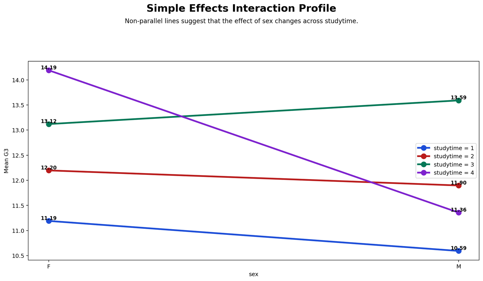
The interaction profile plot is the first chart to read. If the lines are parallel, the factor effects are similar across levels. If the lines separate, converge, cross or show different slopes, the chart suggests that one factor behaves differently depending on the level of the other factor.
This chart explains why Simple Effects Analysis is needed. The visible pattern should guide the follow-up tests. The final report should describe whether the interaction is ordinal, disordinal, crossing or mainly a difference in effect size across levels.
Python Chart 2: Simple Effects of Factor A Within Factor B
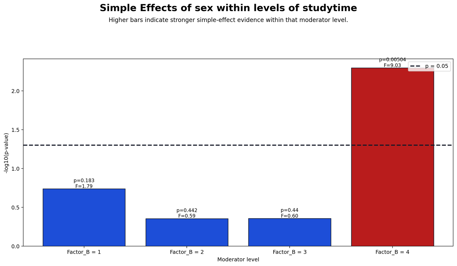
This chart isolates the effect of Factor A inside each level of Factor B. Instead of asking whether Factor A matters overall, it asks whether Factor A matters when B is held at a specific level.
The interpretation should name the B level where the Factor A difference is strongest. If Factor A is clear in one B level but weak in another, the interaction should be reported as a conditional Factor A effect.
Python Chart 3: Simple Effects of Factor B Within Factor A
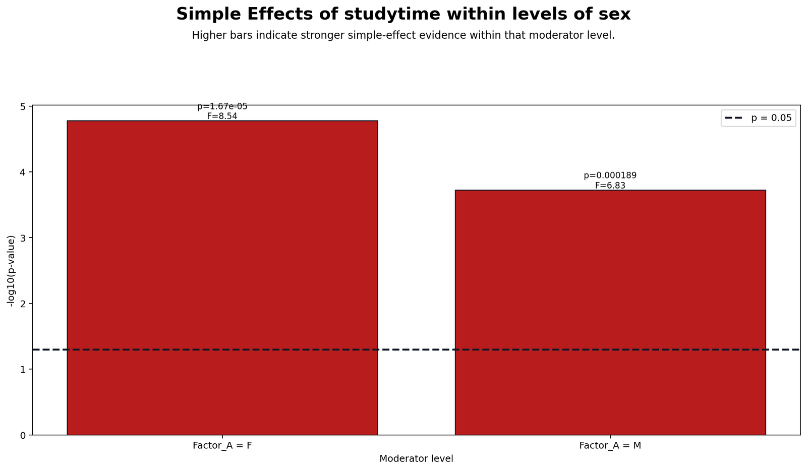
This chart reverses the conditioning direction. It tests the effect of Factor B inside each level of Factor A. This is important because an interaction can be explained from either direction, depending on the research question.
The best report chooses the direction that answers the research question most clearly. If the study asks how Factor B works for each group of Factor A, this chart becomes the main simple effects result.
Python Chart 4: Simple Effects Cell Mean Heatmap
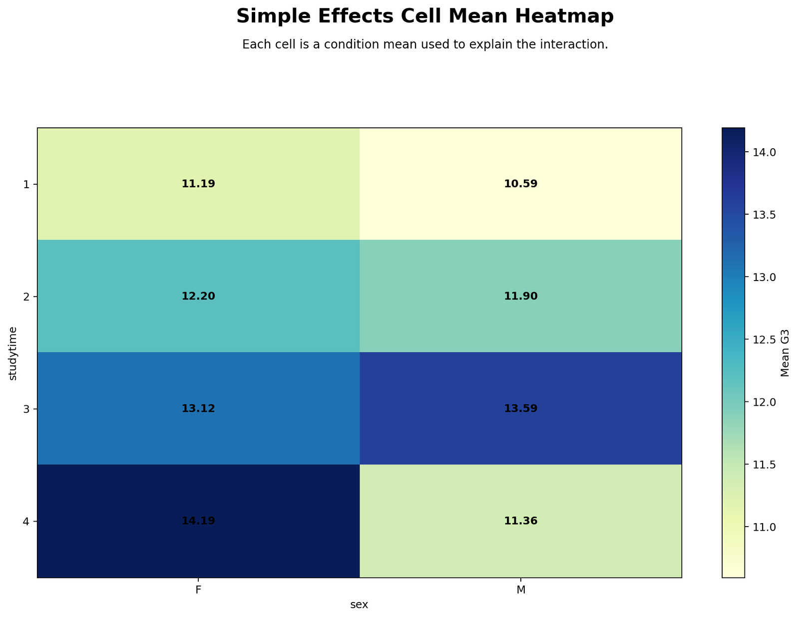
The cell mean heatmap gives the most direct view of the interaction. Each cell represents the mean outcome for one combination of Factor A and Factor B. Stronger or weaker cells show where the outcome is highest and lowest.
This chart prevents a common mistake: interpreting only marginal means. When an interaction exists, the cell means are often more important than the average main effects. The final explanation should match the cell mean pattern visible in this heatmap.
Python Chart 5: Simple Effect Pairwise Comparison Map
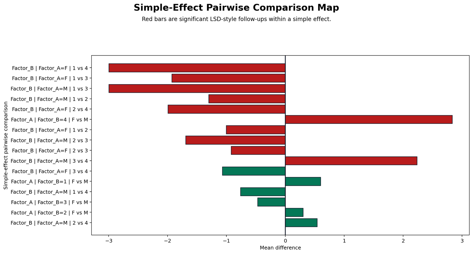
The pairwise comparison map shows which specific conditional comparisons are strongest. This is the chart that turns the interaction pattern into reportable differences. It helps identify which levels differ inside each simple effect test.
The final article should report these comparisons with direction. Instead of saying “there was a significant simple effect,” state which group had the higher mean and at which level of the other factor the difference occurred.
Python Chart 6: Simple Effect Critical Difference Thresholds
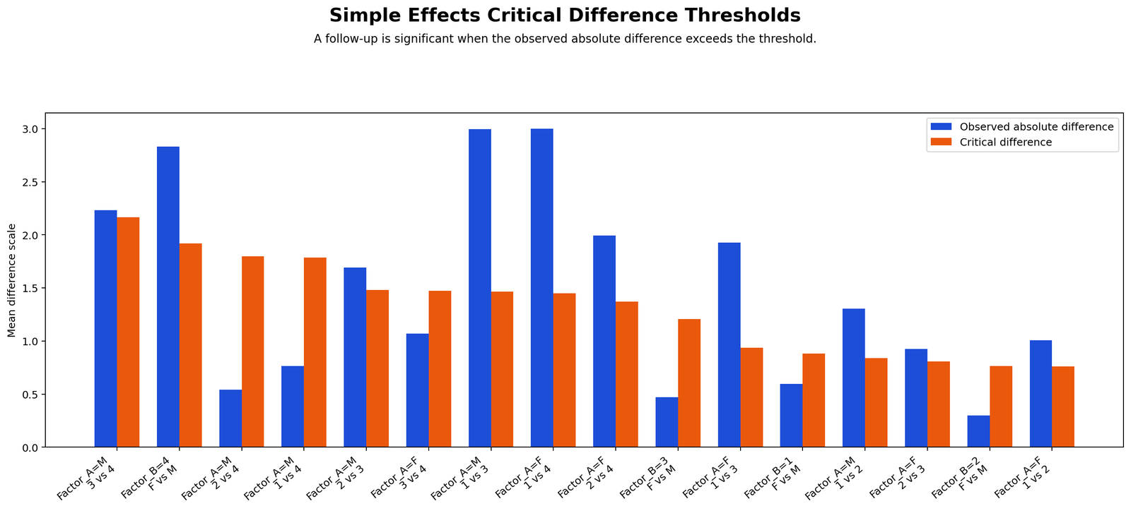
The critical difference chart shows whether observed conditional differences are large enough to pass the selected decision threshold. A difference may look visible in a mean chart, but the critical threshold helps determine whether it is strong enough statistically.
This chart is useful for avoiding overclaiming. If a difference is below the threshold, it can be described as small or descriptive, but it should not be reported as a statistically supported simple effect.
Python Chart 7: Marginal Means vs Cell Means
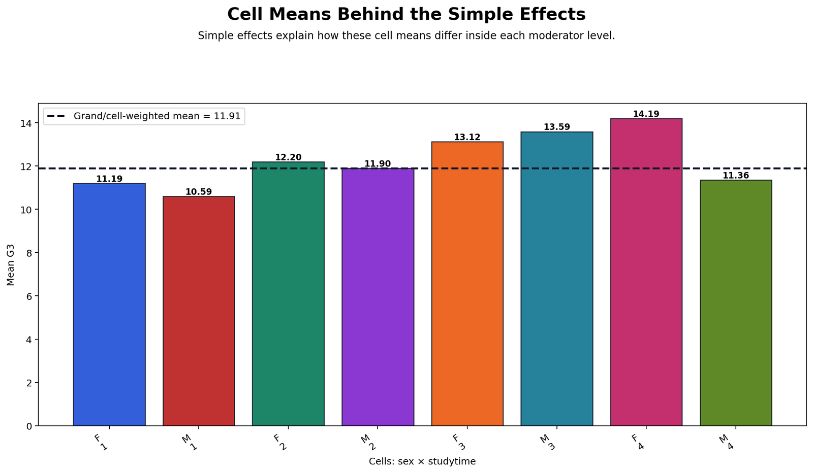
This chart explains why marginal means can be misleading when an interaction exists. Marginal means average across the second factor, while cell means show each subgroup combination. If the cell means move in different directions, the marginal mean can hide the real pattern.
The chart supports the main teaching point of Simple Effects Analysis: when the interaction is meaningful, cell-level interpretation is more informative than broad average interpretation.
Python Chart 8: Simple Effects Distribution Context
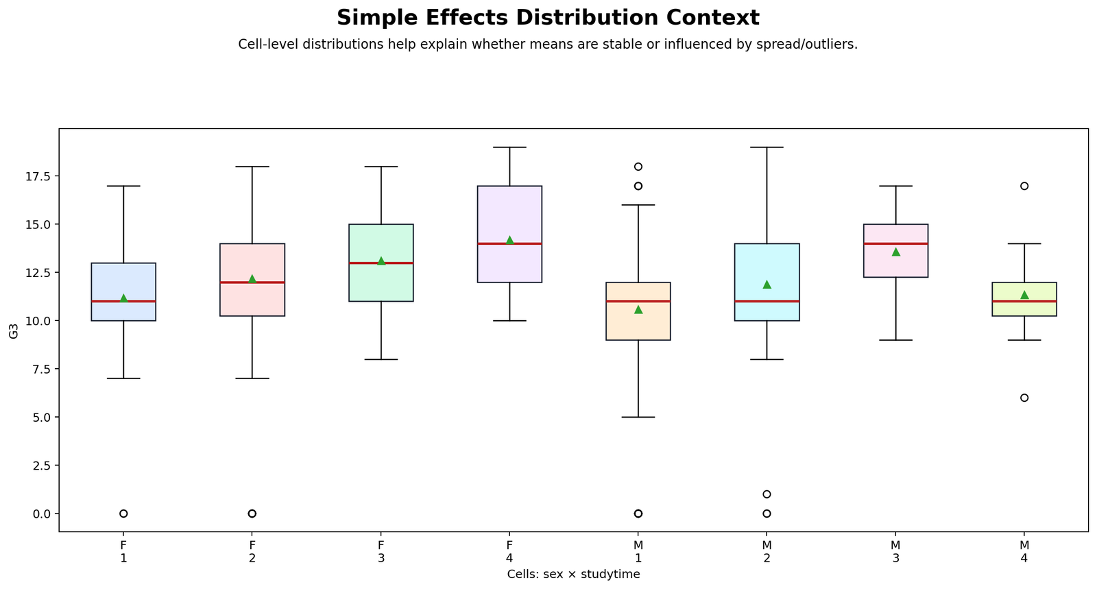
The distribution context chart shows the spread of scores inside the A × B cells. It helps readers understand whether cell mean differences are supported by compact distributions or whether there is large overlap.
This chart should be used before final reporting because simple effects are not only about mean height. They also depend on variability, sample size and overlap inside the cells.
R Validation Chart
The validation chart repeats the interaction profile in a second output set. It is useful for checking that the interaction pattern is not only a Python artifact and that the same visual structure appears in the validation workflow.
Validation Chart 1: Simple Effects Interaction Profile
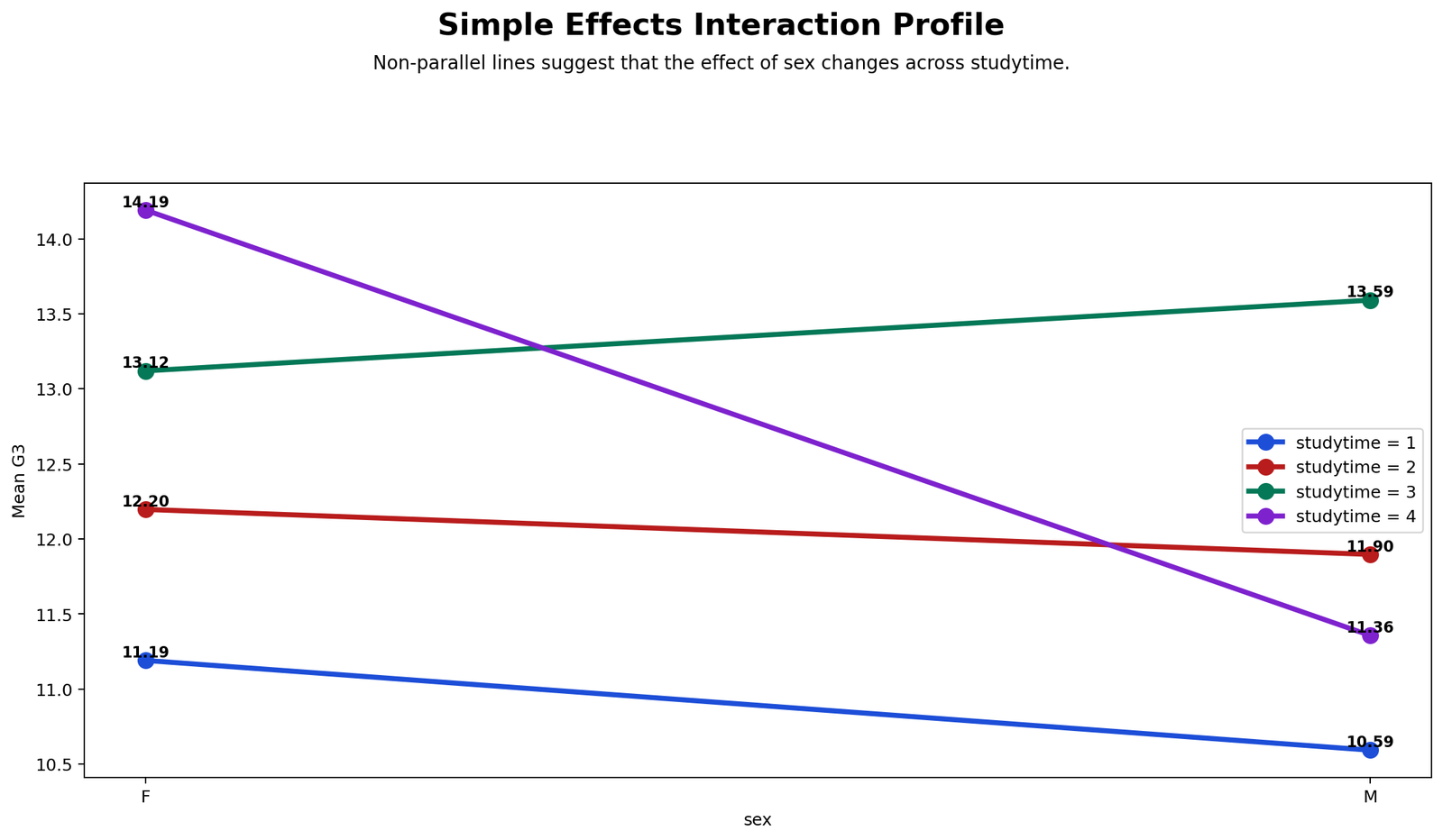
The validation interaction profile should be compared with the Python profile plot. If the same nonparallel or conditional pattern appears, it strengthens the conclusion that simple effects are needed.
This chart also helps confirm the direction of reporting. The final interpretation should explain the interaction through the factor direction that makes the profile easiest to understand.
SPSS, R, Python and Excel Workflows for Simple Effects Analysis
Simple Effects Analysis can be completed in SPSS, R, Python and Excel. SPSS is useful for estimated marginal means and pairwise comparisons. R and Python are best for reproducible model fitting, interaction plots, cell means and custom simple effects tables. Excel can calculate cell means and teach the logic, but full inferential testing is easier in statistical software.
SPSS Workflow
| Step | SPSS Action | Purpose |
|---|---|---|
| Open data | File > Open > Data | Load the dataset with outcome, Factor A and Factor B. |
| Run factorial ANOVA | Analyze > General Linear Model > Univariate | Set the outcome as dependent variable and enter Factor A and Factor B as fixed factors. |
| Add interaction | Model > Full factorial | Estimate A, B and A × B. |
| Request means | Estimated Marginal Means | Request A × B cell means and pairwise comparisons. |
| Interpret simple effects | Compare A within B and B within A | Report where each conditional effect occurs. |
R Workflow
| Step | R Action | Purpose |
|---|---|---|
| Read data | read.csv() | Import the dataset. |
| Fit interaction model | aov(outcome ~ factor_a * factor_b) | Estimate main effects and interaction. |
| Calculate cell means | aggregate() or emmeans() | Get means for every A × B cell. |
| Run simple effects | emmeans(..., pairwise ~ A | B) | Compare Factor A inside each level of Factor B. |
| Reverse direction | emmeans(..., pairwise ~ B | A) | Compare Factor B inside each level of Factor A. |
Python Workflow
| Step | Python Action | Purpose |
|---|---|---|
| Read data | pandas.read_csv() | Load outcome, Factor A and Factor B. |
| Fit ANOVA model | ols("outcome ~ C(A) * C(B)") | Estimate main effects and interaction. |
| Create ANOVA table | sm.stats.anova_lm() | Check A, B and A × B terms. |
| Calculate cell means | groupby(["A","B"]).mean() | Build the simple effects interpretation table. |
| Run conditional pairwise tests | Loop within each level of the conditioning factor | Compare levels only inside the relevant subgroup. |
Excel Workflow
Excel can support Simple Effects Analysis by calculating cell means, marginal means and simple mean differences. It is best for teaching the logic. For formal F tests, adjusted pairwise comparisons and interaction output, SPSS, R or Python is preferred.
| Excel Item | Formula Idea | Purpose |
|---|---|---|
| Cell mean | =AVERAGEIFS(outcome_range,A_range,A_level,B_range,B_level) | Calculate each A × B mean. |
| Cell count | =COUNTIFS(A_range,A_level,B_range,B_level) | Check sample size in each cell. |
| Simple effect of A within B | =CellMean_A1B1-CellMean_A2B1 | Compare Factor A levels while holding B fixed. |
| Simple effect of B within A | =CellMean_A1B1-CellMean_A1B2 | Compare Factor B levels while holding A fixed. |
| Marginal mean | =AVERAGEIF(A_range,A_level,outcome_range) | Compare broad main-effect means with cell means. |
Code Blocks for Simple Effects Analysis
SPSS Syntax
UNIANOVA outcome BY factor_a factor_b
  /METHOD = SSTYPE(3)
  /INTERCEPT = INCLUDE
  /PRINT = DESCRIPTIVE ETASQ HOMOGENEITY
  /EMMEANS = TABLES(factor_a*factor_b)
  /EMMEANS = TABLES(factor_a*factor_b) COMPARE(factor_a) ADJ(SIDAK)
  /EMMEANS = TABLES(factor_a*factor_b) COMPARE(factor_b) ADJ(SIDAK)
  /DESIGN = factor_a factor_b factor_a*factor_b.
R Code
data <- read.csv("dataset.csv")
data$factor_a <- factor(data$factor_a)
data$factor_b <- factor(data$factor_b)

# Two-way ANOVA with interaction

model <- aov(outcome ~ factor_a * factor_b, data = data)
summary(model)

# Cell means

aggregate(outcome ~ factor_a + factor_b, data = data, mean)

# Simple effects with emmeans

# install.packages("emmeans")

library(emmeans)

emm <- emmeans(model, ~ factor_a * factor_b)

# Effect of Factor A within each level of Factor B

pairs(emmeans(model, ~ factor_a | factor_b), adjust = "sidak")

# Effect of Factor B within each level of Factor A

pairs(emmeans(model, ~ factor_b | factor_a), adjust = "sidak")
Python Code
import pandas as pd
import itertools
from scipy import stats
import statsmodels.api as sm
import statsmodels.formula.api as smf
from statsmodels.stats.multitest import multipletests

df = pd.read_csv("dataset.csv")

df["factor_a"] = df["factor_a"].astype("category")
df["factor_b"] = df["factor_b"].astype("category")

# Two-way ANOVA with interaction

model = smf.ols("outcome ~ C(factor_a) * C(factor_b)", data=df).fit()
anova = sm.stats.anova_lm(model, typ=2)
print(anova)

# Cell means

cell_means = (
df.groupby(["factor_a", "factor_b"])["outcome"]
.agg(["count", "mean", "std"])
.reset_index()
)
print(cell_means)

# Simple effect of Factor A within each level of Factor B

rows_a_within_b = []

for b_level in df["factor_b"].cat.categories:
subset = df[df["factor_b"] == b_level]
a_levels = list(subset["factor_a"].cat.categories)

```
raw_p_values = []
comparisons = []

for a1, a2 in itertools.combinations(a_levels, 2):
    x1 = subset.loc[subset["factor_a"] == a1, "outcome"]
    x2 = subset.loc[subset["factor_a"] == a2, "outcome"]

    t_stat, raw_p = stats.ttest_ind(x1, x2, equal_var=True)
    raw_p_values.append(raw_p)
    comparisons.append((b_level, a1, a2, x1.mean() - x2.mean(), t_stat, raw_p))

if raw_p_values:
    reject, p_adj, _, _ = multipletests(raw_p_values, method="sidak")
    for item, adj_p, sig in zip(comparisons, p_adj, reject):
        rows_a_within_b.append(list(item) + [adj_p, sig])
```

a_within_b = pd.DataFrame(rows_a_within_b, columns=[
"factor_b_level", "factor_a_1", "factor_a_2",
"mean_difference", "t_statistic", "raw_p",
"sidak_adjusted_p", "significant"
])

print(a_within_b)

# Simple effect of Factor B within each level of Factor A

rows_b_within_a = []

for a_level in df["factor_a"].cat.categories:
subset = df[df["factor_a"] == a_level]
b_levels = list(subset["factor_b"].cat.categories)

```
raw_p_values = []
comparisons = []

for b1, b2 in itertools.combinations(b_levels, 2):
    x1 = subset.loc[subset["factor_b"] == b1, "outcome"]
    x2 = subset.loc[subset["factor_b"] == b2, "outcome"]

    t_stat, raw_p = stats.ttest_ind(x1, x2, equal_var=True)
    raw_p_values.append(raw_p)
    comparisons.append((a_level, b1, b2, x1.mean() - x2.mean(), t_stat, raw_p))

if raw_p_values:
    reject, p_adj, _, _ = multipletests(raw_p_values, method="sidak")
    for item, adj_p, sig in zip(comparisons, p_adj, reject):
        rows_b_within_a.append(list(item) + [adj_p, sig])
```

b_within_a = pd.DataFrame(rows_b_within_a, columns=[
"factor_a_level", "factor_b_1", "factor_b_2",
"mean_difference", "t_statistic", "raw_p",
"sidak_adjusted_p", "significant"
])

print(b_within_a)
Excel Formula Pattern
Cell mean:
=AVERAGEIFS(outcome_range,A_range,A_level,B_range,B_level)

Cell count:
=COUNTIFS(A_range,A_level,B_range,B_level)

Simple effect of A within B level 1:
=Mean_A1_B1-Mean_A2_B1

Simple effect of B within A level 1:
=Mean_A1_B1-Mean_A1_B2

Cell standard deviation:
=STDEV.S(FILTER(outcome_range,(A_range=A_level)*(B_range=B_level)))

Sidak adjusted p-value:
=1-(1-raw_p)^m

Decision:
=IF(adjusted_p<0.05,"Significant","Not significant")
APA Reporting Wording for Simple Effects Analysis
A two-way ANOVA was conducted to examine the effects of Factor A and Factor B on the outcome. Because the A × B interaction was meaningful, Simple Effects Analysis was used to interpret the conditional pattern. The simple effect of Factor A was examined separately within each level of Factor B, and the simple effect of Factor B was examined separately within each level of Factor A.
The simple effects results showed that the group differences were not uniform across all cells. The interaction profile and cell mean heatmap indicated that the size and direction of the effect changed across factor levels. Follow-up pairwise comparisons were used to identify which conditional differences were statistically meaningful. Therefore, the interaction should be reported using cell means and conditional comparisons rather than only marginal main effects.
Short APA version: Because the Factor A × Factor B interaction was meaningful, simple effects were examined. The results showed that the effect of one factor depended on the level of the other factor. Follow-up comparisons identified the specific cells where the conditional differences occurred.
Common Mistakes in Simple Effects Analysis
| Mistake | Why It Is a Problem | Better Practice |
|---|---|---|
| Reporting only main effects after an interaction | Main effects average across the other factor and can hide the real pattern. | Report simple effects and cell means. |
| Ignoring the interaction plot | The plot shows the shape of the conditional effect. | Use the profile plot before writing the result. |
| Using marginal means as the final result | Marginal means may be misleading when cell means differ strongly. | Use cell means for interaction interpretation. |
| Running too many unadjusted pairwise tests | Multiple testing increases false-positive risk. | Use Sidak, Bonferroni, Holm or another correction method. |
| Saying “there is an interaction” without explaining it | The reader still does not know where the effect occurs. | Name the specific factor levels where the simple effects appear. |
Most important warning: A significant interaction is not the final interpretation. It is the reason to perform Simple Effects Analysis. The final interpretation must explain the conditional pattern using cell means and follow-up comparisons.
Downloads and Resources
Use the downloadable Python report to verify the Simple Effects Analysis charts, interaction profile, cell means, pairwise comparison map, critical difference thresholds and distribution context.
FAQs About Simple Effects Analysis
What is Simple Effects Analysis?
Simple Effects Analysis is a follow-up method used after factorial ANOVA to test the effect of one factor within each level of another factor.
When should I use Simple Effects Analysis?
Use Simple Effects Analysis when an interaction effect is significant or meaningful and the main effects alone do not explain the full pattern.
What is the difference between main effects and simple effects?
A main effect averages across the other factor. A simple effect examines the effect of one factor within one specific level of the other factor.
Why are cell means important in Simple Effects Analysis?
Cell means show the actual subgroup means for each Factor A by Factor B combination. They reveal the pattern that marginal means may hide.
Can Simple Effects Analysis be done in SPSS?
Yes. In SPSS, use General Linear Model, request estimated marginal means for the interaction, and compare one factor within levels of the other factor.
Can Simple Effects Analysis be done in Excel?
Excel can calculate cell means, marginal means and simple mean differences. SPSS, R or Python is better for formal simple effects F tests and adjusted pairwise comparisons.
Should I report main effects when the interaction is significant?
You may report them for completeness, but the main interpretation should focus on the interaction and the simple effects because the effect of one factor depends on the other factor.

