
Factorial ANOVA, Marginal Means, Interaction Plots and Simple Effects
Main Effects vs Interaction Effects: Formula, Interpretation, SPSS, Python, R and Excel Guide
Main Effects vs Interaction Effects is one of the most important ideas in factorial ANOVA. A main effect tests whether one factor changes the outcome on average. An interaction effect tests whether the effect of one factor depends on the level of another factor. This guide explains Main Effects vs Interaction Effects using a two-way ANOVA example with SPSS output, Python charts, R validation, Excel workflow, formulas, simple effects, profile plots, APA reporting and downloadable resources.
Quick Answer: Main Effects vs Interaction Effects Result
The worked example uses a two-way factorial ANOVA with G3 final grade as the dependent variable. The two factors are sex as Factor A and studytime as Factor B. The model tests three questions at the same time: whether sex has an average effect on G3, whether studytime has an average effect on G3, and whether the effect of studytime changes depending on sex.
The most important decision is the interaction. The sex × studytime interaction was not statistically significant, with an interaction p-value around .083. This means the pattern of studytime differences was not strong enough to prove that it changes differently for females and males at α = .05. Because the interaction is not significant, the main effects can be interpreted more directly.
Final interpretation: Studytime is the clearest effect in this analysis. Average G3 scores increase across studytime levels, especially from the lowest studytime group to the higher studytime groups. The interaction is not significant, so the main studytime effect can be reported directly. The sex main effect is small and method-sensitive, so it should be reported with the exact software and sum-of-squares method used.
Important reporting point: Always check the interaction first. If the interaction is significant, main effects can become misleading because the effect of one factor depends on the other factor. If the interaction is not significant, as in this example, main effects are easier to interpret.
Table of Contents
- What Are Main Effects and Interaction Effects?
- When to Use Main Effects vs Interaction Effects
- Factorial ANOVA Formula
- Null and Alternative Hypotheses
- Dataset and Variables Used
- SPSS Output Interpretation
- Python Chart-by-Chart Interpretation
- R Chart-by-Chart Validation
- SPSS, R, Python and Excel Workflows
- Code Blocks for Main Effects vs Interaction Effects
- APA Reporting Wording
- Common Mistakes
- Downloads and Resources
- Related Guides
- FAQs
What Are Main Effects and Interaction Effects?
A main effect is the average effect of one factor on the dependent variable, ignoring the levels of the other factor. In this example, the main effect of studytime asks whether average G3 differs across the four studytime groups after accounting for sex and the two-way design. The main effect of sex asks whether average G3 differs between female and male students after accounting for studytime and the design.
An interaction effect asks whether the effect of one factor depends on another factor. In this example, the interaction asks whether the studytime pattern is different for females and males. If the lines in an interaction profile plot are strongly non-parallel or crossing, that may indicate an interaction. If the lines are roughly parallel, that usually suggests the main effects can be interpreted more directly.
The key rule is simple: interpret the interaction first. A significant interaction changes the meaning of main effects because the average effect may hide different subgroup patterns. A non-significant interaction means there is not enough evidence that the factors combine in a special way, so the analyst can focus more confidently on the main effects.
Simple definition: A main effect is an average difference for one factor. An interaction effect is a changing difference, where the effect of one factor depends on another factor.
Before interpreting main effects and interactions, review factorial ANOVA, t-test vs ANOVA, ANOVA assumptions, p-values, effect size, and eta squared.
When to Use Main Effects vs Interaction Effects
Use Main Effects vs Interaction Effects analysis when a study has at least two categorical independent variables and one continuous dependent variable. A two-way ANOVA is the simplest common example. The model estimates the effect of Factor A, the effect of Factor B, and the combined Factor A × Factor B effect.
| Use This Analysis When | Why It Matters | Example in This Guide |
|---|---|---|
| You have two or more factors | A factorial design can test each factor and their combination. | Factor A is sex and Factor B is studytime. |
| The outcome is continuous | ANOVA compares mean outcomes across groups. | G3 final grade is the dependent variable. |
| You want average factor effects | Main effects show average differences across levels of one factor. | Studytime has a clear average effect on G3. |
| You want to know whether factors combine | Interaction effects show whether one factor changes across another factor. | The sex × studytime interaction is not significant at α = .05. |
Best practice: Do not run separate one-way ANOVAs when a two-factor design is intended. A factorial ANOVA gives a cleaner answer because it tests main effects and the interaction in one model.
Factorial ANOVA Formula for Main Effects vs Interaction Effects
The two-way ANOVA model for this example can be written as:
Using the actual variables, the model is:
The main effect of Factor A tests average differences across levels of Factor A. The main effect of Factor B tests average differences across levels of Factor B. The interaction tests whether the effect of Factor A changes across Factor B, or equivalently, whether the effect of Factor B changes across Factor A.
| Model Term | Question It Answers | Interpretation in This Example |
|---|---|---|
| sex | Are average G3 scores different between females and males? | This effect is small and method-sensitive in the uploaded outputs. |
| studytime | Are average G3 scores different across studytime groups? | This is the clearest significant main effect. |
| sex × studytime | Does the studytime effect depend on sex? | The interaction is not significant at α = .05. |
| Error | How much variation remains unexplained by the model? | SPSS error mean square is approximately 9.676. |
Decision rule: For each model term, compare the p-value with α = .05. If p < .05, the term is statistically significant. If p ≥ .05, the term is not statistically significant.
Null and Alternative Hypotheses
Factorial ANOVA has a separate hypothesis for each main effect and for the interaction effect. The interaction hypothesis should be checked before the main-effect interpretation is finalized.
| Effect | Null Hypothesis | Alternative Hypothesis | Decision in This Example |
|---|---|---|---|
| Main effect of sex | Mean G3 is equal across sex groups. | Mean G3 differs across sex groups. | Small and method-sensitive; report the exact software/sum-of-squares method. |
| Main effect of studytime | Mean G3 is equal across studytime groups. | At least one studytime group mean differs. | Significant. |
| Interaction effect | The studytime pattern is the same across sex groups. | The studytime pattern changes across sex groups. | Not significant at α = .05. |
Decision for this example: The interaction is not significant, so the article focuses on the studytime main effect. Studytime is clearly related to G3, while the sex effect is small and should be reported cautiously because Type-II and Type-III workflows can produce different p-values in an unbalanced design.
Dataset and Variables Used
The worked example uses a student performance dataset. The dependent variable is G3 final grade. Factor A is sex, with female and male groups. Factor B is studytime, with four weekly study-time categories. The model tests whether G3 changes by sex, by studytime, and by the sex × studytime combination.
| Variable | Role | How It Is Used |
|---|---|---|
| G3 | Dependent variable | The final grade score being compared across factorial ANOVA cells. |
| sex | Factor A | Two-level factor used to test the sex main effect and the interaction. |
| studytime | Factor B | Four-level factor used to test the studytime main effect and the interaction. |
| sex × studytime | Interaction term | Tests whether the studytime pattern differs between female and male students. |
Cell Means Used in the Factorial Design
| Sex | Studytime | N | Mean G3 | Std. Deviation | Interpretation |
|---|---|---|---|---|---|
| Female | < 2 hours | 89 | 11.19 | 2.969 | Lowest female studytime cell. |
| Female | 2 to 5 hours | 198 | 12.20 | 3.224 | Higher than the lowest female studytime group. |
| Female | 5 to 10 hours | 75 | 13.12 | 2.610 | High female studytime cell. |
| Female | > 10 hours | 21 | 14.19 | 2.874 | Highest female cell mean. |
| Male | < 2 hours | 123 | 10.59 | 3.377 | Lowest male studytime cell. |
| Male | 2 to 5 hours | 107 | 11.90 | 3.285 | Middle male studytime cell. |
| Male | 5 to 10 hours | 22 | 13.59 | 2.108 | Highest male cell mean. |
| Male | > 10 hours | 14 | 11.36 | 2.499 | Smallest cell; lower than expected from the female pattern. |
Before interpreting this two-way ANOVA, review the cell counts and distribution shapes. Helpful related guides include descriptive statistics, box plot interpretation, Levene test, and ANOVA in SPSS.
SPSS Output Interpretation for Main Effects vs Interaction Effects
The SPSS output provides the official factorial ANOVA table, cell counts, cell descriptives, Levene test, tests of between-subjects effects and simple-effects context. The model is G3 = sex + studytime + sex × studytime.
SPSS Cell Counts
| Studytime Group | Female N | Male N | Total N | Balance Interpretation |
|---|---|---|---|---|
| < 2 hours | 89 | 123 | 212 | Large enough in both sex groups. |
| 2 to 5 hours | 198 | 107 | 305 | Largest studytime level overall. |
| 5 to 10 hours | 75 | 22 | 97 | Unbalanced between sex groups. |
| > 10 hours | 21 | 14 | 35 | Smallest studytime level; interpret cell means carefully. |
SPSS Levene Test
| Levene Version | Statistic | df1 | df2 | p-value | Interpretation |
|---|---|---|---|---|---|
| Based on mean | 0.719 | 7 | 641 | .656 | Not significant; no strong equal-variance warning. |
| Based on median | 0.733 | 7 | 641 | .644 | Also supports the variance assumption. |
| Based on trimmed mean | 0.720 | 7 | 641 | .656 | No strong variance problem indicated. |
SPSS Tests of Between-Subjects Effects
| Source | Type III SS | df | Mean Square | F | Sig. | Partial Eta Squared | Decision |
|---|---|---|---|---|---|---|---|
| Corrected Model | 560.961 | 7 | 80.137 | 8.282 | < .001 | .083 | The overall factorial ANOVA model is significant. |
| sex | 50.217 | 1 | 50.217 | 5.190 | .023 | .008 | Small significant effect in SPSS Type III output. |
| studytime | 382.980 | 3 | 127.660 | 13.193 | < .001 | .058 | Significant main effect. |
| sex × studytime | 64.815 | 3 | 21.605 | 2.233 | .083 | .010 | Not significant. |
| Error | 6202.306 | 641 | 9.676 | Residual variation after model terms. |
Type-II vs Type-III Reporting Note
The uploaded outputs show an important teaching point. In an unbalanced factorial design, the p-value for a main effect can depend on the sum-of-squares method and software workflow. The studytime main effect and the interaction conclusion are stable across the uploaded outputs. The sex main effect is smaller and more sensitive, so it should be reported with the exact method used.
| Effect | Python Type-II Style Output | SPSS Type-III Output | Practical Reporting |
|---|---|---|---|
| sex | F ≈ 3.211, p ≈ .0736 | F = 5.190, p = .023 | Small, method-sensitive effect; report method. |
| studytime | F ≈ 13.210, p < .001 | F = 13.193, p < .001 | Clear significant main effect. |
| sex × studytime | F ≈ 2.233, p ≈ .083 | F = 2.233, p = .083 | Not significant at α = .05. |
Simple Effects Context
Simple effects are most important when the interaction is significant or when the analyst has a planned reason to examine subgroup patterns. In this example, studytime differs within females and within males. Sex differs clearly only inside the highest studytime group, but because the overall interaction is not significant at α = .05, these simple-effect results should be treated as supporting context rather than the main headline.
| Simple Effect Question | F | p-value | Decision |
|---|---|---|---|
| Does studytime differ within females? | 8.545 | < .001 | Significant. |
| Does studytime differ within males? | 6.834 | < .001 | Significant. |
| Does sex differ within studytime group 1? | 1.786 | .183 | Not significant. |
| Does sex differ within studytime group 2? | 0.593 | .442 | Not significant. |
| Does sex differ within studytime group 3? | 0.600 | .440 | Not significant. |
| Does sex differ within studytime group 4? | 9.029 | .005 | Significant, but based on the smallest studytime cell. |
SPSS interpretation summary: The overall factorial model is significant, the Levene test does not show a strong variance problem, the studytime main effect is significant, and the sex × studytime interaction is not significant. The practical conclusion is that studytime is the clearest factor associated with G3 in this two-way ANOVA.
Python Chart-by-Chart Interpretation
The Python charts show the full workflow for explaining Main Effects vs Interaction Effects. They begin with an ANOVA report card, then show marginal means, interaction patterns, cell means, balance, simple effects, effect decomposition and cell distributions.
Python Chart 1: Main vs Interaction Effect Report Card
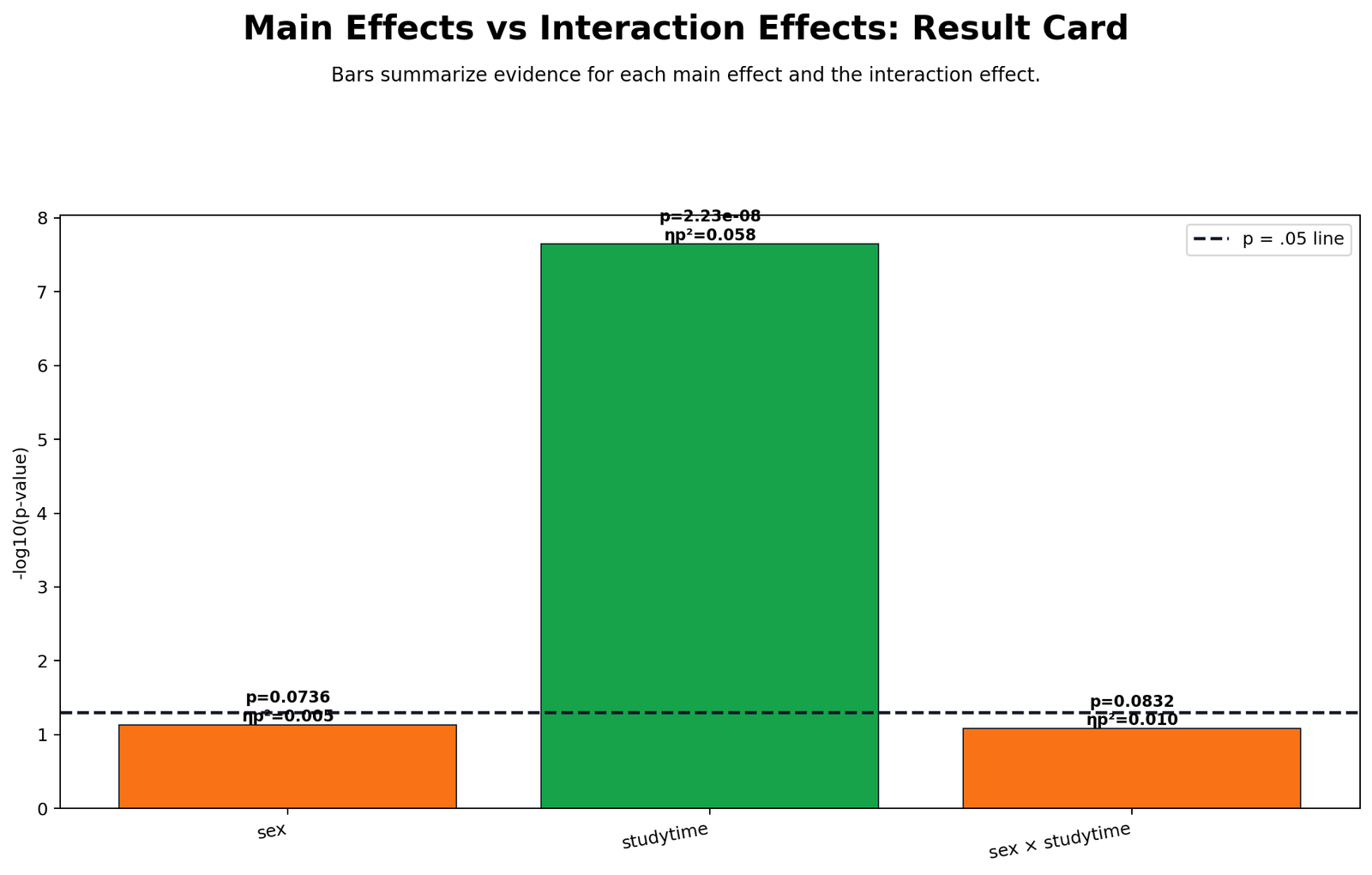
The report card gives the fastest summary of the factorial ANOVA. It shows that studytime is the main significant factor, while the sex × studytime interaction is not significant at α = .05. This means the main studytime effect can be interpreted without making the interaction the central conclusion.
The chart also reinforces the correct interpretation order. Interaction should be checked before main effects because a strong interaction can change the meaning of average differences. Here the interaction does not reach significance, so the main effect of studytime becomes the main story.
Python Chart 2: Main Effect Marginal Means for Factor A
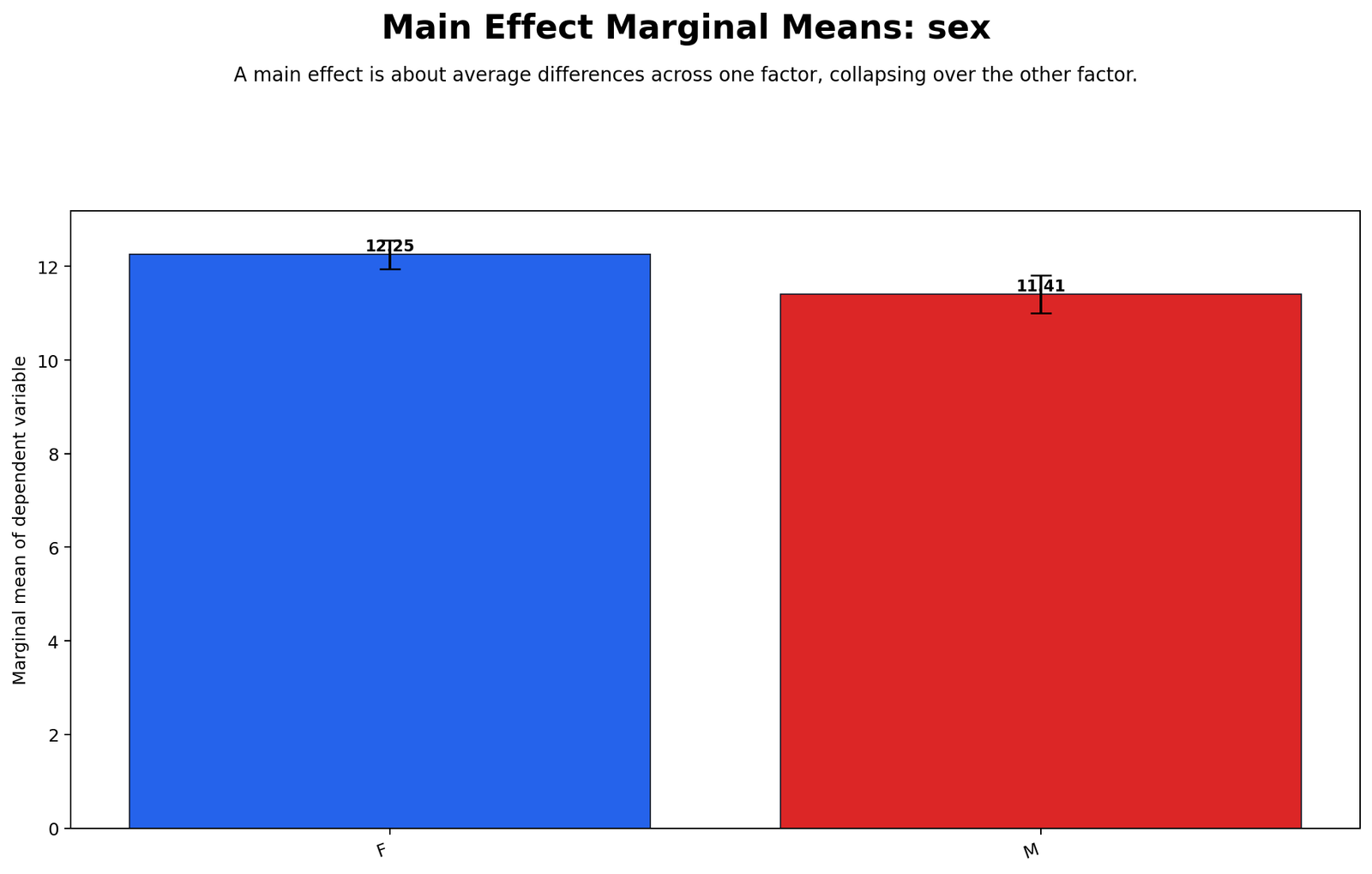
The Factor A marginal means chart compares average G3 between sex groups. Female students have a higher marginal mean than male students in the raw marginal summary. However, this effect is smaller than the studytime effect and is sensitive to the sum-of-squares method used in an unbalanced design.
This chart should therefore be interpreted cautiously. It is useful for showing the average sex difference, but the article should not overstate it. The strongest and most stable result across the analysis is still the studytime main effect.
Python Chart 3: Main Effect Marginal Means for Factor B
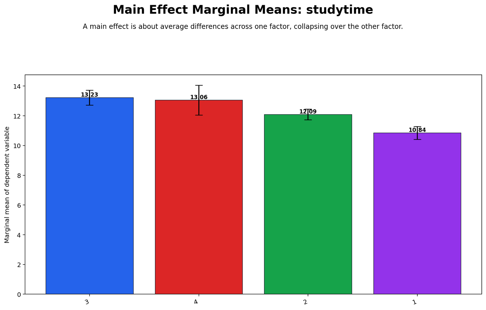
The Factor B marginal means chart shows the clearest pattern. The lowest studytime group has the lowest mean G3 score, while the higher studytime groups have higher means. Studytime group 3 has the highest average, and group 4 is also high but has a smaller sample size.
This chart supports the significant main effect of studytime. It shows that average G3 changes across studytime levels, even after the factorial design is considered.
Python Chart 4: Interaction Profile Plot
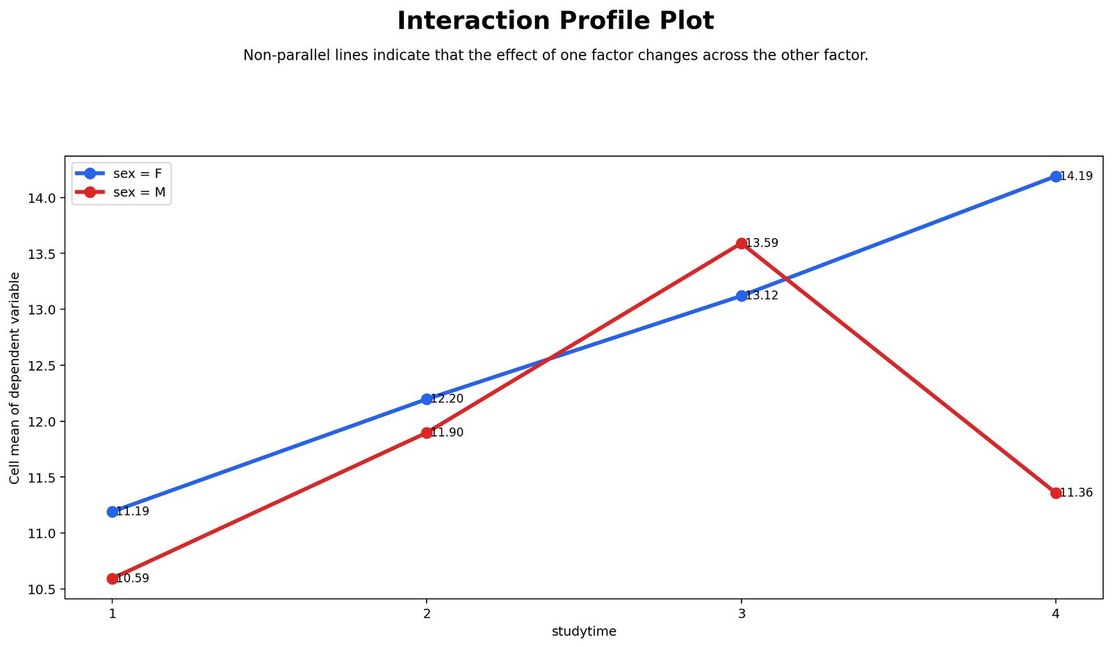
The interaction profile plot is the most important chart for judging whether the factors combine. The female and male lines show broadly similar improvement across studytime, although the highest studytime cell differs visually. Because the interaction p-value is around .083, this visual difference is not strong enough to declare a significant interaction at α = .05.
The plot should be reported carefully. It suggests a possible pattern worth noticing, especially in the highest studytime cell, but the statistical test does not support a firm interaction conclusion.
Python Chart 5: Interaction Cell Mean Heatmap
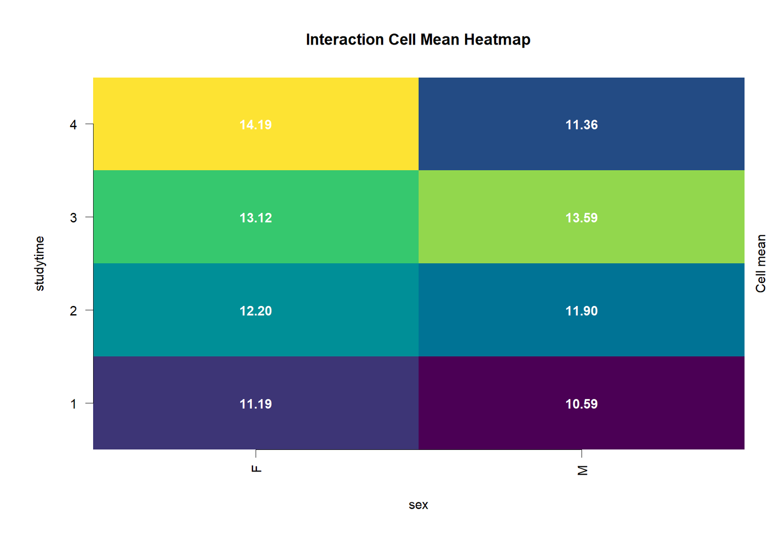
The cell mean heatmap shows the average G3 score in each factorial cell. The highest female cell is the female group with more than 10 hours of studytime. The male group with 5 to 10 hours also has a high mean, while the male group with more than 10 hours is lower.
This cell pattern explains why the interaction plot has some non-parallel behavior. However, the heatmap must be read with the balance map because some cells are small, especially the highest studytime cells.
Python Chart 6: Cell Size Balance Map
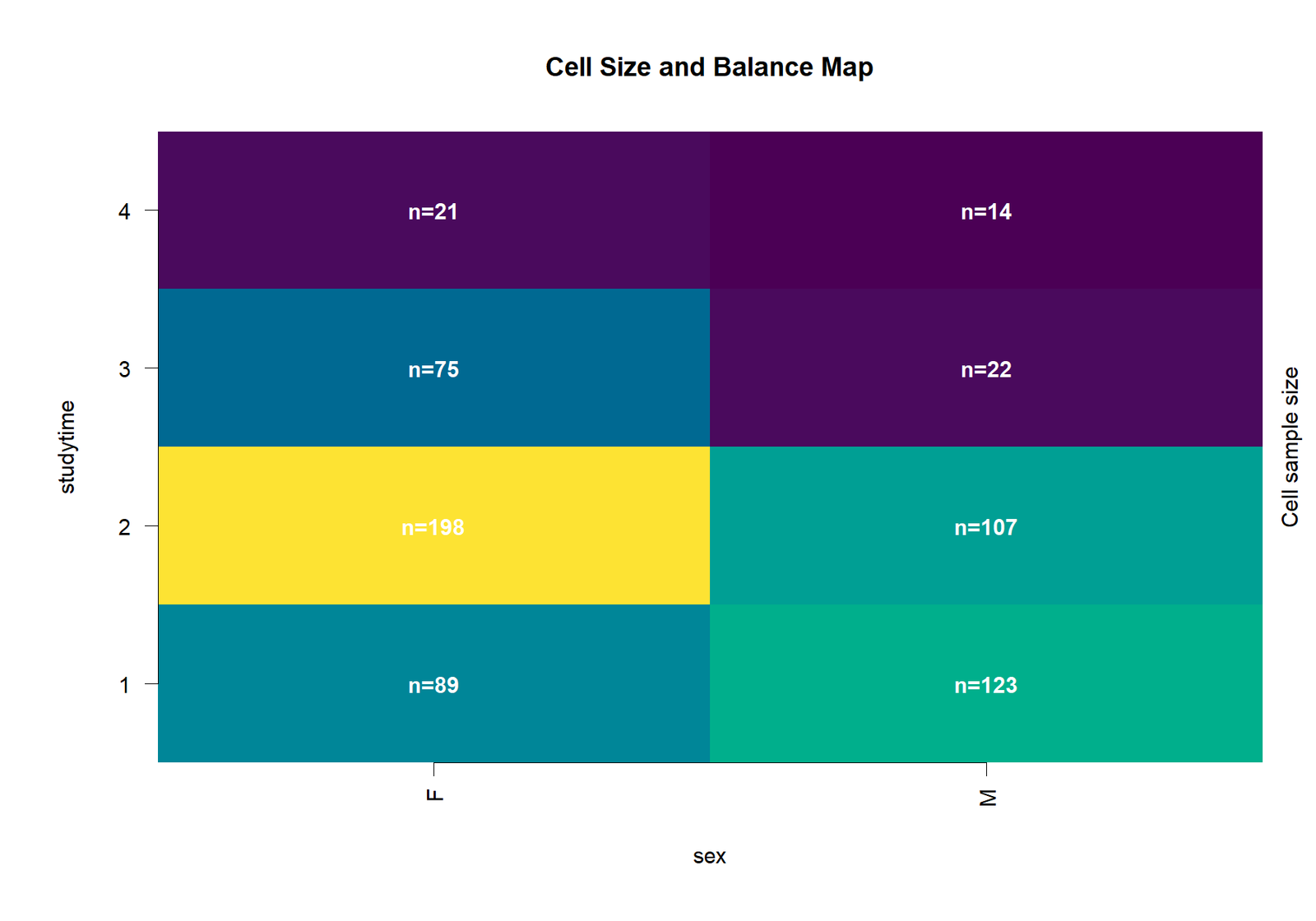
The balance map shows that the factorial design is not perfectly balanced. The 2 to 5 hours group has many cases, while the highest studytime cells have far fewer cases. This matters because small cells can make cell means less stable and can affect the interpretation of interaction patterns.
This chart explains why the sex main effect can be method-sensitive across Type-II and Type-III output. In unbalanced factorial ANOVA, the analyst must report the method clearly and should avoid exaggerated conclusions based on small cells.
Python Chart 7: Simple Effects p-values
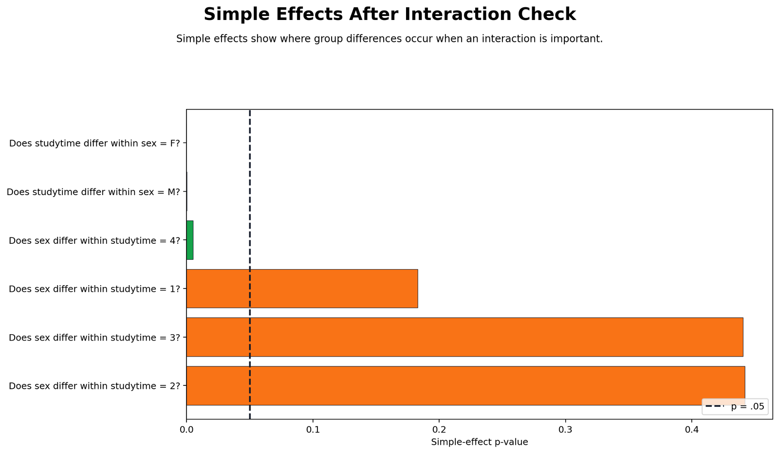
The simple effects chart shows that studytime differs within females and within males. It also shows that sex differences are not significant within the first three studytime groups but are significant within the highest studytime group.
Because the overall interaction is not significant, these simple effects should be treated as supporting detail rather than the central conclusion. The main report should prioritize the studytime main effect and describe the simple effects as exploratory or contextual.
Python Chart 8: Effect Decomposition Sum of Squares
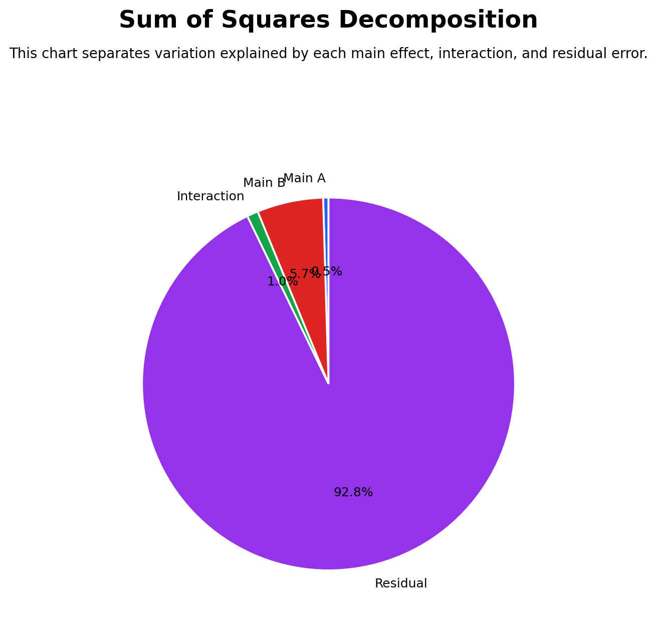
The effect decomposition chart shows how much variation is associated with each model term. Studytime accounts for more model sum of squares than sex or the interaction. The residual error remains the largest part of total variation because student performance depends on many variables beyond sex and studytime.
This chart is useful for effect-size interpretation. A statistically significant effect can still explain a modest portion of total variation, so the article should report both p-values and practical size.
Python Chart 9: Distribution by Interaction Cell
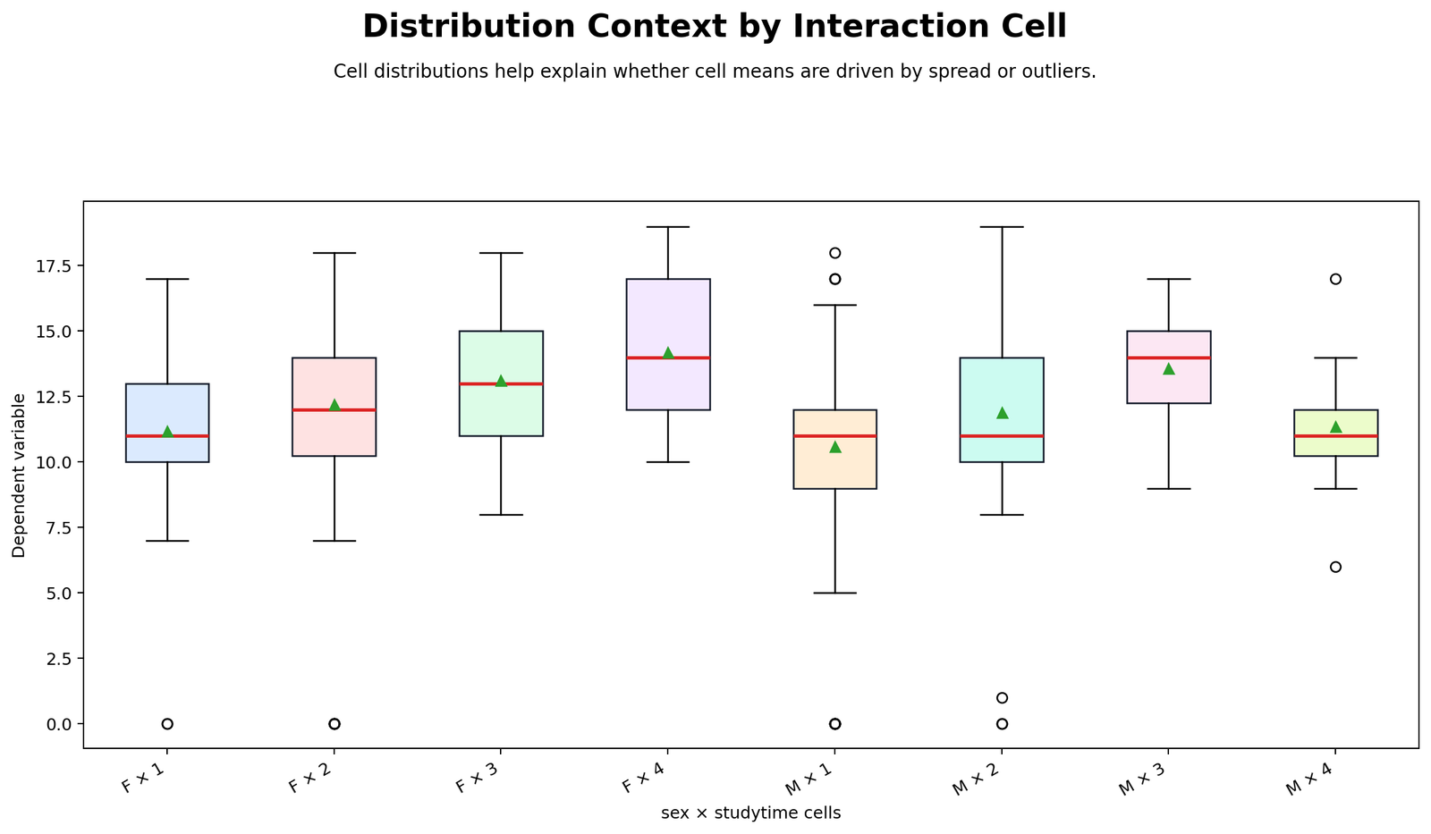
The distribution-by-cell chart shows the spread of G3 scores inside each factorial cell. It confirms that some cells have more spread and some cells have fewer observations. These distribution differences help explain why visual cell means should not be interpreted alone.
The chart supports a balanced conclusion: studytime has a clear average relationship with G3, but cell-level interaction claims require caution because the interaction test is not significant and some cells are small.
R Chart-by-Chart Validation
The R charts validate the same interpretation using a separate workflow. They confirm the studytime main effect pattern, the non-significant interaction conclusion, the cell mean structure, the balance issue and the need to report factorial ANOVA results carefully.
R Chart 1: Main vs Interaction Effect Report Card
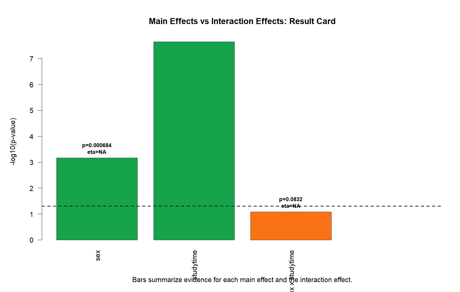
The R report card confirms that the interaction is not significant at α = .05. This keeps the interpretation focused on main effects rather than forcing a simple-effects-only explanation.
The chart also shows the same broad conclusion that studytime is an important factor. This supports the Python and SPSS interpretation.
R Chart 2: Main Effect Marginal Means for Factor A
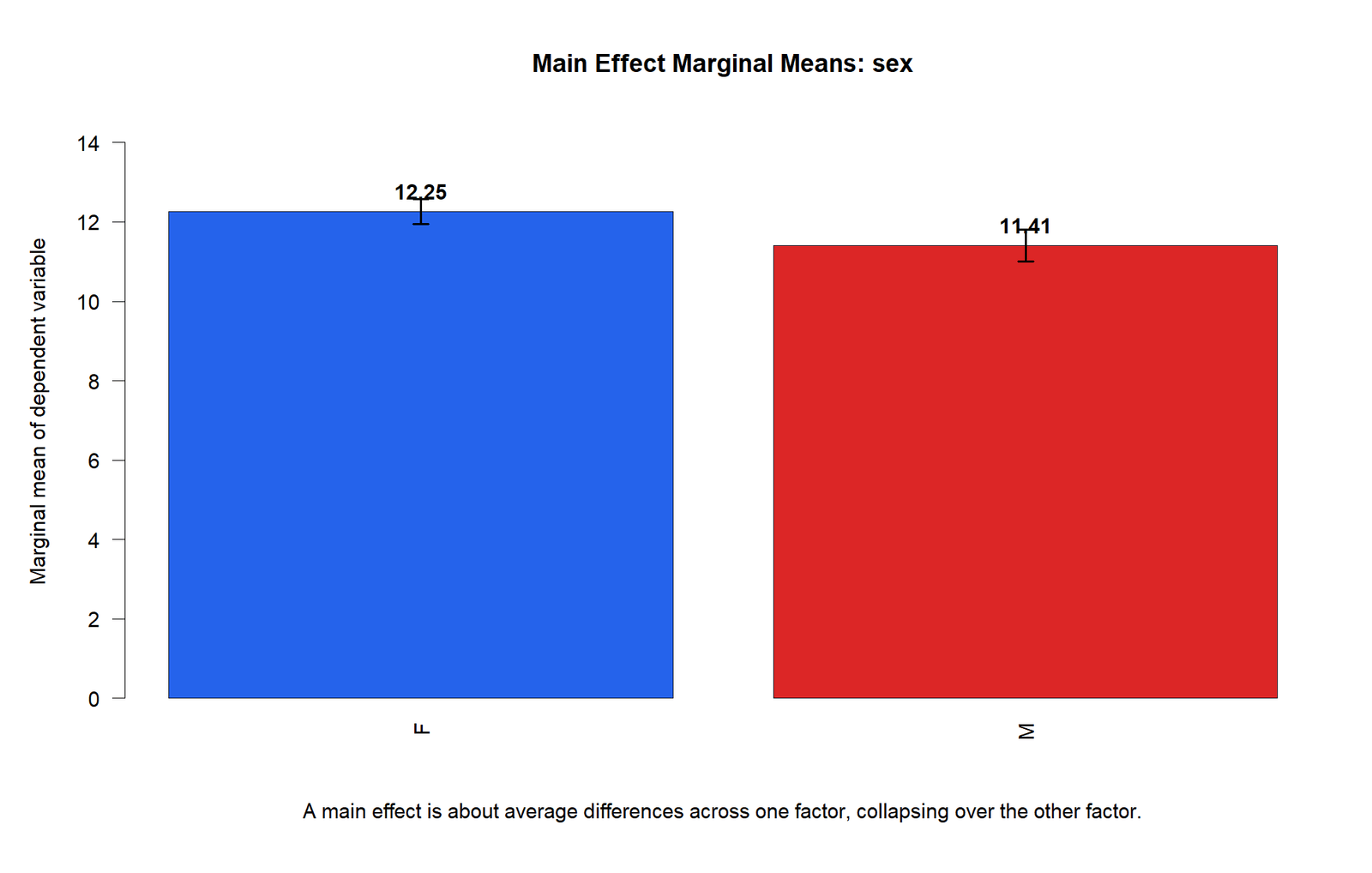
The R Factor A chart shows that female students have a higher average G3 than male students in the marginal summary. This is consistent with the SPSS Type-III direction of the sex effect.
Because the sex effect is smaller and method-sensitive, the article should report it carefully. The practical difference is not as central as the studytime difference.
R Chart 3: Main Effect Marginal Means for Factor B
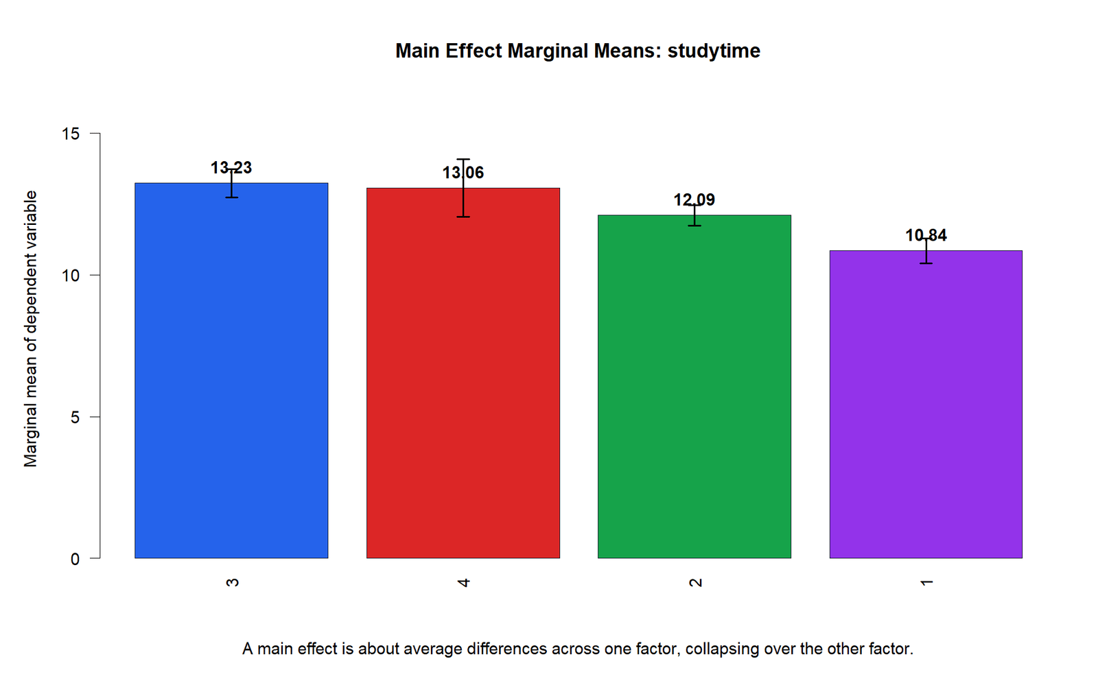
The R Factor B chart confirms the main studytime pattern. Mean G3 is lowest in the lowest studytime group and higher in groups 2, 3 and 4.
This chart validates the main conclusion that studytime is the clearest factor in the factorial ANOVA model.
R Chart 4: Interaction Profile Plot
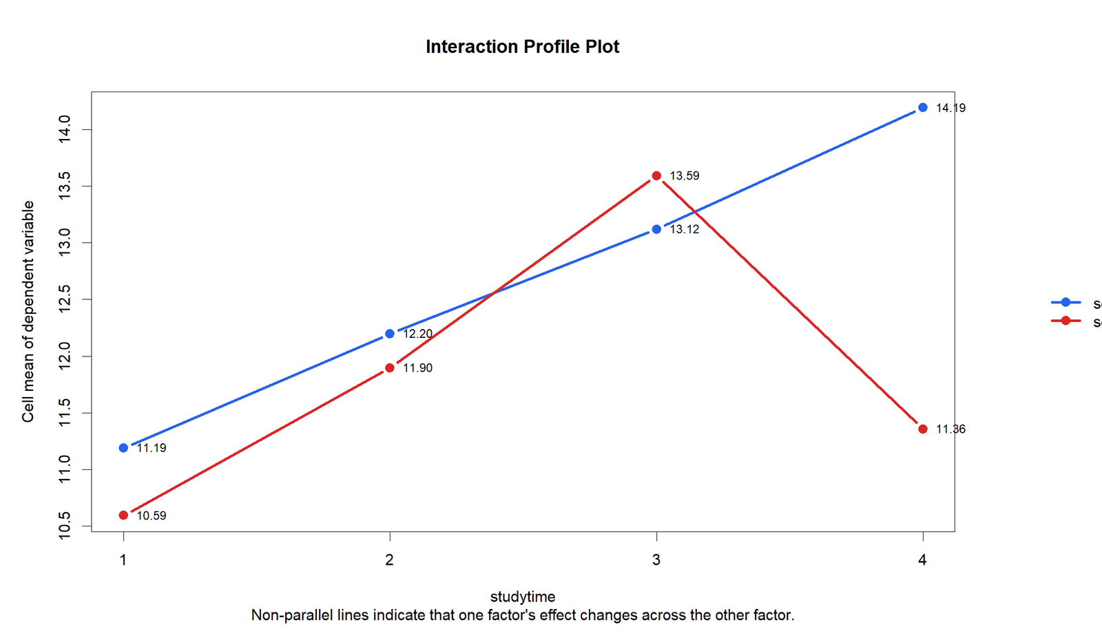
The R interaction profile plot confirms the same visual pattern as Python. The lines are not perfectly parallel, but the overall interaction test does not reach statistical significance.
This reinforces the correct reporting: mention the observed profile pattern, but do not claim a statistically significant interaction.
R Chart 5: Interaction Cell Mean Heatmap
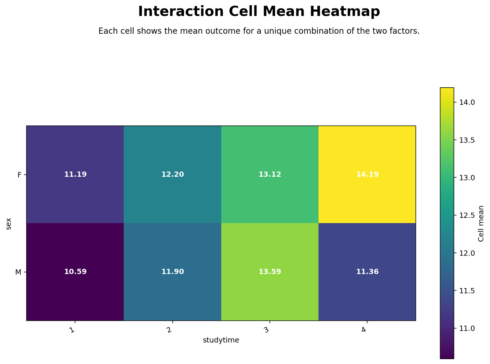
The R heatmap validates the cell mean pattern. The highest female studytime cell has a high mean, and the male high-studytime cell is lower than the female high-studytime cell.
This cell-level view helps explain why simple effects can appear interesting even when the overall interaction is not significant. It should be used as context, not as the main conclusion.
R Chart 6: Cell Size Balance Map
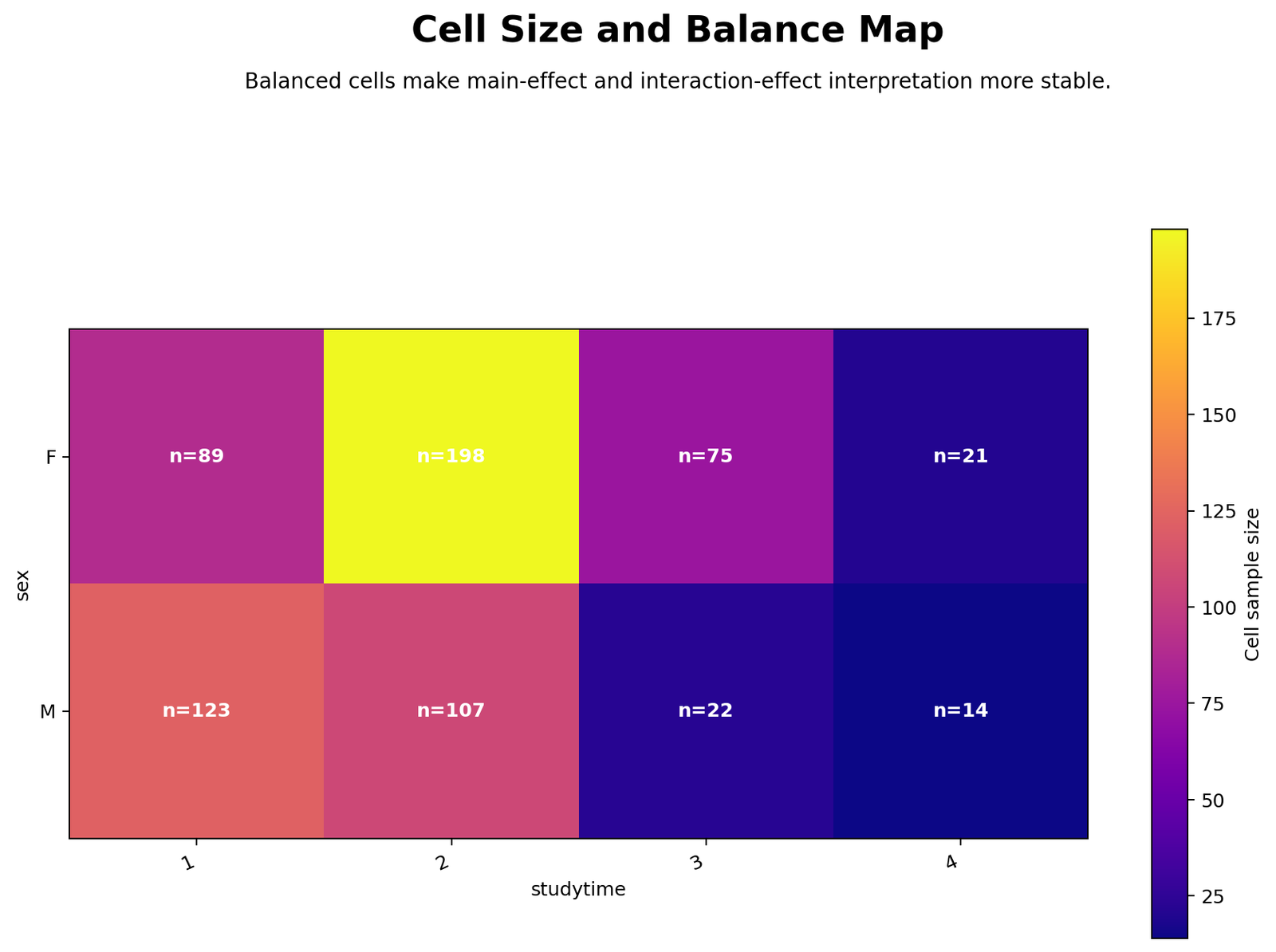
The R balance map confirms that the design is unbalanced. Some sex × studytime combinations have many cases, while others have small sample sizes.
This is important for interpretation because unbalanced designs make the choice of sums of squares more visible. It also warns against overinterpreting small cells.
R Chart 7: Simple Effects p-values
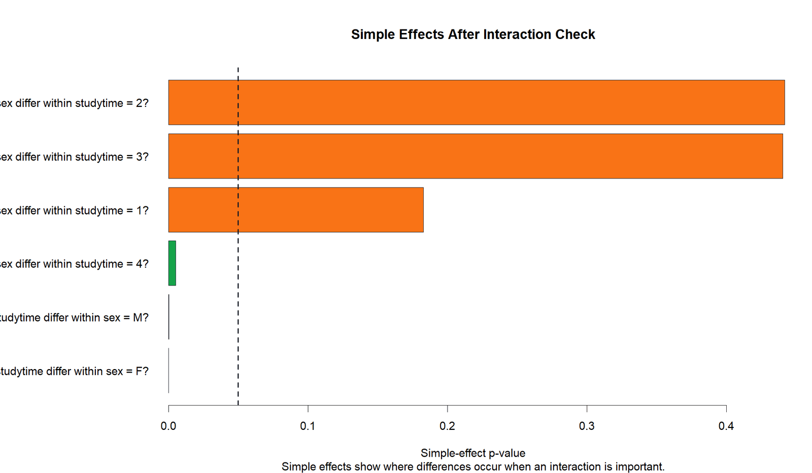
The R simple effects chart confirms that studytime differs within each sex group. It also confirms that sex differs clearly only within the highest studytime group.
Since the interaction is not significant, these simple effects should be interpreted as supporting or exploratory detail. The main report should stay focused on the main studytime effect.
R Chart 8: Effect Decomposition Sum of Squares
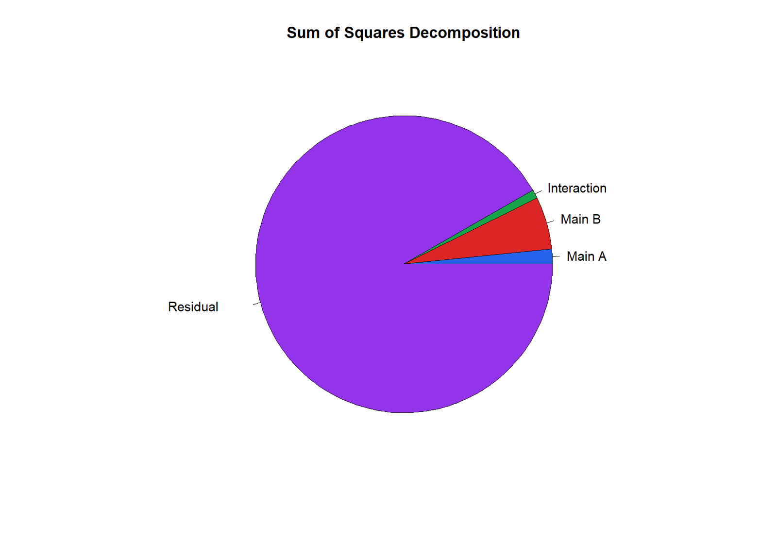
The R effect decomposition chart validates that studytime contributes more model variation than the interaction. The residual error remains large, which is normal in real student performance data.
This chart supports a practical interpretation. Statistical significance does not mean a factor explains all performance differences; it means the average group differences are unlikely to be due to random sampling alone.
R Chart 9: Distribution by Interaction Cell
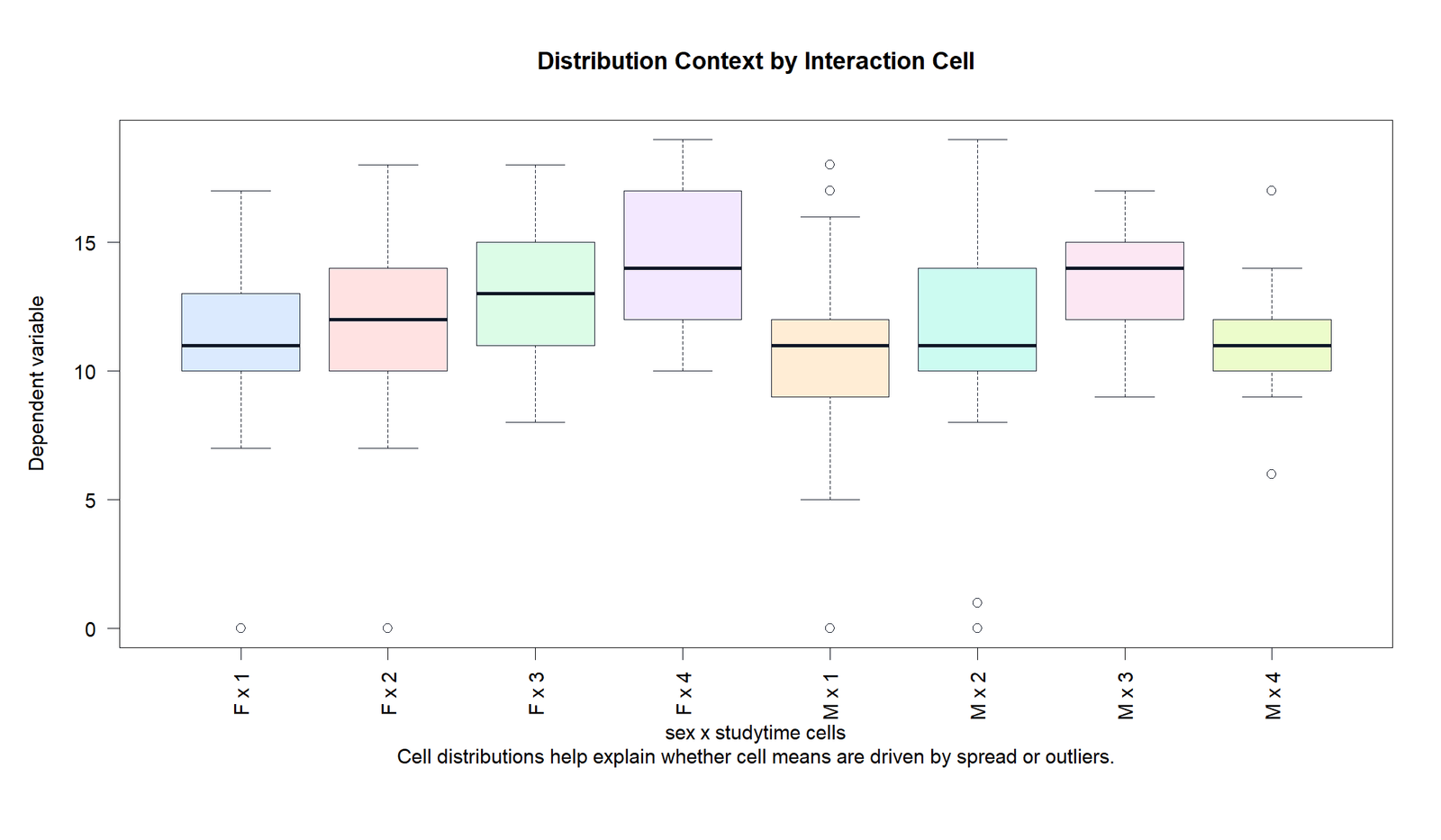
The R distribution chart confirms that the cell-level patterns include both mean differences and spread differences. Some cells are concentrated, while others include wider grade ranges.
This visual validation helps readers understand why factorial ANOVA should be interpreted with both tables and plots. Main effects, interactions, simple effects and distributions all answer different parts of the same question.
SPSS, R, Python and Excel Workflows for Main Effects vs Interaction Effects
The same factorial ANOVA workflow can be completed in SPSS, R, Python and Excel. SPSS gives a clear menu-based output for Type-III tests and profile plots. R and Python are better for reproducible reports and custom visualizations. Excel can run a two-factor ANOVA workflow, but it is less flexible for simple effects and publication-ready charts.
SPSS Workflow
| Step | SPSS Action | Purpose |
|---|---|---|
| Open data | File > Open > Data | Load the cleaned dataset containing G3, sex and studytime. |
| Run factorial ANOVA | Analyze > General Linear Model > Univariate | Set G3 as dependent variable and sex/studytime as fixed factors. |
| Add model terms | Full factorial model | Estimate sex, studytime and sex × studytime. |
| Request plots | Plots > studytime on horizontal axis and sex as separate lines | Create the interaction profile plot. |
| Request effect sizes | Options > Estimates of effect size | Report partial eta squared. |
| Interpret output | Check Levene test, Tests of Between-Subjects Effects and profile plot | Decide main effects and interaction effects. |
R Workflow
| Step | R Action | Purpose |
|---|---|---|
| Read data | read.csv() | Import the dataset. |
| Set factors | factor(sex) and factor(studytime) | Make sure variables are categorical. |
| Fit model | aov(G3 ~ sex * studytime) | Estimate main effects and the interaction. |
| Check results | summary(model) | Read F statistics and p-values. |
| Plot interaction | interaction.plot() or ggplot2 | Visualize whether lines are parallel or changing. |
Python Workflow
| Step | Python Action | Purpose |
|---|---|---|
| Read data | pandas.read_csv() | Load G3, sex and studytime variables. |
| Fit model | ols("G3 ~ C(sex) * C(studytime)") | Estimate the factorial ANOVA model. |
| ANOVA table | sm.stats.anova_lm() | Get sums of squares, F statistics and p-values. |
| Summarize cells | groupby(["sex","studytime"]) | Calculate cell means, standard errors and confidence intervals. |
| Plot results | matplotlib | Create marginal means, interaction plot and heatmap. |
Excel Workflow
Excel can run a two-factor ANOVA through the Analysis ToolPak when the data are arranged properly. Excel is helpful for learning the logic of main effects and interactions, but SPSS, R or Python is better for unbalanced designs, simple effects and advanced plots.
| Excel Item | Formula or Action | Purpose |
|---|---|---|
| Cell mean | =AVERAGEIFS(G3_range, sex_range, sex_level, studytime_range, studytime_level) | Calculate each sex × studytime mean. |
| Cell count | =COUNTIFS(sex_range, sex_level, studytime_range, studytime_level) | Check balance across cells. |
| Marginal mean | =AVERAGEIF(factor_range, factor_level, G3_range) | Calculate main-effect means. |
| Two-factor ANOVA | Data > Data Analysis > ANOVA: Two-Factor | Estimate main effects and interaction when the layout is suitable. |
| Profile plot | Line chart of cell means | Visualize interaction patterns. |
Code Blocks for Main Effects vs Interaction Effects
SPSS Syntax
UNIANOVA G3 BY sex studytime
  /METHOD = SSTYPE(3)
  /INTERCEPT = INCLUDE
  /PLOT = PROFILE(studytime*sex)
  /PRINT = DESCRIPTIVE ETASQ HOMOGENEITY
  /CRITERIA = ALPHA(.05)
  /DESIGN = sex studytime sex*studytime.
R Code
data <- read.csv("dataset.csv")

data$sex <- factor(data$sex)
data$studytime <- factor(data$studytime)

model <- aov(G3 ~ sex * studytime, data = data)
summary(model)

# Cell means

aggregate(G3 ~ sex + studytime, data = data, function(x) {
c(n = length(x), mean = mean(x), sd = sd(x))
})

# Interaction plot

interaction.plot(
x.factor = data$studytime,
trace.factor = data$sex,
response = data$G3,
fun = mean,
xlab = "Studytime",
ylab = "Mean G3",
trace.label = "Sex"
)
Python Code
import pandas as pd
import statsmodels.api as sm
import statsmodels.formula.api as smf

df = pd.read_csv("dataset.csv")

df["sex"] = df["sex"].astype("category")
df["studytime"] = df["studytime"].astype("category")

# Two-way / factorial ANOVA model

model = smf.ols("G3 ~ C(sex) * C(studytime)", data=df).fit()

# ANOVA table

anova_table = sm.stats.anova_lm(model, typ=2)
print(anova_table)

# Cell means

cell_summary = (
df.groupby(["sex", "studytime"])["G3"]
.agg(["count", "mean", "std"])
.reset_index()
)

print(cell_summary)

# Main effect marginal means

sex_means = df.groupby("sex")["G3"].agg(["count", "mean", "std"])
studytime_means = df.groupby("studytime")["G3"].agg(["count", "mean", "std"])

print(sex_means)
print(studytime_means)
Excel Formula Pattern
Cell Mean:
=AVERAGEIFS(G3_range, sex_range, "F", studytime_range, 1)

Cell Count:
=COUNTIFS(sex_range, "F", studytime_range, 1)

Main Effect Mean for Sex:
=AVERAGEIF(sex_range, "F", G3_range)

Main Effect Mean for Studytime:
=AVERAGEIF(studytime_range, 1, G3_range)

Interaction Plot:
Create a table of sex × studytime cell means.
Use studytime on the horizontal axis.
Use separate lines for female and male groups.

Interpretation:
Parallel lines = weak or no interaction.
Non-parallel or crossing lines = possible interaction.
APA Reporting Wording for Main Effects vs Interaction Effects
A two-way factorial ANOVA was conducted to examine the effects of sex and studytime on G3 final grade. The interaction between sex and studytime was not statistically significant, F(3, 641) = 2.233, p = .083, partial η² = .010, indicating that the studytime pattern did not differ significantly by sex at α = .05.
The main effect of studytime was statistically significant, F(3, 641) = 13.193, p < .001, partial η² = .058, showing that average G3 differed across studytime groups. The lowest studytime group had the lowest mean G3 score, while the higher studytime groups had higher means. The main effect of sex was small and should be reported with the selected sum-of-squares method; in the SPSS Type-III output, the sex effect was significant, F(1, 641) = 5.190, p = .023, partial η² = .008.
Short APA version: A two-way ANOVA showed a significant main effect of studytime on G3, F(3, 641) = 13.193, p < .001, partial η² = .058. The sex × studytime interaction was not significant, F(3, 641) = 2.233, p = .083, partial η² = .010. Therefore, the studytime main effect was interpreted directly.
Common Mistakes in Main Effects vs Interaction Effects
| Mistake | Why It Is a Problem | Better Practice |
|---|---|---|
| Interpreting main effects before checking interaction | A significant interaction can make average main effects misleading. | Check and report the interaction first. |
| Calling a visual crossing a significant interaction | A chart pattern still needs statistical support. | Use the interaction p-value and effect size. |
| Ignoring cell sizes | Small cells can make cell means unstable. | Report a balance map or cell-count table. |
| Forgetting sums-of-squares method | Unbalanced factorial ANOVA can give different main-effect p-values. | Report Type II or Type III clearly. |
| Overusing simple effects when interaction is not significant | Simple effects can distract from the main result. | Use simple effects mainly as context unless they were planned. |
Most important warning: Do not say the interaction is significant just because the profile plot is not perfectly parallel. In this example, the interaction p-value is about .083, so the correct α = .05 decision is not significant.
Downloads and Resources
Use the following downloadable outputs to verify the Main Effects vs Interaction Effects result and compare the SPSS, Python and R workflows.
SPSS Output PDF
Complete SPSS output with cell counts, descriptives, Levene test, factorial ANOVA, profile plots and simple effects.
Python Report PDF
Python verification report with ANOVA table, cell summaries, marginal means and simple effects.
R Report PDF
R validation report with factorial ANOVA results, cell summaries and supporting charts.
FAQs About Main Effects vs Interaction Effects
What is a main effect?
A main effect is the average effect of one factor on the dependent variable, ignoring or averaging over the levels of the other factor.
What is an interaction effect?
An interaction effect occurs when the effect of one factor depends on the level of another factor.
Which should be interpreted first, main effect or interaction effect?
The interaction effect should be checked first. If the interaction is significant, main effects may be misleading unless they are explained with the interaction pattern.
What was the interaction result in this example?
The sex × studytime interaction was not statistically significant at α = .05, with p around .083.
What was the strongest main effect in this example?
The studytime main effect was the clearest and most stable result. Average G3 scores differed across studytime groups.
Why can software give different main effect p-values?
In unbalanced factorial ANOVA, Type-II and Type-III sums of squares can produce different p-values for some main effects. The analyst should report the method used.
What is a profile plot?
A profile plot is an interaction plot that shows cell means across one factor with separate lines for another factor. Non-parallel lines suggest a possible interaction.
Can this analysis be done in Excel?
Yes, Excel can run a two-factor ANOVA through the Analysis ToolPak when the data are arranged correctly, but SPSS, R or Python is better for unbalanced designs and interaction plots.

