
Logistic Regression: Formula, Interpretation, SPSS, Python, R and Excel Guide
Logistic Regression estimates the probability of a binary event by modelling log odds as a function of predictors. This worked analysis uses 649 students, defines passing as G3 ≥ 10, explains coefficients and odds ratios, interprets eight diagnostic and performance charts, and compares SPSS, Python, R and Excel workflows.
549 events · 100 non-events
8 Python + 8 R charts
SPSS · Python · R · Excel
Model Overview
What this model is and when it is used: Logistic Regression is a generalized linear model for a binary dependent variable coded 0 and 1. It is used when the research question concerns the probability, odds or classification of an event such as pass versus fail, disease versus no disease, purchase versus no purchase, or default versus no default. Predictors may be continuous, ordinal, binary or categorical; categorical predictors are represented through reference-coded indicator variables. The model uses a logit link so an unrestricted linear predictor can be converted into a valid probability between 0 and 1. Coefficients describe adjusted changes in log odds, exponentiated coefficients are odds ratios, and fitted probabilities can be evaluated through discrimination, calibration and classification metrics.
Quick Answer
Model fit and prediction
The nine-predictor model estimates the probability that logit_pass = 1.
- McFadden pseudo-R²: 0.6853
- Sensitivity: 0.9672
- Specificity: 0.7600
- F1 score: 0.9620
Strongest adjusted predictors
Odds ratios express multiplicative changes in the adjusted odds of passing.
- G2: OR = 4.6486, p < .001
- G1: OR = 1.8542, p < .001
- age: OR = 1.5523, p = .0154
- school_MS: OR = 0.3863, p = .0289
Table of Contents
- Why this dataset needs Logistic Regression
- How Logistic Regression works
- Variables used
- Results at a glance
- Eight chart stories
- R charts with matching explanation boxes
- Complete coefficient tables
- Predicted probabilities and classification
- Diagnostics and model choice
- SPSS, Python, R and Excel
- Code
- Advanced interpretation
- APA-style reporting
- Publication checklist
- Downloads
- Related guides
- FAQs
Why This Dataset Needs Logistic Regression
Generalized Linear Model can generate predictions below zero or above one and assumes a constant residual variance. Logistic Regression instead uses a binomial variance and a logit link, producing fitted probabilities that remain inside the valid 0–1 range.
The event prevalence is high: 549 of 649 students pass. A majority-class rule predicting pass for everyone would already achieve 84.59% accuracy, so the fitted 93.53% accuracy must be evaluated with effect size, specificity, precision, calibration and ROC AUC. This Logistic Regression interpretation applies to the stated event coding and predictor adjustment.
What Is Logistic Regression?
Logistic Regression is a regression method for an outcome that represents two mutually exclusive states, such as pass versus not pass, disease versus no disease, purchase versus no purchase, or default versus no default. Instead of predicting an unrestricted continuous value, the model estimates the conditional probability that an observation belongs to the event category coded 1.
The central feature of the model is the logit link. A linear combination of predictors can take any real value, but a probability must remain between 0 and 1. the model solves this constraint by modeling the logarithm of the event odds. The inverse-logit transformation then converts the fitted log odds back into a valid probability. This Logistic Regression interpretation applies to the stated event coding and predictor adjustment.
In the the model formula, pᵢ is the probability that observation i has outcome 1, pᵢ/(1−pᵢ) is the event odds, β₀ is the intercept, β coefficients are adjusted log-odds effects, and X variables are the predictors. The right side is called the linear predictor or logit. This Logistic Regression interpretation applies to the stated event coding and predictor adjustment.
The second the model formula is the inverse logit. It turns ηᵢ into a probability. Very negative logits produce probabilities close to 0, a logit of 0 produces probability 0.50, and very positive logits produce probabilities close to 1. The characteristic S-shaped probability curve is a consequence of this transformation. This Logistic Regression interpretation applies to the stated event coding and predictor adjustment.
Why Logistic Regression Is Called Logistic
The word logistic refers to the logistic function used to transform an unrestricted linear predictor into a bounded probability. The logistic function rises smoothly from 0 to 1. the model therefore allows predictors to have additive effects on the log-odds scale while preserving a valid probability scale. This Logistic Regression interpretation applies to the stated event coding and predictor adjustment.
The word regression indicates that the model relates an outcome to one or more explanatory variables. Although the outcome is categorical, the method still estimates coefficients, tests hypotheses, constructs confidence intervals, calculates fitted values and evaluates residual information in a regression framework. This Logistic Regression interpretation applies to the stated event coding and predictor adjustment.
The Binary Outcome in This Analysis
The worked the model example creates logit_pass from final grade G3. A student is coded 1 when G3 is at least 10 and 0 when G3 is below 10. Among 649 students, 549 are events and 100 are non-events. The event prevalence is therefore 549/649 = 0.8459, or 84.59%. This Logistic Regression interpretation applies to the stated event coding and predictor adjustment.
the model treats the coding carefully because the model predicts the probability of the category coded 1. Reversing the coding would reverse coefficient signs and replace each odds ratio with its reciprocal. A clear outcome definition is therefore required before the model results are interpreted. This Logistic Regression interpretation applies to the stated event coding and predictor adjustment.
Probability, Odds and Log Odds
Probability, odds and log odds describe the same event on different scales. A probability of 0.50 corresponds to odds of 1, because the event and non-event are equally likely. A probability of 0.80 corresponds to odds of 4, because the event is four times as likely as the non-event. the model uses log odds because this scale can extend from negative infinity to positive infinity. This Logistic Regression interpretation applies to the stated event coding and predictor adjustment.
| Probability p | Odds p/(1−p) | Log Odds | Meaning |
|---|---|---|---|
| 0.10 | 0.111 | −2.197 | The event is much less likely than the non-event. |
| 0.25 | 0.333 | −1.099 | One event is expected for roughly three non-events. |
| 0.50 | 1.000 | 0.000 | Event and non-event are equally likely. |
| 0.75 | 3.000 | 1.099 | The event odds are three to one. |
| 0.90 | 9.000 | 2.197 | The event is much more likely than the non-event. |
What Logistic Regression Coefficients Estimate
A the model coefficient estimates the adjusted change in log odds associated with a one-unit predictor increase while the other model variables are held constant. The raw coefficient is mathematically useful but often difficult to communicate. Exponentiating the coefficient produces an odds ratio. This Logistic Regression interpretation applies to the stated event coding and predictor adjustment.
For G2, the the model coefficient is 1.5366. Its exponent is 4.6486. Holding G1, studytime, failures, absences, age, school, sex and address constant, one additional G2 point multiplies the odds of passing by approximately 4.65. This Logistic Regression interpretation applies to the stated event coding and predictor adjustment.
For school, the the model coefficient comparing MS with GP is −0.9511. The odds ratio is 0.3863. Under this nine-predictor model, the adjusted pass odds for MS students are approximately 61.37% lower than the odds for GP students because 1 − 0.3863 = 0.6137. This Logistic Regression interpretation applies to the stated event coding and predictor adjustment.
Adjusted Effects Rather Than Simple Group Comparisons
Every the model coefficient is conditional on the other variables in the equation. The G2 odds ratio is not the unadjusted relationship between G2 and passing. It is the relationship after G1, studytime, failures, absences, age, school, sex and address are controlled. This Logistic Regression interpretation applies to the stated event coding and predictor adjustment.
Conditional interpretation is important when predictors overlap. G1 and G2 measure related academic performance. the model assigns each coefficient the association that remains after accounting for the other grade and all additional covariates. A coefficient can therefore change when the predictor set changes. This Logistic Regression interpretation applies to the stated event coding and predictor adjustment.
Maximum-Likelihood Estimation
Ordinary least squares is not used to estimate the model because binary residuals do not satisfy the constant-variance Gaussian assumptions of linear regression. the model uses maximum likelihood. The fitted coefficients maximize the likelihood of observing the recorded pattern of 549 events and 100 non-events. This Logistic Regression interpretation applies to the stated event coding and predictor adjustment.
Software usually estimates the model through an iterative algorithm. Starting coefficient values generate fitted probabilities. The algorithm updates the coefficients, recalculates probabilities and continues until the log likelihood changes by less than a convergence tolerance. Convergence does not guarantee a good model, but non-convergence signals that the estimates should not be interpreted without investigation. This Logistic Regression interpretation applies to the stated event coding and predictor adjustment.
Logistic Regression as a Generalized Linear Model
the model is a binomial generalized linear model with a logit link. The random component is the Bernoulli or binomial outcome, the systematic component is the linear predictor, and the link component is the logit transformation. This structure connects the model to other generalized linear models such as Poisson and Gamma regression. This Logistic Regression interpretation applies to the stated event coding and predictor adjustment.
The binomial variance depends on the probability through p(1−p). Variability is largest near p = 0.50 and smaller near probabilities 0 or 1. the model therefore uses a family-specific variance rather than assuming one constant residual variance. This Logistic Regression interpretation applies to the stated event coding and predictor adjustment.
Prediction and Explanation
the model can support explanation, risk estimation, classification and prediction. For explanation, the emphasis is on coefficients, odds ratios, confidence intervals and theoretically meaningful covariate adjustment. For prediction, the emphasis shifts toward calibration, discrimination, validation, threshold selection and the consequences of false positive and false negative decisions. This Logistic Regression interpretation applies to the stated event coding and predictor adjustment.
A high the model AUC does not automatically imply accurate probabilities. A model may rank events above non-events very effectively while producing probabilities that are systematically too high or too low. Conversely, a calibrated the model model can have limited discrimination if most observations receive similar risks. This Logistic Regression interpretation applies to the stated event coding and predictor adjustment.
Discrimination in Logistic Regression
Discrimination describes how well the model separates observations with outcome 1 from observations with outcome 0. The ROC curve evaluates sensitivity and false-positive rate across all possible probability cutoffs. The area under the ROC curve is 0.9768, indicating excellent separation in the analyzed data. This Logistic Regression interpretation applies to the stated event coding and predictor adjustment.
An AUC of 0.9768 can be interpreted as the probability that a randomly selected passing student receives a higher fitted probability than a randomly selected non-passing student, subject to the usual assumptions and tie handling. the model discrimination should still be validated on new observations because in-sample AUC can be optimistic. This Logistic Regression interpretation applies to the stated event coding and predictor adjustment.
Classification in Logistic Regression
Classification converts the model probabilities into predicted categories by choosing a cutoff. At the 0.50 cutoff, probabilities of at least 0.50 are classified as pass. The model correctly classifies 76 non-events and 531 events, while 24 non-events are false positives and 18 events are false negatives. This Logistic Regression interpretation applies to the stated event coding and predictor adjustment.
The the model accuracy is 607/649 = 93.53%. Sensitivity is 531/549 = 96.72%, and specificity is 76/100 = 76.00%. Because the event class is common, accuracy should be interpreted with sensitivity, specificity, precision, F1 score and the baseline event rate. This Logistic Regression interpretation applies to the stated event coding and predictor adjustment.
Calibration in Logistic Regression
Calibration asks whether the model probabilities agree with observed event frequencies. A group of students assigned an average probability of 0.70 should have an observed pass rate close to 70%. The calibration-by-decile chart shows close agreement across most probability groups. This Logistic Regression interpretation applies to the stated event coding and predictor adjustment.
Calibration can be assessed visually, with calibration intercept and slope, with grouped tests and with prediction-error measures. A grouped goodness-of-fit test can be sensitive to sample size and grouping decisions. the model calibration should therefore not be reduced to one p-value.
Common Forms of Logistic Regression
| Method | Outcome Structure | Main Interpretation |
|---|---|---|
| Binary Logistic Regression | Two unordered categories | Event probability and odds ratio. |
| Multinomial Logistic Regression | Three or more unordered categories | Category odds relative to a reference category. |
| Ordinal Logistic Regression | Ordered categories | Cumulative odds under a proportional-odds or alternative structure. |
| Conditional Logistic Regression | Matched sets or strata | Within-stratum odds ratios. |
| Mixed-Effects Logistic Regression | Clustered binary observations | Conditional effects with random intercepts or slopes. |
| GEE Logistic Regression | Correlated binary observations | Population-average effects with robust covariance. |
| Penalized Logistic Regression | Many or correlated predictors | Shrunken coefficients for prediction and stability. |
When Standard Logistic Regression Is Not Enough
Standard the model assumes independent observations after conditioning on the predictors. Repeated measurements from one student, pupils nested within classrooms, or family members within households violate this independence structure. A generalized estimating equation or mixed-effects the model model may then be required.
Standard the model also assumes linearity between each continuous predictor and the logit. If the effect of age or G1 bends across its range, a single coefficient may be inadequate. Polynomial terms, restricted cubic splines or a generalized additive model can represent nonlinear logit relationships.
Complete separation occurs when a predictor or predictor combination perfectly distinguishes the outcome categories. Under complete separation, ordinary maximum-likelihood the model coefficients may diverge. Penalization, exact methods, bias-reduced estimation or a revised predictor structure may be needed.
What Logistic Regression Does Not Prove
the model estimates adjusted associations unless the study design and causal assumptions justify stronger conclusions. A significant odds ratio does not prove that changing the predictor will cause the event probability to change. Confounding, measurement error, selection mechanisms and model specification remain important.
In this student dataset, G1 and G2 are strong predictors of passing, but the model should be described as estimating conditional associations and probabilities. Causal language would require a design that supports intervention-based interpretation.
Applied Meaning of the Current Logistic Regression
The current the model model combines six numeric predictors and three categorical predictors. G2 has the largest positive adjusted odds ratio. G1 and age also increase adjusted pass odds, while the MS-versus-GP school contrast decreases adjusted pass odds in the nine-predictor specification.
Studytime, failures, absences, sex and address are not statistically significant at α = .05 after the other predictors are controlled. This does not prove that their effects are exactly zero. Their confidence intervals describe the range of values compatible with the fitted the model model and sampling uncertainty.
Core definition: the model models the log odds of a binary event as a linear function of predictors and transforms the fitted log odds into probabilities between 0 and 1.
Essential distinction: the model predicts a categorical event probability. It should not be confused with ordinary linear regression, which predicts an unbounded continuous mean.
For broader model selection, compare this method with the Generalized Linear Model and Binary Logistic Regression guides.
How Logistic Regression Works
Combine predictors into η = Xβ.
Use p = 1 / [1 + exp(−η)].
Report odds ratios, probabilities and threshold metrics.
The fitted Logistic Regression linear predictor η combines the intercept and nine predictor effects. GP school, female sex and rural address are the reference categories for the displayed categorical contrasts.
The inverse-logit equation converts the fitted the model logit into the probability of logit_pass = 1. Because the exponential function is always positive, the resulting probability always lies between 0 and 1.
Odds Form
The exponential of the the model linear predictor is the fitted event odds. Increasing predictor X by one unit multiplies these odds by exp(β), provided the remaining variables are unchanged.
Likelihood Function
The the model likelihood multiplies each observation’s probability contribution. For an event, the contribution is pᵢ; for a non-event, it is 1−pᵢ. Maximum likelihood chooses coefficients that maximize the complete product or, equivalently, the summed log likelihood.
Exact Fitted Equation
Using the Python/R coefficients, the fitted the model logit is approximately:
This the model equation should be used with the exact coding shown in the data dictionary. A categorical coefficient cannot be interpreted correctly without knowing its reference category.
Binary Random Component
The Logistic Regression outcome follows a Bernoulli structure for individual rows. Its conditional variance is p(1−p), so the variance changes with the fitted probability.
Systematic Component
The the model systematic component contains G1, G2, studytime, failures, absences, age, schoolMS, sexM and addressU. The intercept represents the log odds when numeric predictors equal zero and categorical predictors are at their references, which may not be a substantively realistic student profile.
binary Logistic Regression
The the model logit link makes predictor effects additive on the log-odds scale. The inverse link produces fitted passing probabilities.
Maximum Likelihood
The the model coefficients are maximum-likelihood estimates. Standard errors derive from the estimated information matrix under the fitted model.
Wald Tests
Each the model z statistic divides B by its standard error. The squared z statistic corresponds to a one-degree-of-freedom Wald chi-square test.
Likelihood-Ratio Tests
Nested the model models can be compared through their deviance difference. Likelihood-ratio tests are often preferred for joint terms or factors because they evaluate the change in overall likelihood.
Variables Used and Coding
| Variable | Definition and Coding | Role | Interpretation |
|---|---|---|---|
| logit_pass | 1 when G3 ≥ 10; 0 when G3 < 10. | Binary outcome | The model estimates probability of passing. |
| G3 | Final grade, used to create logit_pass. | Outcome source | Not entered as a predictor. |
| G1 | First-period grade. | Numeric predictor | One-point odds-ratio effect. |
| G2 | Second-period grade. | Numeric predictor | One-point odds-ratio effect. |
| studytime | Weekly study-time category. | Numeric/ordinal predictor | One-category increase. |
| failures | Number of prior class failures. | Numeric predictor | One additional failure. |
| absences | School absences. | Numeric predictor | One additional absence. |
| age | Student age in years. | Numeric predictor | One-year increase. |
| school | GP reference; MS comparison. | Categorical predictor | MS-versus-GP adjusted odds ratio. |
| sex | Female reference; male comparison. | Categorical predictor | Male-versus-female adjusted odds ratio. |
| address | Rural reference; urban comparison. | Categorical predictor | Urban-versus-rural adjusted odds ratio. |
Outcome Distribution
The Logistic Regression event category contains 549 students and the non-event category contains 100. The unequal class sizes affect baseline accuracy, precision and the practical consequences of threshold selection.
binary Logistic Regression
The the model categorical estimates depend on the chosen references. Changing the reference changes the sign and reciprocal odds ratio but does not change fitted probabilities or overall model likelihood.
Results at a Glance
Null log likelihood = −278.8928
AIC = 195.5231
Large likelihood improvement
Excellent discrimination
Accuracy = 93.53%
Nagelkerke R² = .783
Download the PDF Outputs
Open the full software reports for model tables, diagnostics and chart output.
Model fit in Logistic Regression is likelihood-based. The fitted log likelihood is −87.7616, compared with null log likelihood −278.8928. The large improvement indicates that the predictors explain substantial information about the binary outcome.
| Statistic | Value | Interpretation |
|---|---|---|
| N | 649 | All students enter the model. |
| Events / non-events | 549 / 100 | Passing is the majority event. |
| Log likelihood | −87.7616 | Higher values, closer to zero, indicate better likelihood fit for comparable models. |
| Residual deviance | 175.5231 | Twice the negative fitted log likelihood for this binomial model. |
| AIC | 195.5231 | Balances likelihood fit and parameter count for same-outcome model comparison. |
| McFadden pseudo-R² | 0.6853 | Large proportional improvement in log likelihood relative to the intercept-only model. |
| ROC AUC | 0.9768 | Excellent ranking discrimination. |
Deviance
the model deviance compares the fitted model with a saturated model. Deviance differences can test nested models. A smaller deviance indicates better fit when models analyze the same outcome and observations.
AIC
the model AIC is useful only for models fitted to the same response and data. It should not be compared across unrelated outcomes. A lower AIC is preferred when the likelihood conventions are comparable.
Pseudo R-Squared
McFadden pseudo-R² is not the proportion of outcome variance explained. the model pseudo-R² measures likelihood improvement relative to a null model. It must not be interpreted as ordinary linear-regression R².
Model-Fit Summary
| Measure | Python Result |
|---|---|
| N | 649 |
| Events / non-events | 549 / 100 |
| Event rate | 0.8459 |
| Log likelihood | −87.7616 |
| Null log likelihood | −278.8928 |
| Residual deviance | 175.5231 |
| AIC | 195.5231 |
| McFadden pseudo-R² | 0.6853 |
| ROC AUC | 0.9768 |
| Accuracy | 0.9353 |
| Precision | 0.9568 |
| Sensitivity | 0.9672 |
| Specificity | 0.7600 |
| F1 score | 0.9620 |
Coefficient Results
Python Logistic Regression identifies significant adjusted effects for schoolMS, G1, G2 and age. G2 has the strongest positive effect. The coefficients for sexM, addressU, studytime, failures and absences are not statistically significant at α = .05.
Python the model conclusion: the nine-predictor model has excellent discrimination and high event sensitivity. The model is less successful at identifying non-events than events, as shown by specificity of 0.7600 compared with sensitivity of 0.9672.
Eight Chart Stories: What Each Figure Actually Means
Each figure is interpreted in four steps: what it shows, exact values, statistical meaning and the next diagnostic action. This keeps the charts central to the analysis rather than treating them as decoration.
Chart 1: Binary Outcome Distribution
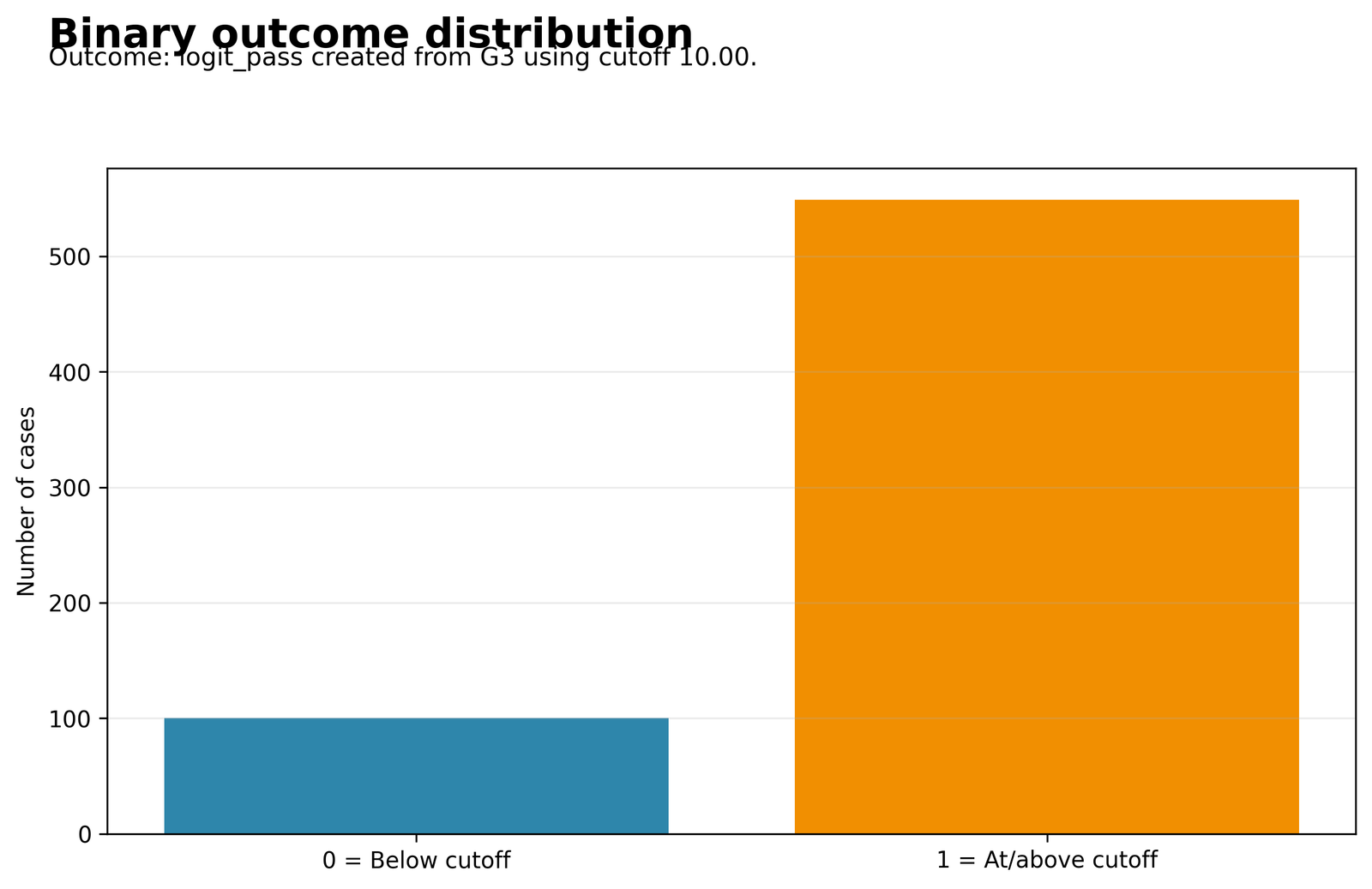
The bar chart establishes the class balance that affects every classification metric.
100 non-events and 549 events are observed. The event rate is 84.59%.
Most students in the dataset pass, while the non-passing group is much smaller. This means the model has abundant examples of passing students but only 100 examples from which to learn the pattern of non-passing students. The real modelling challenge is therefore not identifying the common passing group; it is correctly finding the smaller group that does not pass.
Do not describe the model as successful simply because overall accuracy is high. Judge whether it identifies the 100 non-passing students well enough for the intended educational decision, and give particular attention to specificity and false positives.
Chart 2: Predicted Probability Distribution
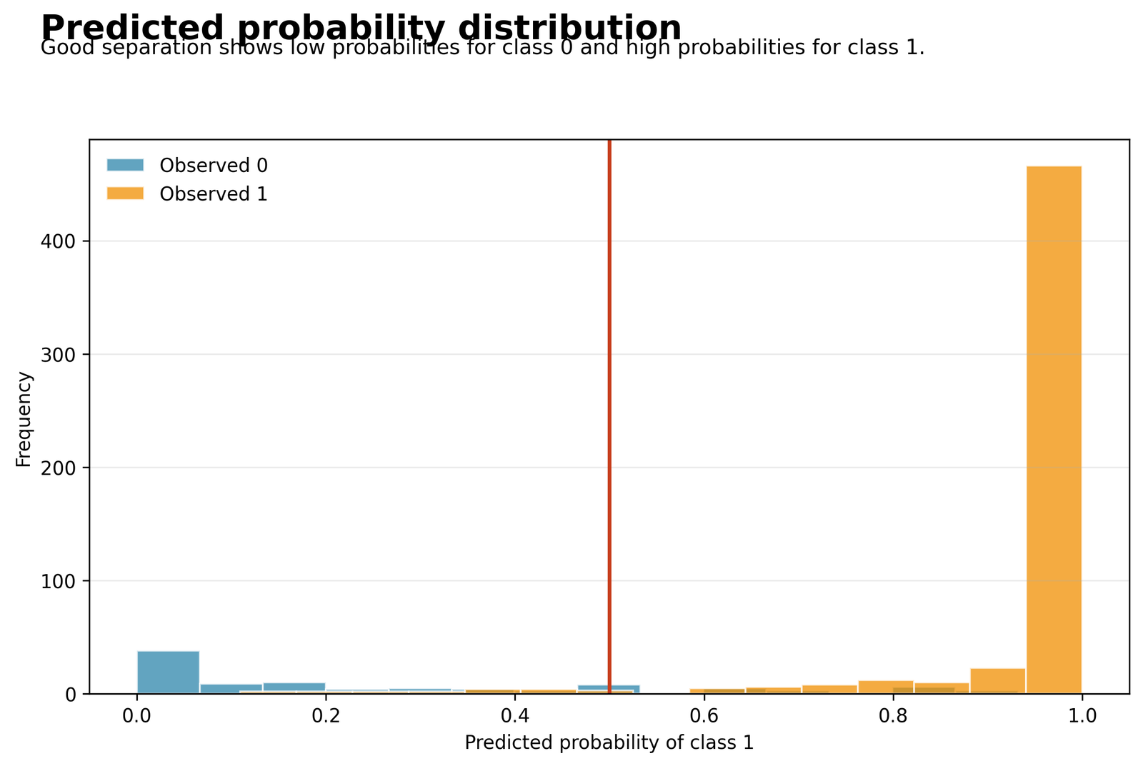
The histogram shows how fitted probabilities separate the observed outcome groups.
Most events receive probabilities near 0.90–1.00, while many non-events receive probabilities near 0.00–0.10. The cutoff is 0.50.
The model gives very high passing probabilities to most students who actually pass and very low probabilities to many students who do not pass. The errors occur mainly among borderline students whose academic profiles place them near the 0.50 decision boundary. These are the cases where the available predictors do not clearly separate pass from non-pass.
Students with probabilities near 0.50 should be treated as uncertain cases rather than confident classifications. Review their predictor profiles, consider additional relevant variables, and choose a cutoff that matches the cost of the two kinds of classification error.
Chart 3: binary Logistic Regression Curve
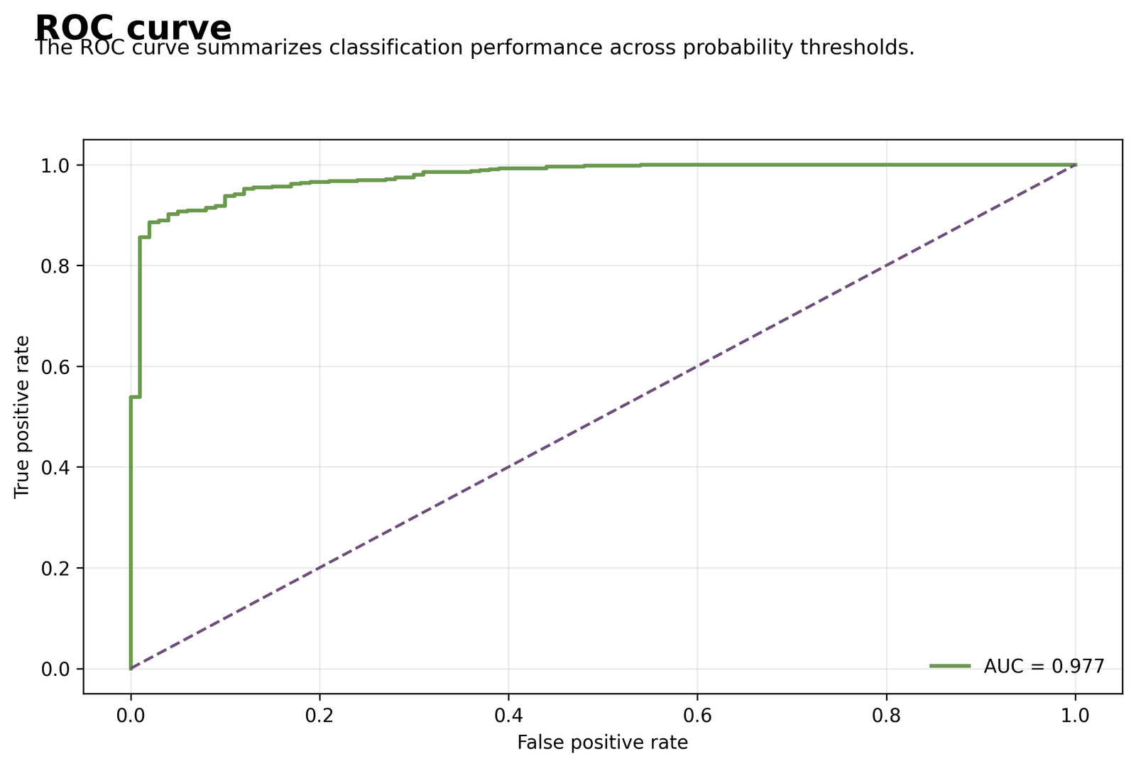
The curve evaluates sensitivity and false-positive rate across all possible thresholds.
The area under the curve is 0.9768, far above the random-ranking reference of 0.50.
Across almost every possible cutoff, the model keeps most passing students correctly identified while allowing comparatively few non-passing students to be incorrectly labelled as passing. In practical terms, students who pass are almost always ranked above students who do not pass, even before a single classification threshold is chosen.
The model is highly effective for ranking students by passing likelihood. Use the ROC result to support discrimination, but do not use it as proof that the numerical probabilities are accurate; probability Generalized Linear Model must be checked separately.
Chart 4: Confusion Matrix
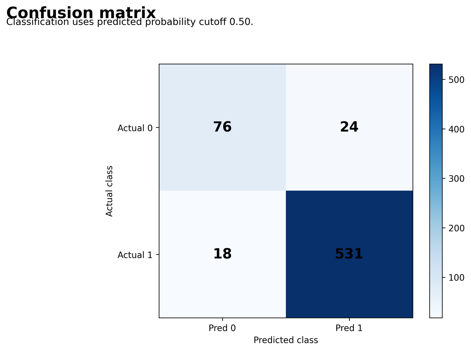
The matrix displays the exact event and non-event classification counts.
76 true negatives, 24 false positives, 18 false negatives and 531 true positives are observed.
The model correctly recognises 531 of the 549 passing students and incorrectly labels 18 passing students as non-passing. Among the 100 non-passing students, it correctly identifies 76 but labels 24 as passing. The larger practical weakness is therefore the failure to detect about one quarter of the non-passing group, not the detection of passing students.
When missing a non-passing student is costly, raise the probability cutoff or choose a threshold that improves specificity. When falsely flagging a passing student is more harmful, retain or lower the cutoff. Report the actual 76, 24, 18 and 531 counts with the selected decision rule.
Chart 5: Odds Ratios and Confidence Intervals
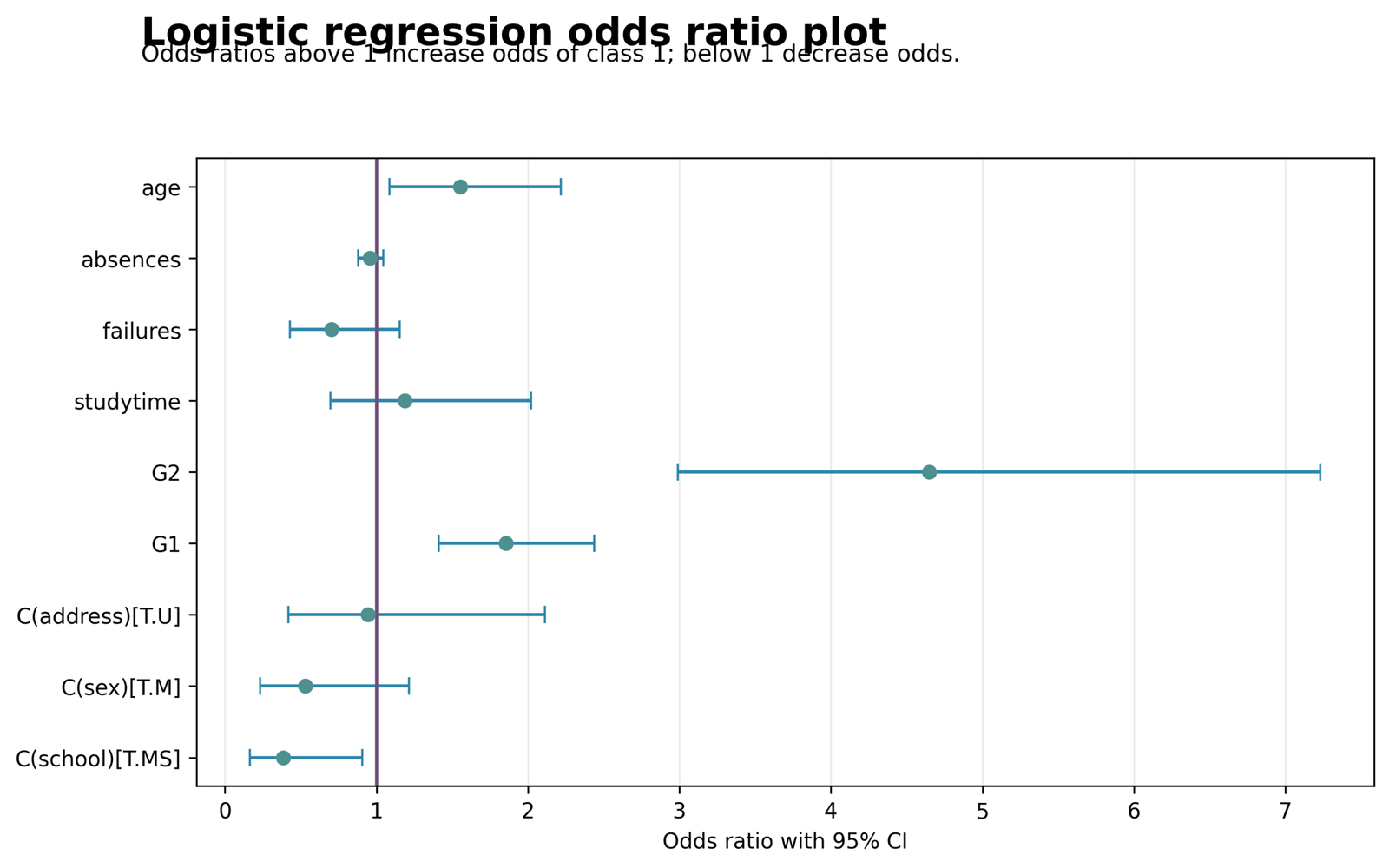
The forest plot converts log-odds coefficients into multiplicative adjusted effects.
G2 OR = 4.6486, G1 OR = 1.8542, age OR = 1.5523, and school_MS OR = 0.3863.
Recent academic performance drives most of the difference in passing likelihood. A one-point rise in G2 is associated with a very large increase in adjusted passing odds, while G1 also contributes positively. Older students have higher adjusted odds in this fitted sample, whereas students at MS have lower adjusted odds than comparable GP students after the other predictors are controlled.
The model indicates where the strongest adjusted associations lie: G2 first, then G1, age and school. These are not causal effects. Convert meaningful predictor changes into fitted probabilities for realistic student profiles before making educational interpretations.
Chart 6: Calibration by Probability Decile
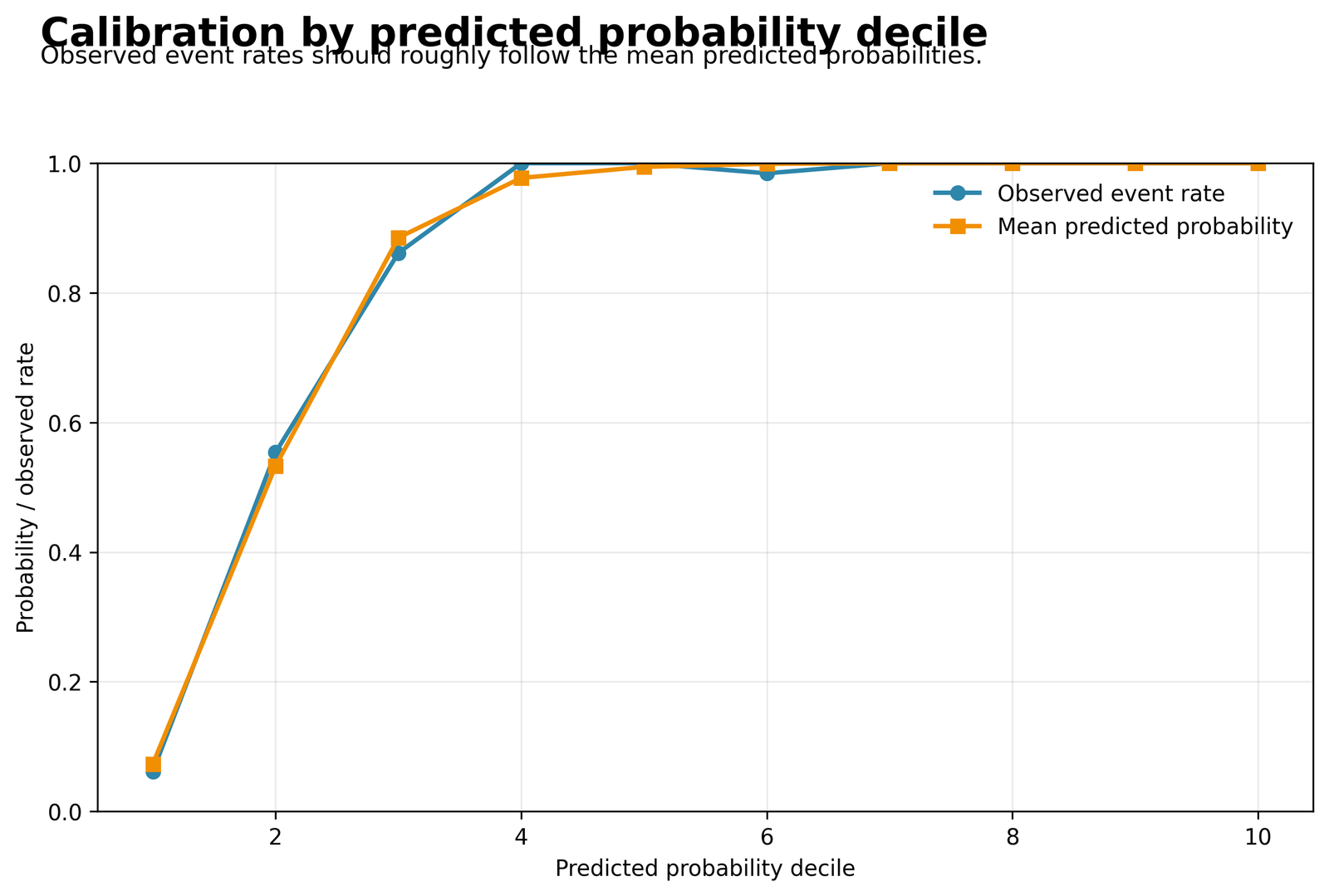
The chart compares numerical probability predictions with observed event frequencies.
Early groups are approximately 0.06 observed vs 0.07 predicted, 0.55 vs 0.53, and 0.86 vs 0.88.
Groups assigned low probabilities actually pass infrequently, groups assigned middle probabilities pass at roughly the predicted rate, and groups assigned high probabilities almost always pass. The model is therefore not only ranking students correctly; within this sample, its probability numbers broadly correspond to what happens in the observed data.
The probabilities are suitable for interpretation within the estimation sample, but they may become too high or too low in another school or cohort. Validate the calibration intercept and slope before using the probabilities for counselling, intervention or resource allocation.
Chart 7: Probability Across G1
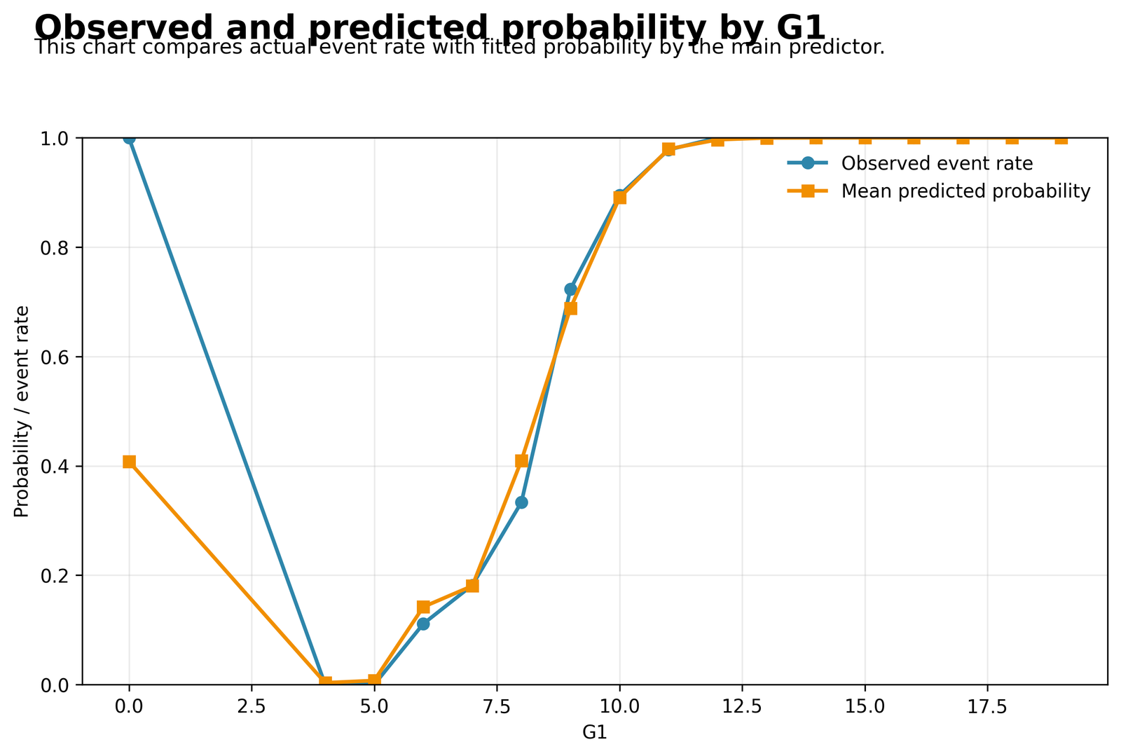
The grouped plot compares observed event rates with mean fitted probabilities at each G1 value.
At G1 = 8, observed and predicted probabilities are about 0.33 and 0.41; at G1 = 9, about 0.72 and 0.69; and at G1 = 10, both are near 0.90.
Passing likelihood changes most rapidly across the middle G1 range. Students around G1 = 8 have a substantial risk of not passing, while students around G1 = 10 are already very likely to pass. The chart shows a steep transition rather than a constant probability increase across all grade values.
The G1 range around 8–10 is the most informative zone for identifying borderline students. Sparse extreme values should not be overinterpreted, and the logit-linearity assumption should be checked with a flexible curve or spline.
Chart 8: Classification Performance Summary

The bar chart places four major performance measures on the same 0–1 scale.
AUC = 0.9768, accuracy = 0.9353, sensitivity = 0.9672, and specificity = 0.7600.
The model performs extremely well at ranking students and identifying the common passing group, but its ability to identify non-passing students is noticeably weaker. It misses only 18 of 549 passing students, yet it incorrectly classifies 24 of the 100 non-passing students as passing.
The model is strong for general screening, but a decision process focused on preventing unnoticed failure should place more weight on specificity than on overall accuracy. Threshold selection should be based on the real consequences of missing a non-passing student.
R Charts: Two Charts Followed by Two Matching Explanation Boxes
Each group first displays two R charts side by side. Directly underneath, two explanation boxes appear in the same left-to-right order, so each explanation aligns with the chart immediately above it.
R Chart 1: Binary Outcome Distribution
Passing is the normal outcome in this sample, while non-passing is comparatively uncommon. The model consequently has a much easier task recognising the majority passing group than learning the smaller non-passing pattern.
R Chart 2: Predicted Probability Distribution
Most passing students receive probabilities close to one and many non-passing students receive probabilities close to zero. The uncertain cases lie in the overlapping middle region, where the student profiles do not point clearly to one outcome.
R Chart 3: ROC Curve
The model preserves strong separation across many cutoffs: passing students are usually placed above non-passing students in the risk ranking.
R Chart 4: Confusion Matrix
Only 18 passing students are missed, but 24 of the 100 non-passing students are incorrectly labelled as passing. The model is therefore stronger at confirming passing than at detecting non-passing.
R Chart 5: Odds Ratios
G2 is the dominant adjusted predictor of passing, G1 contributes additional academic information, and the school contrast remains after the other variables are controlled. The chart shows which relationships remain after adjustment, not simple raw group differences.
R Chart 6: Calibration by Decile
Students assigned low, middle and high probabilities pass at rates close to those predicted. Within the analysed sample, the probability scale therefore corresponds reasonably well to the observed outcomes.
R Chart 7: Probability Across G1
Passing probability rises sharply between G1 values of about 8 and 10. This is the transition zone where small differences in prior grade correspond to large differences in expected passing probability.
R Chart 8: Performance Summary
The model is excellent at ranking and identifying passing students, but its weaker specificity shows that the smaller non-passing group remains more difficult to detect.
Complete Coefficient Results
The binary Logistic Regression in Logistic Regression is exp(B). Odds ratios above 1 indicate higher adjusted event odds, odds ratios below 1 indicate lower adjusted event odds, and an odds ratio of 1 indicates no change.
| Predictor | B | SE | p | Odds Ratio | 95% CI for OR | Decision |
|---|---|---|---|---|---|---|
| school: MS vs GP | −0.9511 | 0.4352 | .0289 | 0.3863 | [0.1646, 0.9066] | Significant |
| sex: M vs F | −0.6326 | 0.4226 | .1344 | 0.5312 | [0.2320, 1.2161] | Not significant |
| address: U vs R | −0.0595 | 0.4118 | .8851 | 0.9422 | [0.4203, 2.1121] | Not significant |
| G1 | 0.6174 | 0.1397 | <.001 | 1.8542 | [1.4101, 2.4380] | Significant |
| G2 | 1.5366 | 0.2254 | <.001 | 4.6486 | [2.9884, 7.2311] | Significant |
| studytime | 0.1719 | 0.2715 | .5266 | 1.1876 | [0.6976, 2.0218] | Not significant |
| failures | −0.3514 | 0.2518 | .1629 | 0.7037 | [0.4296, 1.1528] | Not significant |
| absences | −0.0433 | 0.0443 | .3283 | 0.9576 | [0.8780, 1.0445] | Not significant |
| age | 0.4397 | 0.1815 | .0154 | 1.5523 | [1.0875, 2.2157] | Significant |
Percentage Change in Odds
For an odds ratio above 1, the percentage increase is (OR−1)×100. The G1 odds ratio represents an 85.42% increase in adjusted passing odds per point. The G2 odds ratio represents a 364.86% increase per point.
For an odds ratio below 1, the percentage decrease is (1−OR)×100. The schoolMS odds ratio represents approximately a 61.37% decrease in adjusted passing odds relative to GP in the main the model model.
Confidence-Interval Rule
A 95% odds-ratio interval that excludes 1 corresponds to a two-sided coefficient test below approximately .05. the model intervals are preferred to a p-value alone because they show effect direction and uncertainty.
A raw Logistic Regression coefficient is a change in log odds. A positive coefficient raises the adjusted event odds, a negative coefficient lowers them, and a coefficient of zero leaves the adjusted odds unchanged.
| Term | B | Meaning on Log-Odds Scale |
|---|---|---|
| G1 | 0.6174 | Each one-point increase raises adjusted log odds by 0.6174. |
| G2 | 1.5366 | Each one-point increase raises adjusted log odds by 1.5366. |
| age | 0.4397 | Each additional year raises adjusted log odds by 0.4397. |
| schoolMS | −0.9511 | MS has lower adjusted log odds than reference school GP. |
Continuous Predictors
For a continuous predictor, the model assumes one constant coefficient on the logit scale unless nonlinear terms are added. The effect on probability is not constant: the same logit increase causes a larger probability change near p = 0.50 than near p = 0.01 or p = 0.99.
Categorical Predictors
For a dummy variable, the model compares the coded category with the reference category. The schoolMS coefficient compares MS with GP. The sexM coefficient compares male with female. The addressU coefficient compares urban with rural.
Statistical Significance
A the model Wald z test evaluates H₀: β = 0. G1, G2, age and school are significant in the nine-predictor model. Studytime, failures, absences, sex and address have p-values above .05.
Practical Significance
Statistical significance does not automatically establish practical importance. the model interpretation should consider the odds ratio, confidence interval, baseline probability, realistic predictor change and predicted probability difference.
Predicted Probabilities and Practical binary Logistic Regression
What the probability contributes
- A fitted value between 0 and 1.
- A continuous measure of event risk.
- A basis for calibration and decision analysis.
What the cutoff contributes
- A predicted class of 0 or 1.
- Cutoff-dependent sensitivity and specificity.
- Decision consequences through false positives and false negatives.
Classification is a secondary step applied to Logistic Regression probabilities. The probability model exists independently of the cutoff. Changing the cutoff changes predicted classes but not the fitted coefficients or probabilities.
| Metric | Formula | Result | Interpretation |
|---|---|---|---|
| Accuracy | (TP+TN)/N | 0.9353 | 93.53% of all cases are classified correctly. |
| Sensitivity | TP/(TP+FN) | 0.9672 | 96.72% of passing students are detected. |
| Specificity | TN/(TN+FP) | 0.7600 | 76.00% of non-passing students are detected. |
| Precision | TP/(TP+FP) | 0.9568 | 95.68% of predicted passes are actual passes. |
| F1 score | 2×precision×recall/(precision+recall) | 0.9620 | Harmonic balance of precision and sensitivity. |
| False-positive rate | FP/(FP+TN) | 0.2400 | 24.00% of non-events are classified as events. |
| False-negative rate | FN/(FN+TP) | 0.0328 | 3.28% of events are classified as non-events. |
Class Imbalance
Because the model analyzes an 84.59% event rate, accuracy is influenced by the majority class. Specificity is especially important because a model can achieve high accuracy while performing poorly on the smaller non-event class.
Decision Costs
The best the model threshold depends on whether false positives or false negatives are more costly. Educational screening may prioritize sensitivity, while resource allocation may require higher specificity.
The default Logistic Regression cutoff of 0.50 is easy to understand, but it is not a property of the fitted model. It is a decision rule applied after probabilities are estimated.
Sensitivity-Priority Threshold
Lowering the the model cutoff usually increases sensitivity and decreases specificity. This may be suitable when missing an event is costly.
Specificity-Priority Threshold
Raising the the model cutoff usually increases specificity and decreases sensitivity. This may be suitable when false positives consume scarce resources.
Youden Index
A the model threshold can maximize sensitivity + specificity − 1. This provides a statistical balance but may not reflect real decision costs or class prevalence.
Cost-Based Selection
Decision analysis can assign costs to false positives and false negatives. the model threshold choice should then minimize expected cost rather than maximize one generic metric.
Validation
A the model threshold selected on the training sample can overfit. Threshold performance should be evaluated through cross-validation or an independent validation sample.
Logistic Regression calibration concerns the numerical accuracy of fitted probabilities. Good discrimination is insufficient when probabilities will guide decisions, expected counts or risk communication.
Calibration Intercept
A the model calibration intercept near zero indicates no overall systematic overprediction or underprediction. A negative intercept suggests average overprediction, while a positive intercept suggests average underprediction under common conventions.
Calibration Slope
A the model calibration slope near one indicates appropriate prediction spread. A slope below one often indicates overfitting, with probabilities too extreme. A slope above one suggests predictions are not extreme enough.
Grouped Calibration
The decile chart groups the model probabilities and compares mean predicted probability with observed event rate. This is intuitive but depends on the grouping scheme.
Hosmer-Lemeshow Test
The expanded SPSS the model model reports Hosmer-Lemeshow χ²(8) = 18.628, p = .017. The result indicates detectable grouped lack of fit for that 20-predictor specification. The test should be interpreted with calibration plots because its p-value changes with sample size and grouping.
Brier Score
The the model Brier score is the mean squared difference between predicted probability and observed outcome. Lower values indicate better overall probability accuracy, combining calibration and discrimination.
Diagnostics and Model Choice
Model diagnostics
- Check deviance and Pearson residuals.
- Inspect linearity on the logit scale.
- Review separation, convergence and sparse patterns.
- Assess leverage and influence diagnostics.
Prediction diagnostics
- ROC AUC = 0.9768
- Calibration is close in-sample.
- Threshold metrics depend on costs.
- Validation is required.
Deviance Residuals
Deviance residuals describe each observation’s signed contribution to the residual deviance. A non-event assigned a probability close to one or an event assigned a probability close to zero produces a large absolute deviance residual. These cases deserve review because they represent outcomes that are highly unexpected under the fitted model.
Pearson Residuals
Pearson residuals divide the observed-minus-predicted difference by the binomial standard deviation √[p(1−p)]. Large absolute values can identify unusual cases, local lack of fit or observations whose outcomes conflict strongly with their fitted probabilities.
Leverage and Hat Values
Leverage measures how unusual an observation’s predictor pattern is relative to the rest of the design matrix. A student with an uncommon combination of G1, G2, age, school, sex and address can have high leverage even when the observed outcome is correctly predicted.
Influence and Case Deletion
Cook’s distance-type distance, DFBETAs and case-deletion likelihood changes assess whether individual observations materially affect the coefficients or fitted probabilities. An influential case should not be removed automatically. The analyst should examine data quality, predictor support and whether the case represents the target population.
Linearity in the Logit
Continuous predictors are assumed to have linear effects on the log-odds scale. This requirement can be investigated with interactions between each predictor and its logarithm, fractional polynomials, restricted cubic splines or graphical partial-effect checks. A linear probability pattern is not required.
multicollinearity check
G1 and G2 measure related academic achievement and may share substantial information. variance inflation factor, tolerance statistic, condition diagnostics and coefficient sensitivity should be assessed. High collinearity can widen confidence intervals and make individual coefficient interpretation unstable even when overall prediction remains strong.
Separation and Sparse Predictor Patterns
Complete or quasi-complete separation occurs when a predictor pattern nearly or perfectly divides events from non-events. Symptoms include very large coefficients, very large standard errors, convergence warnings and fitted probabilities extremely close to zero or one. Bias-reduced or penalized estimation can be used when ordinary maximum likelihood becomes unstable.
Calibration Intercept and Slope
A calibration intercept near zero indicates that average predicted risk agrees with average observed risk. A calibration slope near one indicates an appropriate spread of predictions. A slope below one often reflects overfitting, with probabilities that are too extreme.
Brier Score
The Brier score is the mean squared difference between observed outcomes and fitted probabilities. It evaluates probability accuracy rather than thresholded classification. The score should be compared with a null model and reported with validation when probabilities will guide decisions.
Internal Validation
Bootstrap validation estimates optimism in AUC, calibration slope, calibration intercept and other performance measures. Repeated cross-validation can also estimate out-of-sample classification and probability error, although bootstrap methods are especially useful for calibration assessment.
External Validation
External validation applies the complete fitted equation to a different cohort without re-estimating the coefficients. It examines whether discrimination and calibration persist under changes in schools, student characteristics, grading systems and event prevalence.
Sensitivity to Outcome Definition
The binary outcome depends on the G3 ≥ 10 cutoff. A different passing threshold changes event prevalence, coefficient estimates and classification metrics. Sensitivity analyses can evaluate whether substantive conclusions remain stable under defensible alternative cutoffs.
SPSS, Python, R and Excel Workflows
Python
Fits a binomial GLM with a logit link and calculates probabilities, odds ratios, AUC and classification metrics. This Logistic Regression workflow uses the binary event coding defined above.
- Eight charts
- Odds-ratio confidence intervals
- Confusion matrix and calibration
R
Uses glm(..., family=binomial) to reproduce coefficients, probabilities, AUC and classification counts.
- Independent coefficient validation
- ROC and threshold evaluation
- Calibration output
SPSS
Uses Binary Logistic Regression with an expanded 20-predictor specification.
- Omnibus χ²(20)=389.807
- Nagelkerke R²=.783
- Overall classification=94.3%
Excel
Demonstrates logits, inverse-logit probabilities, odds ratios, classifications and confusion-matrix formulas.
- Data setup and coefficients
- Probability and predicted-class formulas
- Report template and metrics
A worked Logistic Regression Excel analysis can organize outcome coding, predictor values, coefficients, logits, fitted probabilities, odds ratios, classification counts and report-ready results. The workbook structure includes README, Data_Setup, Logistic_Model, Odds_Ratios, Confusion_Matrix and Report_Template worksheets.
Linear Predictor
Excel calculates the the model linear predictor for each student from the coefficient vector and coded predictors.
Predicted Probability
The Excel inverse-logit formula converts each the model logit into a fitted probability.
Odds Ratio
Excel converts each the model coefficient into an odds ratio. Confidence limits are calculated by exponentiating the coefficient confidence limits.
Predicted Class
The cutoff cell allows the model classification to be recalculated without changing the model probabilities.
Confusion-Matrix Formulas
| Count | Excel Logic | Result |
|---|---|---|
| True negatives | Observed 0 and predicted 0 | 76 |
| False positives | Observed 0 and predicted 1 | 24 |
| False negatives | Observed 1 and predicted 0 | 18 |
| True positives | Observed 1 and predicted 1 | 531 |
Excel Scope
Excel is useful for transparent the model calculations after coefficients are available. Maximum-likelihood coefficient fitting requires Solver or a specialized statistical implementation and should include convergence and numerical-stability checks.
Log-Likelihood Calculation
The row-level log-likelihood contributions can be summed in Excel. Probabilities should be bounded away from exact zero and one in numerical formulas to prevent logarithm errors.
ROC and Threshold Table
A threshold worksheet can sort fitted probabilities and calculate sensitivity, specificity, false-positive rate and Youden’s index across candidate cutoffs. The selected cutoff should reflect the research objective rather than one universal rule.
Calibration Table
Predictions can be divided into quantile groups. For each group, Excel can calculate the number of observations, mean predicted probability and observed event rate. A calibration graph then compares those two quantities.
Workbook Quality Checks
All formulas should use fixed coefficient references, consistent event coding and explicit reference categories. The workbook should verify that the confusion-matrix cells sum to 649 and that observed events total 549.
The SPSS Logistic Regression example uses an expanded 20-predictor model. In addition to G1, G2, studytime, failures, absences, age, school, sex and address, it includes Medu, Fedu, traveltime, health, famsize, Pstatus, higher, internet, schoolsup, famsup and activities.
SPSS Model Fit
| SPSS Statistic | Result | Interpretation |
|---|---|---|
| Omnibus model χ² | 389.807, df = 20, p < .001 | The expanded model improves significantly over the intercept-only model. |
| −2 log likelihood | 167.978 | Likelihood-based lack-of-fit measure for this expanded specification. |
| Cox & Snell R² | 0.452 | Pseudo-R² measure. |
| Nagelkerke R² | 0.783 | Rescaled pseudo-R² measure. |
| Hosmer-Lemeshow | χ²(8) = 18.628, p = .017 | Grouped calibration test indicates detectable lack of fit. |
| Overall classification | 94.3% | 612 of 649 cases are classified correctly. |
| Non-event accuracy | 77.0% | 77 of 100 non-events are correctly classified. |
| Event accuracy | 97.4% | 535 of 549 events are correctly classified. |
SPSS Significant Predictors
In the expanded SPSS the model model, G1 is significant with B = 0.697, OR = 2.007, 95% CI [1.475, 2.731]. G2 is significant with B = 1.527, OR = 4.604, CI [2.898, 7.317].
Age is significant in the SPSS the model model with B = 0.585, OR = 1.796, CI [1.210, 2.664]. The displayed school dummy is significant with B = 1.132, OR = 3.101, CI [1.170, 8.217].
Why SPSS and Python/R Coefficients Differ
The SPSS the model model contains 20 predictors, while the Python/R model contains nine. Adjusted coefficients can change when variables are added because each effect is conditional on the entire predictor set. Factor coding must also be checked before signs and category contrasts are compared.
SPSS Menu Workflow
- Choose Analyze → Regression → Binary Logistic.
- Place logit_pass in the Dependent box.
- Add numeric and dummy-coded predictors to Covariates.
- Set categorical variables and reference categories.
- Request confidence intervals for Exp(B), classification, Hosmer-Lemeshow and saved probabilities.
- Review model fit, variables in the equation and classification tables.
Code: Expand Only the Software You Need
Python Logistic Regression code
import numpy as np
import pandas as pd
import statsmodels.formula.api as smf
import statsmodels.api as sm
from sklearn.metrics import (
    roc_auc_score, confusion_matrix, accuracy_score,
    precision_score, recall_score, f1_score
)

df = pd.read_csv("dataset.csv")
df["logit_pass"] = (df["G3"] >= 10).astype(int)

formula = (
    "logit_pass ~ G1 + G2 + studytime + failures + "
    "absences + age + C(school) + C(sex) + C(address)"
)

model = smf.glm(
    formula=formula,
    data=df,
    family=sm.families.Binomial(link=sm.families.links.Logit())
).fit()

probability = model.predict(df)
predicted = (probability >= 0.50).astype(int)

auc = roc_auc_score(df["logit_pass"], probability)
matrix = confusion_matrix(df["logit_pass"], predicted)
accuracy = accuracy_score(df["logit_pass"], predicted)
precision = precision_score(df["logit_pass"], predicted)
sensitivity = recall_score(df["logit_pass"], predicted)
specificity = matrix[0, 0] / matrix[0].sum()
f1 = f1_score(df["logit_pass"], predicted)

odds_ratios = np.exp(model.params)
or_ci = np.exp(model.conf_int())
R Logistic Regression code
df <- read.csv("dataset.csv")
df$logit_pass <- as.integer(df$G3 >= 10)

model <- glm(
  logit_pass ~ G1 + G2 + studytime + failures +
    absences + age + school + sex + address,
  data = df,
  family = binomial(link = "logit")
)

summary(model)

probability <- predict(model, type = "response")
predicted <- ifelse(probability >= 0.50, 1, 0)

odds_ratio <- exp(coef(model))
odds_ratio_ci <- exp(confint.default(model))

table(
  actual = df$logit_pass,
  predicted = predicted
)
SPSS Logistic Regression syntax
COMPUTE logit_pass = (G3 >= 10).
VARIABLE LABELS logit_pass
  'Binary outcome: 1 = G3 >= 10, 0 = G3 < 10'.
VALUE LABELS logit_pass 0 'Below cutoff' 1 'At or above cutoff'.
EXECUTE.

LOGISTIC REGRESSION VARIABLES logit_pass
  /METHOD=ENTER G1 G2 studytime failures absences age
                school_MS sex_M address_U
  /CONTRAST (school_MS)=Indicator
  /CONTRAST (sex_M)=Indicator
  /CONTRAST (address_U)=Indicator
  /CLASSPLOT
  /PRINT=CI(95) GOODFIT
  /CRITERIA=PIN(.05) POUT(.10) ITERATE(20) CUT(.50)
  /SAVE=PRED PROB.
Excel calculation logic
Linear predictor:
=Intercept + SUMPRODUCT(Predictor_Row, Coefficient_Row)

Predicted probability:
=1/(1+EXP(-Linear_Predictor))

Odds ratio:
=EXP(Coefficient)

Predicted class:
=IF(Predicted_Probability>=Cutoff,1,0)

True positive:
=COUNTIFS(Observed_Range,1,Predicted_Range,1)

True negative:
=COUNTIFS(Observed_Range,0,Predicted_Range,0)

Sensitivity:
=TP/(TP+FN)

Specificity:
=TN/(TN+FP)
Advanced Interpretation and Extensions
How the binomial likelihood is constructed
For each student, the likelihood contribution is p when the observed outcome is 1 and 1−p when the outcome is 0. Maximum likelihood selects coefficients that maximize the product of all 649 contributions or the equivalent summed log likelihood. This Logistic Regression conclusion applies to the stated event definition and predictor specification.
Why probability effects are nonlinear
A constant coefficient produces a constant change in log odds, not a constant change in probability. Probability changes are largest near 0.50 and smaller near 0 or 1.
How to calculate predictor-specific probability effects
Choose a realistic covariate profile, calculate the fitted probability, change the predictor by a meaningful amount, and recalculate the probability while holding the remaining variables constant.
Choosing realistic prediction profiles
Use observed or policy-relevant combinations of G1, G2, age, school, sex and address. Avoid interpreting an intercept profile with impossible zero values for grades and age.
Assessing discrimination beyond AUC
Review sensitivity and specificity across thresholds, precision-recall performance when events are rare, and decision-curve utility when consequences are asymmetric.
Assessing calibration beyond grouped plots
Estimate calibration intercept, calibration slope and a proper scoring rule such as the Brier score. Grouped plots can conceal local miscalibration.
How reference categories affect interpretation
The displayed categorical coefficient compares one level with the reference. Changing the reference reverses the contrast and replaces the odds ratio with its reciprocal.
Model specification differences across software
Python and R use nine predictors in the main model, while SPSS uses an expanded 20-predictor specification. Adjusted coefficients differ because the estimands condition on different covariate sets.
Likelihood-ratio tests
Nested Logistic Regression models can be compared through the difference in residual deviance. The test evaluates whether the added terms jointly improve likelihood fit.
Wald tests and their limits
A Wald test divides the coefficient by its standard error. It can behave poorly for sparse data, large coefficients or separation, so likelihood-ratio or profile-likelihood methods may be preferable.
Model comparison beyond AIC
Compare calibration, discrimination, clinical or practical utility, coefficient stability and out-of-sample prediction. AIC alone does not establish generalizability.
Interpreting G2
G2 has OR 4.6486. Holding all other predictors constant, one additional G2 point multiplies the adjusted passing odds by about 4.65.
Interpreting G1
G1 has OR 1.8542. One additional G1 point is associated with an 85.42% increase in adjusted passing odds, conditional on G2 and the other terms.
Interpreting age and school
Age has OR 1.5523, while MS school has OR 0.3863 relative to GP. These are conditional effects in the nine-predictor specification.
Probability calibration
A probability of 0.70 should correspond to an observed event frequency near 70% among comparable students. Calibration should be examined across the full risk range.
Threshold calibration
A classification threshold does not recalibrate probabilities. It only converts probabilities into classes and changes the balance between sensitivity and specificity.
Logistic Regression vs probit regression
Both model binary outcomes. Logistic Regression uses the logistic cumulative function and yields odds ratios; probit uses the standard-normal cumulative function.
Logistic Regression vs linear probability model
The linear probability model can predict outside 0–1 and has heteroskedastic errors. Logistic Regression respects the probability range and uses a binomial likelihood.
Offsets and prior probabilities
Offsets are less common in ordinary binary Logistic Regression but can represent a fixed known contribution to the logit. Prior-probability adjustment may be needed under case-control sampling.
Interactions and nonlinear terms
Interaction products test effect modification on the log-odds scale. Splines or polynomial terms can represent nonlinear continuous-predictor effects.
Robust standard errors, clustering and dependence
Clustered binary outcomes violate ordinary independence. Use cluster-robust covariance, GEE or mixed-effects Logistic Regression according to the target estimand.
Outliers and influence
Review deviance residuals, Pearson residuals, leverage and DFBETAs. Influential observations should be investigated rather than deleted automatically.
Prediction validation
Bootstrap validation estimates optimism in AUC and calibration. External validation applies the complete equation to a different cohort without re-estimation.
Uncertainty for predicted probabilities
Use the coefficient covariance matrix, the delta method, bootstrap or simulation to obtain confidence intervals for fitted probabilities and contrasts.
Sensitivity to the passing cutoff
The definition G3 ≥ 10 determines event prevalence and coefficients. Alternative defensible cutoffs can be tested in sensitivity analyses.
Bayesian Regression and multilevel Logistic Regression
Bayesian priors can stabilize sparse estimates and separation. Multilevel Logistic Regression adds random effects for clustered or repeated binary outcomes.
For correlated or nested binary outcomes, see Generalized Estimating Equations and Hierarchical Linear Model.
APA-Style Reporting
Python and R Model
A binary Logistic Regression was conducted to predict passing status, coded 1 when G3 ≥ 10 and 0 otherwise, from G1, G2, studytime, failures, absences, age, school, sex and address. The analysis included 649 students, of whom 549 passed and 100 did not pass. The model showed strong fit improvement, McFadden pseudo-R² = .685, AIC = 195.52, and excellent discrimination, AUC = .977. At a .50 cutoff, accuracy was 93.53%, sensitivity was 96.72%, and specificity was 76.00%.
G2 was the strongest positive predictor, B = 1.537, SE = .225, z = 6.82, p < .001, OR = 4.649, 95% CI [2.988, 7.231]. G1 was also positive, B = .617, SE = .140, p < .001, OR = 1.854, 95% CI [1.410, 2.438]. Age was positive, B = .440, SE = .182, p = .015, OR = 1.552, 95% CI [1.088, 2.216]. MS school was negative relative to GP, B = −.951, SE = .435, p = .029, OR = .386, 95% CI [.165, .907].
Classification Reporting
The the model confusion matrix contained 76 true negatives, 24 false positives, 18 false negatives and 531 true positives. Precision was .957 and the F1 score was .962.
SPSS Expanded Model
The expanded SPSS the model model was significant, χ²(20) = 389.81, p < .001, with −2LL = 167.98, Cox–Snell R² = .452 and Nagelkerke R² = .783. Overall classification was 94.3%. The Hosmer-Lemeshow test was significant, χ²(8) = 18.63, p = .017, indicating that calibration warranted further examination.
Reporting Checklist
| Report | Required Information |
|---|---|
| Outcome | Event and non-event definitions and coding. |
| Sample | Total N, event count and non-event count. |
| Model | Predictors, factor references and link. |
| Effects | B, SE, test statistic, p, OR and 95% CI. |
| Fit | Likelihood or deviance, AIC and pseudo-R² with correct interpretation. |
| Prediction | AUC, cutoff, confusion counts, sensitivity, specificity and precision. |
| Calibration | Calibration plot and appropriate numerical assessment. |
| Validation | Internal or external validation method and validated metrics. |
Probability-Based Reporting
When practical interpretation is important, report predicted probabilities for meaningful student profiles or realistic predictor contrasts. Probability differences are easier to communicate than log odds, but they must be calculated while holding other predictors at clearly stated values.
Model-Specification Reporting
State whether predictors were selected before analysis, whether nonlinear terms or interactions were tested, how missing values were handled, which categories were references and whether any penalization or robust covariance estimator was used.
Validation Reporting
Distinguish apparent performance from validated performance. Report the resampling or external-validation design, the number of repetitions or bootstrap samples, and validated AUC and calibration measures whenever available.
Reporting concepts are covered further in the P-Value, Confidence Interval, and Effect Size guides.
Publication Checklist and Common Mistakes
Report these items
- Event and non-event coding
- N and class counts
- Predictor coding and reference groups
- B, SE, p, OR and 95% CI
- Likelihood or deviance and named pseudo-R²
- AUC, cutoff and confusion counts
- Calibration and validation
Avoid these mistakes
- Calling an odds ratio a probability change
- Reporting accuracy alone
- Treating pseudo-R² as variance explained
- Ignoring reference categories
- Using 0.50 without justification
- Confusing discrimination with calibration
- Claiming causation from adjustment alone
| Mistake | Why It Is Incorrect | Better Practice |
|---|---|---|
| Interpreting B as a probability change | B is a log-odds change. | Report OR and predicted probability contrasts. |
| Interpreting OR as risk ratio | Odds and probability are different. | Use the term odds ratio and calculate probabilities when needed. |
| Reporting accuracy alone | Class imbalance can make accuracy misleading. | Report sensitivity, specificity, precision, F1 and confusion counts. |
| Treating pseudo-R² as variance explained | Logistic Regression pseudo-R² is likelihood-based. | Name the specific pseudo-R² and interpret cautiously. |
| Ignoring event coding | Coefficient signs depend on which category is 1. | State the event explicitly. |
| Ignoring factor references | Categorical odds ratios require a reference category. | Report every reference group. |
| Assuming logit linearity | Continuous effects may be nonlinear. | Test transformations or splines. |
| Using the 0.50 cutoff automatically | The optimal decision threshold depends on costs and prevalence. | Justify threshold selection. |
| Confusing discrimination with calibration | AUC does not assess probability accuracy. | Report both ROC and calibration. |
| Comparing coefficients from different predictor sets as identical estimands | Adjusted effects change with covariate specification. | Describe each Logistic Regression model separately. |
| Claiming causation | Regression adjustment alone does not create a causal design. | Use association language unless causal assumptions are justified. |
Downloads
R Logistic Regression ReportIndependent validation, probabilities and charts
SPSS Logistic Regression OutputExpanded model, fit tables and classification results
Frequently Asked Questions
What is Logistic Regression?
Logistic Regression models the log odds of a binary event as a linear function of predictors and converts fitted logits into probabilities between 0 and 1.
Why not use ordinary linear regression?
A linear model can predict outside the 0–1 probability range and assumes constant Gaussian residual variance. Logistic Regression uses a binomial likelihood and valid probability link.
What outcome is modelled?
The event is passing, coded 1 when G3 is at least 10. Non-passing is coded 0.
What does an odds ratio above 1 mean?
It indicates higher adjusted event odds for a one-unit predictor increase or category contrast, holding other variables constant.
What does an odds ratio below 1 mean?
It indicates lower adjusted event odds. For example, school_MS OR 0.3863 represents lower adjusted pass odds than GP.
Which predictors are significant?
G2, G1, age and the MS-versus-GP school contrast are significant in the nine-predictor Python/R model.
What does AUC 0.9768 mean?
The model has excellent ranking discrimination across possible thresholds.
Why is specificity lower than sensitivity?
The event class is much larger and the 0.50 cutoff favors event detection. Specificity is 76.00%, while sensitivity is 96.72%.
How is the overall predicted probability calculated?
The linear predictor is transformed with p = 1/[1+exp(−η)].
Is pseudo-R² the percentage of variance explained?
No. McFadden pseudo-R² is a likelihood-improvement measure and should not be interpreted as ordinary R².
Is Logistic Regression the same as probit regression?
No. Both model binary outcomes, but they use different link functions.
Why can SPSS coefficients differ from Python and R?
The SPSS model includes more predictors, so its adjusted coefficients condition on a different covariate set.
Can odds ratios be interpreted as probability changes?
No. Probability changes depend on the starting probability and other predictor values.
Can SPSS fit Logistic Regression?
Yes. Binary Logistic Regression provides model fit, coefficients, odds ratios, classification and goodness-of-fit output.
Can Excel fit the final model?
Excel can reproduce prediction calculations and can fit a model with Solver, but dedicated statistical software is preferable for estimation and diagnostics.
What is the next analysis to perform?
Validate AUC and calibration with bootstrap or a new sample, examine nonlinear terms and assess whether the threshold matches practical decision costs.
Final Logistic Regression Conclusion
The nine-predictor Logistic Regression model provides strong in-sample separation between passing and non-passing students. G2 is the dominant adjusted predictor, followed by G1 and age, while the MS-versus-GP school contrast is negative. The model achieves AUC 0.9768, accuracy 93.53%, sensitivity 96.72% and specificity 76.00%.
The results should be reported with odds-ratio confidence intervals, probability calibration and validated performance rather than p-values or accuracy alone. Before practical use, the complete equation should be tested in a new cohort and recalibrated if event prevalence or student characteristics differ.

