
Moderated Mediation: Formula, Interpretation, SPSS, Python, R and Excel Guide
Moderated Mediation asks whether an indirect pathway changes across levels of a moderator. This worked analysis follows G1 through G2 to G3 and tests whether studytime changes the G2-to-G3 path.
Model Overview
What this model is and when it is used: Moderated Mediation combines mediation and moderation in one conditional-process model. It is used when a predictor affects an outcome through a mediator and the strength of one path depends on a moderator. Here, G1 is X, G2 is M, G3 is Y and studytime is W. The mediator model estimates G2 from G1 and covariates. The outcome model estimates G3 from G1, G2, studytime, the G2 × studytime interaction and covariates. The central quantity is the bootstrap index of Moderated Mediation. For broader foundations, see Generalized Linear Model, Main Effects vs Interaction Effects and Simple Effects Analysis.
Quick Answer
Mediation pathway
- G1 → G2: 0.8860, p < .001
- G2 → G3 at mean W: 0.8840, p < .001
- Direct G1 → G3: 0.1473, p < .001
Conditional indirect effect
- Low studytime: 0.8156
- Mean studytime: 0.7832
- High studytime: 0.7508
Table of Contents
- Why this analysis needs Moderated Mediation
- How the conditional process works
- Variables used
- Results at a glance
- Eight chart stories
- R charts and explanations
- Complete path results
- Conditional indirect effects
- Diagnostics and model choice
- SPSS, Python, R and Excel
- Code
- Advanced interpretation
- APA-style reporting
- Publication checklist
- Downloads
- Related guides
- FAQs
Why This Analysis Needs Moderated Mediation
A standard mediation model would assume that the G2-to-G3 path is constant for all students. The interaction term tests that assumption directly. Because the interaction is negative and significant, the indirect effect is evaluated conditionally rather than represented by one universal number. This Moderated Mediation interpretation applies to the stated variables, coding and covariate adjustment.
A standard moderation model would test only whether one direct slope changes. Moderated Mediation instead connects that interaction to the indirect G1 → G2 → G3 mechanism. This distinction is related to main effects and interaction effects and the difference between correlation and regression.
How the Moderated Mediation Model Works
Estimate G2 from G1 and covariates.
Estimate G3 from G2, studytime and G2 × studytime.
Multiply a by the moderator-specific b path.
The index of Moderated Mediation equals a × q. Here, 0.8860 × −0.0441 ≈ −0.0390. The negative value means the mediated effect becomes smaller as centered studytime increases.
Centering changes the interpretation of the lower-order coefficients but does not change fitted values. The mean moderator level is studytime = 1.9307, with ±1 SD values of approximately 1.1012 and 2.7602. See Simple Effects Analysis for conditional-slope logic.
Variables Used and Coding
| Variable | Role | Definition | Model use |
|---|---|---|---|
| G1 | Predictor X | First-period grade | Predicts G2 and directly predicts G3 |
| G2 | Mediator M | Second-period grade | Transmits the G1 effect to G3 |
| G3 | Outcome Y | Final grade | Dependent variable |
| studytime | Moderator W | Weekly study-time category, 1–4 | Moderates the G2-to-G3 path |
| G2 × studytime | Interaction | Product of centered G2 and centered studytime | Tests second-stage moderation |
| failures | Covariate | Prior class failures | Included in both equations |
| absences | Covariate | School absences | Included in both equations |
| age | Covariate | Age in years | Included in both equations |
| Medu, Fedu | Covariates | Parental education | Included in both equations |
Results at a Glance
F(6,642)=333.81
F(9,639)=408.05
RMSE=1.7818
p=.0370
95% CI excludes zero
Adjusted R²=.8497
Download the PDF Outputs
Open the complete software reports for coefficient tables, bootstrap results and diagnostics. This Moderated Mediation interpretation applies to the stated variables, coding and covariate adjustment.
Model fit should be interpreted with adjusted R-squared, effect size and the distinction between statistical and practical importance.
Eight Chart Stories: What Each Figure Actually Means
Each chart is interpreted in four stages: what is visible, the exact values, what is actually happening in the data, and the practical conclusion. This avoids merely repeating labels, coefficients or percentages. This Moderated Mediation interpretation applies to the stated variables, coding and covariate adjustment.
Chart 1: Outcome Distribution for G3
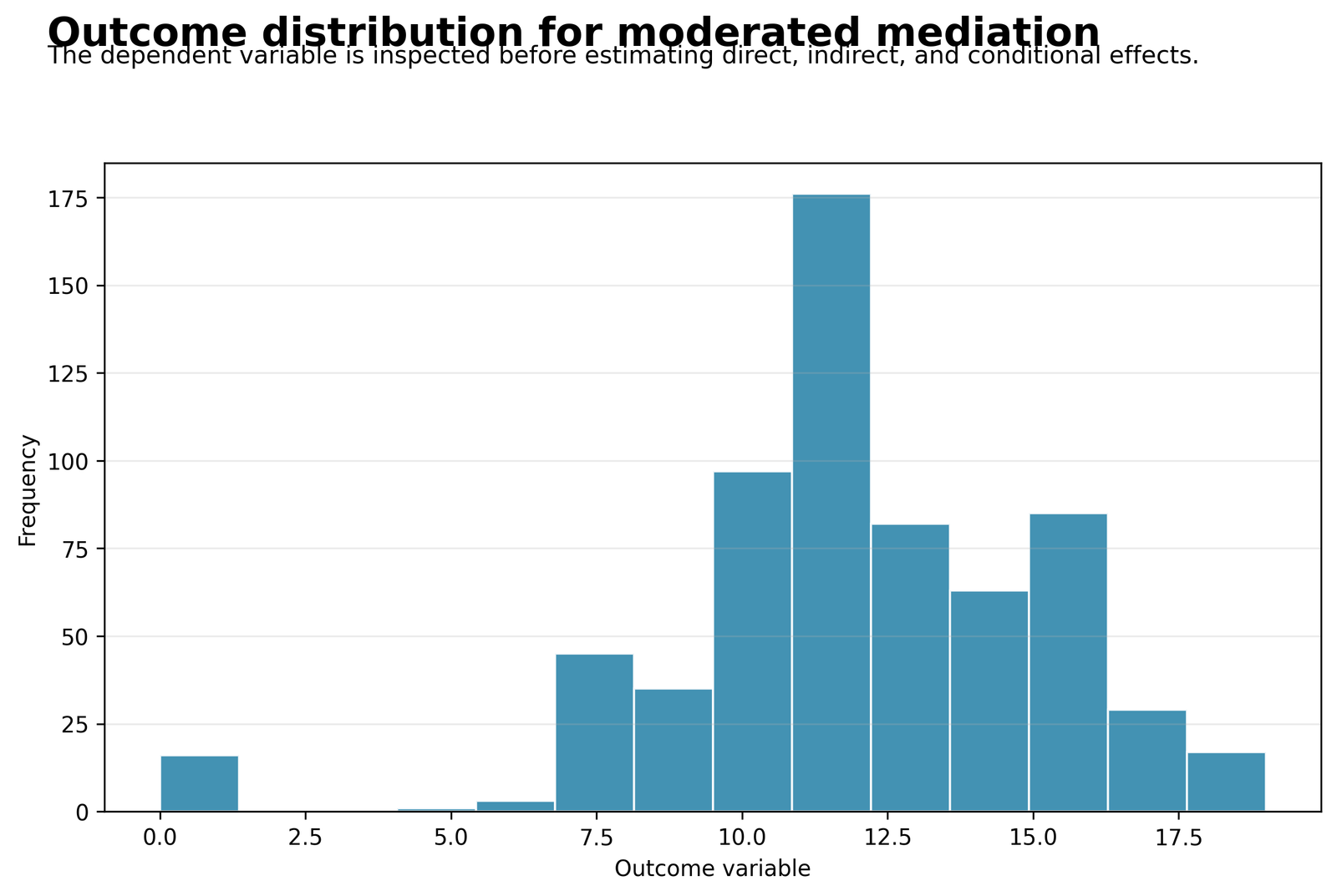
The histogram displays the frequency distribution of final grade G3 before the path models are fitted. This Moderated Mediation interpretation applies to the stated variables, coding and covariate adjustment.
Across 649 students, G3 has mean 11.9060, SD 3.2307, and range 0–19. The largest concentration lies approximately between 10 and 16. This Moderated Mediation interpretation applies to the stated variables, coding and covariate adjustment.
Most students finish with moderate or high final grades, but a small separate group receives zero. The central mass is fairly compact, while the zero-grade cases create an unusually long lower tail that the linear outcome model must handle. This Moderated Mediation interpretation applies to the stated variables, coding and covariate adjustment.
Interpret model fit for the majority grade range and separately inspect the zero-grade cases, because they can create large negative residuals and influence the estimated paths. This Moderated Mediation interpretation applies to the stated variables, coding and covariate adjustment.
Chart 2: Mediator Path from G1 to G2
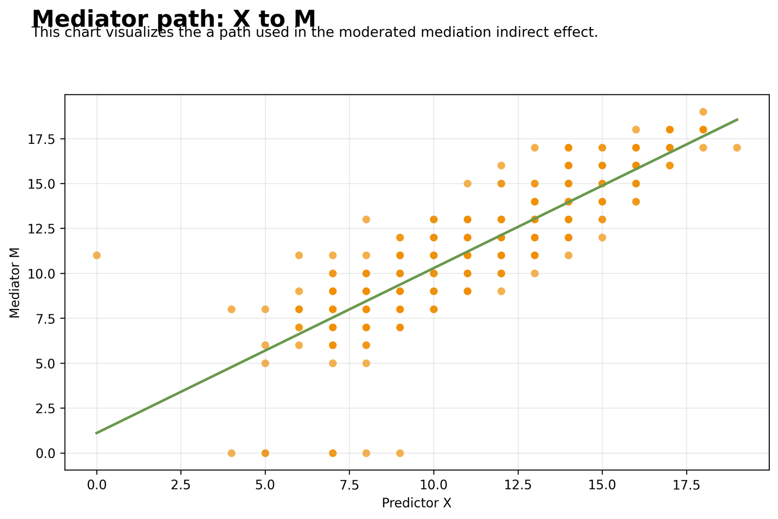
The scatterplot shows G1 on the horizontal axis and mediator G2 on the vertical axis, with the fitted mediator-model line. This Moderated Mediation interpretation applies to the stated variables, coding and covariate adjustment.
The adjusted a path is 0.8860, SE 0.0231, p < .001, 95% CI [0.8407, 0.9313]. The mediator model explains 75.73% of G2 variance. This Moderated Mediation interpretation applies to the stated variables, coding and covariate adjustment.
Students who perform one point better in the first period usually perform almost one point better in the second period, even after failures, absences, age and parental education are controlled. This strong continuity in grades creates a large mediation pathway. This Moderated Mediation interpretation applies to the stated variables, coding and covariate adjustment.
The indirect effect is driven first by this very strong G1-to-G2 link. Check whether G1 and G2 measure sufficiently distinct time points and report their strong overlap when interpreting mediation. This Moderated Mediation interpretation applies to the stated variables, coding and covariate adjustment.
Chart 3: Outcome-Model Path Coefficients
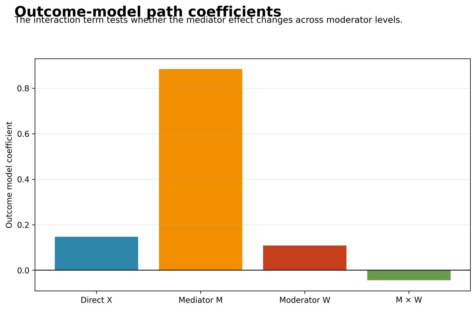
The bars compare the direct G1 effect, the G2 mediator effect, the studytime main effect and the G2-by-studytime interaction. This Moderated Mediation interpretation applies to the stated variables, coding and covariate adjustment.
Direct G1 = 0.1473, G2 = 0.8840, studytime = 0.1084, and G2 × studytime = −0.0441.
Second-period grade is by far the strongest immediate predictor of final grade. G1 still contributes directly, but most of its relationship with G3 operates through G2. The negative interaction means the G2-to-G3 slope becomes slightly weaker as studytime increases. This Moderated Mediation interpretation applies to the stated variables, coding and covariate adjustment.
Describe G2 as the dominant pathway, the direct G1 path as smaller but still present, and the moderation as statistically detectable but modest in size. This Moderated Mediation interpretation applies to the stated variables, coding and covariate adjustment.
Chart 4: Moderation of the G2-to-G3 Path
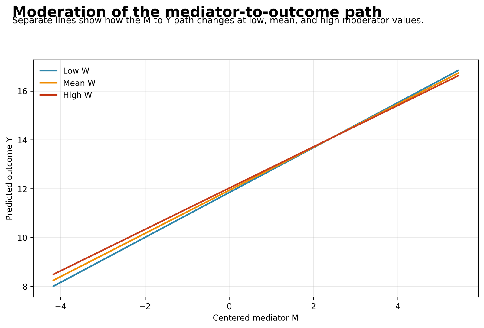
Three fitted lines show the relationship between centered G2 and predicted G3 at low, mean and high studytime. This Moderated Mediation interpretation applies to the stated variables, coding and covariate adjustment.
The conditional G2 slopes are 0.9205 at low studytime, 0.8840 at mean studytime and 0.8474 at high studytime. This Moderated Mediation interpretation applies to the stated variables, coding and covariate adjustment.
Higher G2 predicts higher G3 at every studytime level. The lines are close together, so studytime does not reverse the relationship; it slightly compresses it. At lower G2 values, higher studytime partly offsets weaker grades, whereas at higher G2 values the low-studytime line becomes marginally steeper. This Moderated Mediation interpretation applies to the stated variables, coding and covariate adjustment.
Report a small weakening of the mediator-to-outcome path as studytime rises, not a disappearance of mediation. Avoid presenting the interaction as a large educational difference.
Chart 5: Conditional Indirect Effects
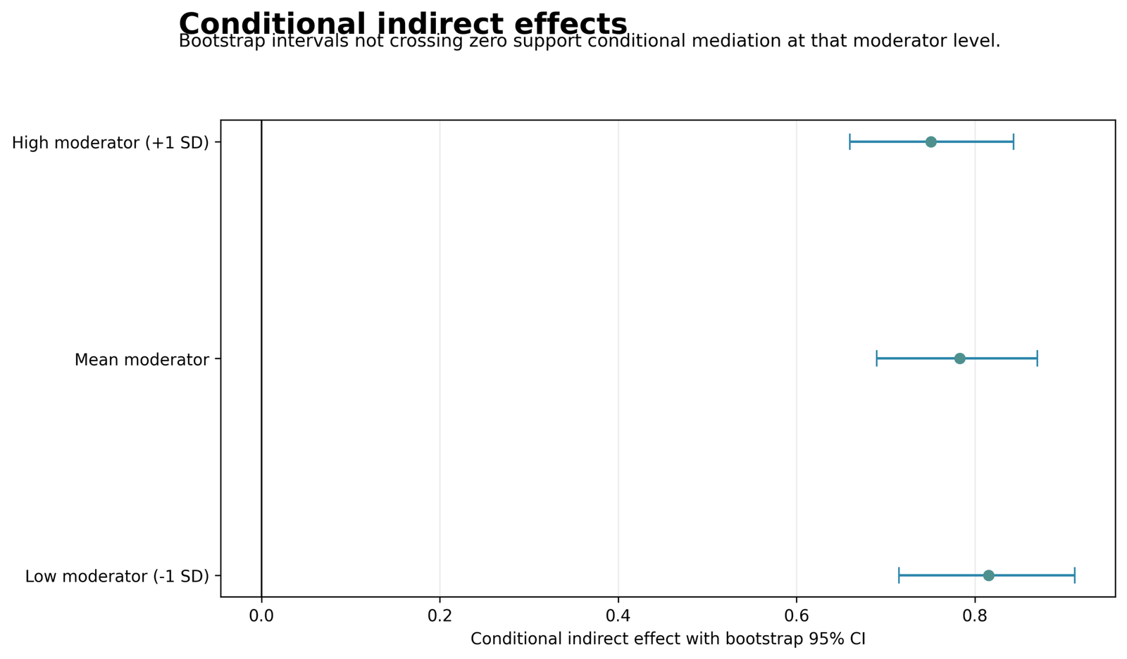
The forest plot shows the estimated G1 → G2 → G3 indirect effect at three studytime levels with bootstrap 95% confidence intervals.
Indirect effects are 0.8156 at low studytime, 0.7832 at the mean and 0.7508 at high studytime. All intervals remain above zero.
G1 affects G3 through G2 for students at every studytime level. The mediated pathway is strongest at lower studytime and weakest at higher studytime, but the decline is gradual and the indirect effect remains substantial throughout.
State that mediation is present across the observed moderator range and that studytime changes its magnitude rather than determining whether mediation exists.
Chart 6: Bootstrap Distribution of the Moderated-Mediation Index
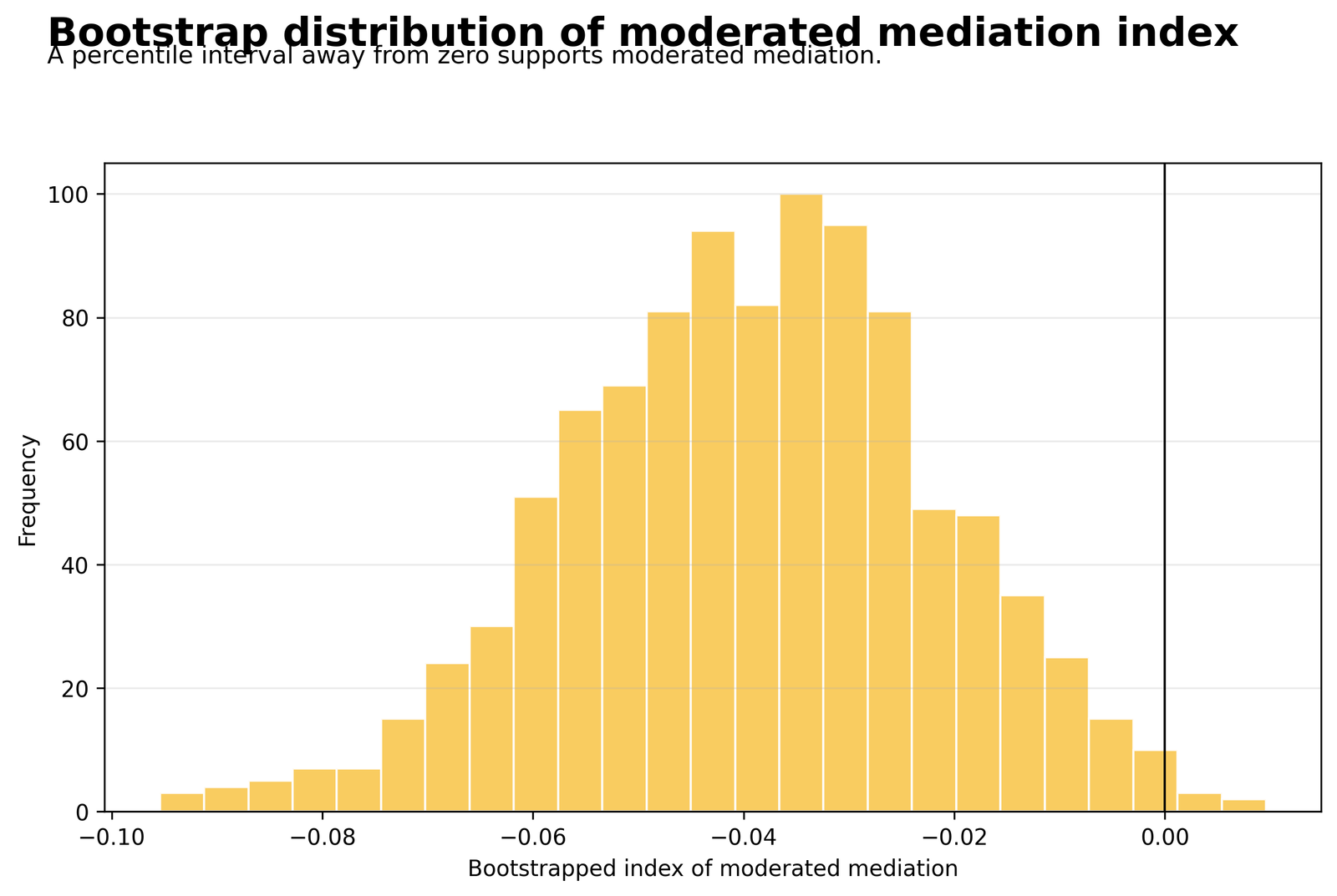
The histogram shows 1,000 bootstrap estimates of the index of moderated mediation, with zero marked as the null value.
The index is −0.0390. The Python percentile 95% CI is [−0.0750, −0.0065]; the R interval is approximately [−0.0740, −0.0049].
Across repeated resamples, the estimated change in the indirect effect is usually negative. The distribution does not merely fluctuate around zero; it consistently indicates that the G1-to-G3 indirect pathway becomes smaller as studytime increases.
Use the bootstrap interval, not only the interaction p-value, as the primary evidence for moderated mediation. The effect is supported statistically but is small in magnitude.
Chart 7: Observed Versus Predicted G3
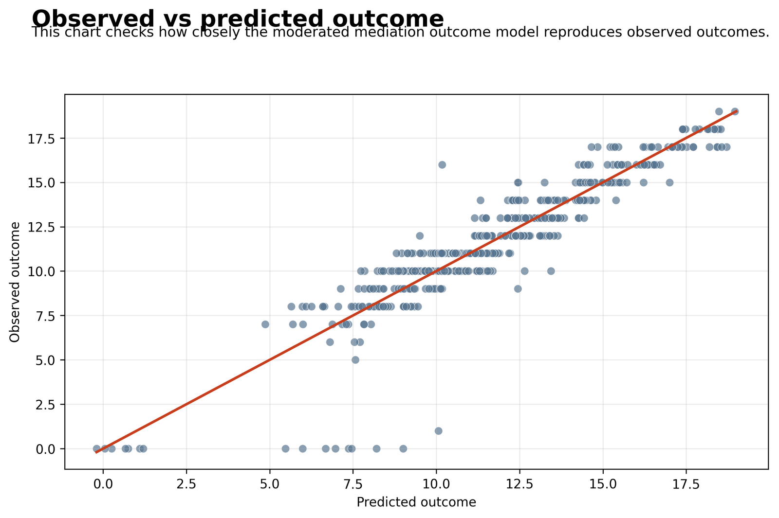
The scatterplot compares observed G3 with values predicted by the full outcome model.
The outcome model has R² = 0.8518, adjusted R² 0.8497 and RMSE 1.2428. Most predictions lie within the 5–19 grade range.
The model reproduces the central and upper grade pattern very closely, which reflects the strong G1 and G2 information. Its largest failures occur for students with observed G3 = 0, because their predictor profiles often resemble students with mid-range predicted grades.
The model is accurate for most students but not for the special zero-grade subgroup. Investigate whether zero grades represent dropout, missing assessment or a distinct process requiring separate modelling.
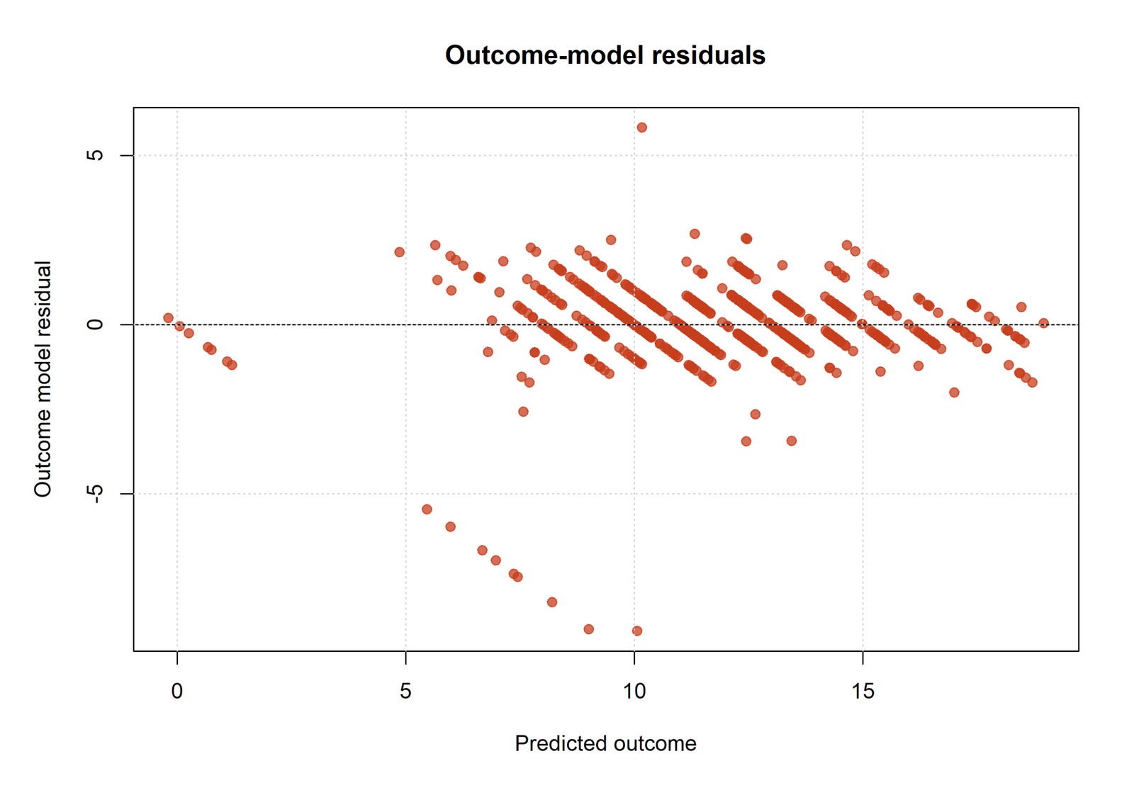
Chart 8: Outcome-Model Residuals
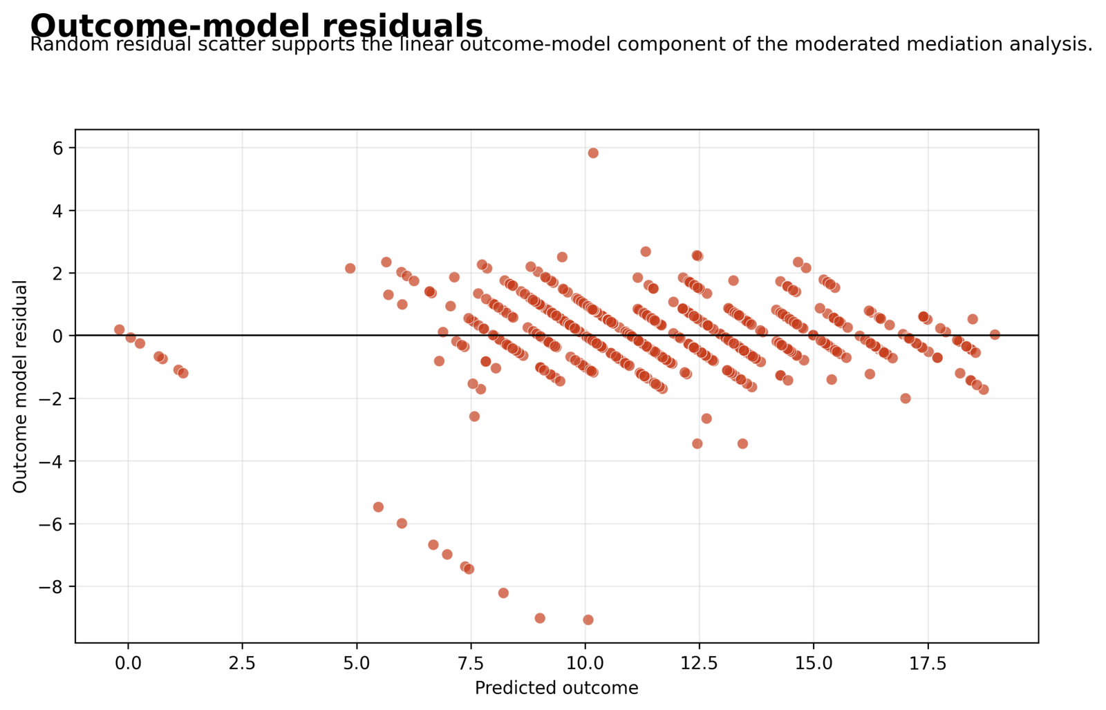
Residuals are plotted against predicted G3 to examine linear-model error patterns.
SPSS residuals range from approximately −8.954 to 5.740, with SD about 1.240. Several residuals below −6 occur around predicted grades 6–10.
Most prediction errors cluster near zero, but the zero-grade students create severe overprediction and a long negative tail. The diagonal bands arise because observed grades are discrete integers, not because the model necessarily has a curved mean relationship.
Inspect influential zero-grade cases, use robust sensitivity analyses and report that residual normality is imperfect even though overall prediction is strong.
R Charts: Two Charts Followed by Two Matching Explanation Boxes
Each R pair is followed by explanation boxes that describe the substantive process represented by the chart rather than simply repeating its values.
R Chart 1: Outcome Distribution for G3
Most students finish with moderate or high final grades, but a small separate group receives zero. The central mass is fairly compact, while the zero-grade cases create an unusually long lower tail that the linear outcome model must handle.
R Chart 2: Mediator Path from G1 to G2
Students who perform one point better in the first period usually perform almost one point better in the second period, even after failures, absences, age and parental education are controlled. This strong continuity in grades creates a large mediation pathway.
R Chart 3: Outcome-Model Path Coefficients
Second-period grade is by far the strongest immediate predictor of final grade. G1 still contributes directly, but most of its relationship with G3 operates through G2. The negative interaction means the G2-to-G3 slope becomes slightly weaker as studytime increases.
R Chart 4: Moderation of the G2-to-G3 Path
Higher G2 predicts higher G3 at every studytime level. The lines are close together, so studytime does not reverse the relationship; it slightly compresses it. At lower G2 values, higher studytime partly offsets weaker grades, whereas at higher G2 values the low-studytime line becomes marginally steeper.
R Chart 5: Conditional Indirect Effects
G1 affects G3 through G2 for students at every studytime level. The mediated pathway is strongest at lower studytime and weakest at higher studytime, but the decline is gradual and the indirect effect remains substantial throughout.
R Chart 6: Bootstrap Distribution of the Moderated-Mediation Index
Across repeated resamples, the estimated change in the indirect effect is usually negative. The distribution does not merely fluctuate around zero; it consistently indicates that the G1-to-G3 indirect pathway becomes smaller as studytime increases.
R Chart 7: Observed Versus Predicted G3
The model reproduces the central and upper grade pattern very closely, which reflects the strong G1 and G2 information. Its largest failures occur for students with observed G3 = 0, because their predictor profiles often resemble students with mid-range predicted grades.
R Chart 8: Outcome-Model Residuals
Most prediction errors cluster near zero, but the zero-grade students create severe overprediction and a long negative tail. The diagonal bands arise because observed grades are discrete integers, not because the model necessarily has a curved mean relationship.
Complete Moderated Mediation Path Results
Mediator model: G2 from G1 and covariates
| Term | B | SE | p | 95% CI | Interpretation |
|---|---|---|---|---|---|
| G1 centered | 0.8860 | 0.0231 | <.001 | 0.8407–0.9313 | Strong positive a path |
| failures | −0.3868 | 0.1081 | .0004 | −0.5991 to −0.1745 | More failures predict lower G2 |
| absences | −0.0020 | 0.0125 | .8760 | −0.0265–0.0226 | Not significant |
| age | 0.1664 | 0.0496 | .0008 | 0.0689–0.2638 | Positive adjusted association |
| Medu | 0.0674 | 0.0664 | .3105 | −0.0630–0.1979 | Not significant |
| Fedu | 0.0583 | 0.0681 | .3916 | −0.0753–0.1920 | Not significant |
Outcome model: G3 from G1, G2, studytime and interaction
| Term | B | SE | p | 95% CI | Interpretation |
|---|---|---|---|---|---|
| G1 centered | 0.1473 | 0.0366 | .0001 | 0.0753–0.2192 | Positive direct effect |
| G2 centered | 0.8840 | 0.0343 | <.001 | 0.8167–0.9513 | Strong mediator-to-outcome path |
| studytime centered | 0.1084 | 0.0622 | .0819 | −0.0137–0.2305 | Main effect not significant |
| G2 × studytime | −0.0441 | 0.0211 | .0370 | −0.0855 to −0.0027 | G2 slope weakens as studytime rises |
| failures | −0.2230 | 0.0952 | .0194 | −0.4099 to −0.0361 | Negative adjusted association |
| absences | 0.0215 | 0.0109 | .0486 | 0.0001–0.0430 | Small positive coefficient |
Use the P-Value and Confidence Interval guides when explaining uncertainty.
Conditional Indirect Effects and Practical Prediction
What remains stable
- G1 strongly predicts G2.
- G2 strongly predicts G3.
- The indirect effect remains positive across studytime.
What changes
- The G2-to-G3 slope declines slightly.
- The indirect effect falls from 0.8156 to 0.7508.
- The change is statistically supported but modest.
For two students who differ by one G1 point but have comparable covariates, the expected G3 difference transmitted through G2 is about 0.816 at low studytime and 0.751 at high studytime. This is a model-based conditional association, not a guaranteed individual change.
Diagnostics and Model Choice
Path-model diagnostics
- Review linearity in both equations
- Check G1–G2 collinearity
- Inspect residual and influence diagnostics
- Verify bootstrap stability
Observed limitations
- Zero-grade cases create large negative residuals
- Condition index reaches 52.52 in the expanded SPSS model
- The interaction effect is small
- Cross-sectional causality remains limited
Use Variance Inflation Factor, Tolerance Statistic, Cook’s Distance, Studentized Residuals and Influence Diagnostics to assess model stability. This Moderated Mediation interpretation should be evaluated with the complete model specification and reported uncertainty.
Residual plots should be interpreted with the discrete 0–19 grade scale. The visible diagonal bands are expected when integer outcomes are regressed on continuous fitted values, but the extreme zero-grade residuals require separate investigation.
SPSS, Python, R and Excel Workflows
Python
Fits the mediator and outcome OLS equations, calculates conditional indirect effects and bootstraps the index.
- 1,000 completed bootstrap samples
- Eight diagnostic charts
- Path and model-fit tables
R
Reproduces the same centered equations and percentile-bootstrap conditional effects.
- Index CI approximately −0.0740 to −0.0049
- Outcome R²=0.8518
- Independent chart validation
SPSS
Uses centered variables, product terms and multiple regression equations with saved predictions and residuals.
- Expanded covariate diagnostics
- Outcome R²≈.853
- Observed versus predicted and residual plots
Excel
Can calculate centered variables, path-based conditional effects and a bootstrap-results summary after coefficients are estimated.
- Center X, M and W
- Calculate M × W
- Evaluate a × (b + qW)
Code: Expand Only the Software You Need
Python Moderated Mediation code
import numpy as np
import pandas as pd
import statsmodels.api as sm

df = pd.read_csv("dataset.csv")
for v in ["G1", "G2", "studytime"]:
    df[v + "_c"] = df[v] - df[v].mean()

df["M_x_W"] = df["G2_c"] * df["studytime_c"]

covars = ["failures", "absences", "age", "Medu", "Fedu"]
X_m = sm.add_constant(df[["G1_c"] + covars])
model_m = sm.OLS(df["G2"], X_m).fit()

X_y = sm.add_constant(
    df[["G1_c", "G2_c", "studytime_c", "M_x_W"] + covars]
)
model_y = sm.OLS(df["G3"], X_y).fit()

a = model_m.params["G1_c"]
b = model_y.params["G2_c"]
q = model_y.params["M_x_W"]
index = a * q

for w in [-df["studytime"].std(), 0, df["studytime"].std()]:
    print(w, a * (b + q * w))
R Moderated Mediation code
df <- read.csv("dataset.csv")
df$G1_c <- df$G1 - mean(df$G1)
df$G2_c <- df$G2 - mean(df$G2)
df$studytime_c <- df$studytime - mean(df$studytime)
df$M_x_W <- df$G2_c * df$studytime_c

m_model <- lm(
  G2 ~ G1_c + failures + absences + age + Medu + Fedu,
  data = df
)

y_model <- lm(
  G3 ~ G1_c + G2_c + studytime_c + M_x_W +
    failures + absences + age + Medu + Fedu,
  data = df
)

a <- coef(m_model)["G1_c"]
b <- coef(y_model)["G2_c"]
q <- coef(y_model)["M_x_W"]
index <- a * q
SPSS Moderated Mediation syntax
DESCRIPTIVES VARIABLES=G1 G2 studytime /SAVE.
COMPUTE G1_c = G1 - 11.3990755.
COMPUTE G2_c = G2 - 11.5701079.
COMPUTE studytime_c = studytime - 1.9306626.
COMPUTE M_x_W = G2_c * studytime_c.
EXECUTE.

REGRESSION
 /DEPENDENT G2
 /METHOD=ENTER G1_c failures absences age Medu Fedu
 /STATISTICS COEFF OUTS CI(95).

REGRESSION
 /DEPENDENT G3
 /METHOD=ENTER G1_c G2_c studytime_c M_x_W
               failures absences age Medu Fedu
 /STATISTICS COEFF OUTS CI(95) COLLIN
 /SAVE PRED RESID.
Excel Moderated Mediation formulas
Centered G1       = G1 - AVERAGE(G1_range)
Centered G2       = G2 - AVERAGE(G2_range)
Centered W        = studytime - AVERAGE(studytime_range)
Interaction       = Centered_G2 * Centered_W
Conditional b     = b_G2 + b_interaction * Centered_W
Indirect effect   = a_path * Conditional_b
Index             = a_path * b_interaction
Advanced Interpretation and Extensions
First-stage versus second-stage moderated mediation
In this model, studytime moderates the second-stage M-to-Y path rather than the G1-to-G2 path. A first-stage model would instead include an X-by-W term in the mediator equation. Compare structures before estimation and justify the moderated path theoretically. See main effects versus interaction effects. This Moderated Mediation interpretation should be evaluated with the complete model specification and reported uncertainty.
Index of moderated mediation
The index equals the a path multiplied by the interaction coefficient. Its bootstrap interval directly tests whether the indirect effect changes with the moderator. The estimated index is −0.0390, indicating a small decline per one-unit increase in centered studytime. Interpret the interval using the confidence interval guide.
Conditional indirect effects
Conditional indirect effects are not separate mediation models. They are evaluations of the same fitted equations at selected moderator values. Low, mean and high studytime produce 0.8156, 0.7832 and 0.7508.
Mean centering
Centering changes the zero point of G1, G2 and studytime, making lower-order coefficients meaningful at the sample mean. Centering does not remove multicollinearity caused by substantive overlap.
Product-term interpretation
The interaction coefficient is the change in the G2 slope for a one-unit increase in centered studytime. Because the coefficient is negative, the mediator-to-outcome slope becomes slightly flatter.
Direct, indirect and total effects
The total effect of G1 on G3 is 0.9339. The direct effect after G2 enters is 0.1473. The difference is represented by the conditional indirect pathway, whose size varies by studytime.
Partial versus complete mediation
The direct effect remains significant, so the model shows partial mediation rather than complete mediation. Complete mediation should never be declared solely because one p-value crosses .05.
Bootstrap percentile intervals
Percentile bootstrap intervals use empirical quantiles of resampled effects. They are especially useful because indirect-effect distributions are often asymmetric and poorly approximated by a normal distribution.
Bias-corrected bootstrap intervals
Bias-corrected intervals adjust for median bias and skewness. They may differ from simple percentile intervals, especially with small samples or highly asymmetric effects.
Number of bootstrap samples
One thousand bootstrap samples provide a usable estimate, but 5,000 or more are commonly preferred for publication when computationally feasible because tail quantiles become more stable.
Johnson-Neyman analysis
A Johnson-Neyman analysis can identify moderator regions where the M-to-Y slope or indirect effect is statistically distinguishable from zero. This extends the three-point evaluation used in simple effects analysis.
Categorical moderators
A categorical moderator requires dummy or effect coding. Conditional indirect effects are then compared across meaningful groups rather than at ±1 SD.
Multiple moderators
Multiple moderators create additional interaction terms and more complex conditional effects. Theory should determine which path each moderator changes.
Multiple mediators
Multiple mediators can be modelled in parallel when each transmits a distinct mechanism. Shared variance among mediators must be interpreted carefully.
Serial mediation
Serial mediation represents a chain such as G1 → study behaviour → G2 → G3. Temporal and causal ordering must be justified before such a model is interpreted.
Parallel mediation
Parallel mediation estimates several indirect pathways simultaneously without imposing an order among mediators.
Moderated direct effects
A moderator can also alter the direct X-to-Y effect. That requires an X-by-W term in the outcome equation in addition to any moderated mediator path.
Covariate selection
Covariates should be chosen because they address a defined confounding or precision question, not because they happen to be available. Unnecessary controls can change the estimand and reduce interpretability.
Temporal ordering
Mediation implies a process over time, yet cross-sectional data do not establish temporal precedence. The grade sequence G1, G2 and G3 provides some ordering, but causal claims still require stronger assumptions.
Measurement error
Measurement error in G1, G2 or studytime can attenuate paths and distort interaction estimates. Latent-variable moderated mediation can address measurement models directly.
Multicollinearity
G1 and G2 are strongly related, so review variance inflation factor and tolerance statistics. A high condition index in SPSS may partly reflect the intercept and centered grade structure.
Heteroskedasticity
Use the Breusch-Pagan test and residual plots to evaluate unequal variance. Bootstrap inference protects the indirect effect more than it protects every coefficient estimate.
Influential observations
Large negative residuals from zero-grade cases may influence the outcome equation. Review Cook’s distance and influence diagnostics before deleting any case.
Power for conditional indirect effects
Power depends on the product of the a path and the moderated b-path change. Small interaction effects often require large samples. Plan simulations and consult statistical power rather than relying on a simple events-per-variable rule.
Causal interpretation
Moderated mediation estimates conditional associations unless treatment assignment, temporal order, no-unmeasured-confounding assumptions and correct model specification support causal interpretation.
Cross-validation and replication
Replication should evaluate the index, conditional indirect effects and calibration of the outcome equation in another cohort. Resampling within one dataset cannot establish transportability.
APA-Style Reporting
The conditional indirect effects were 0.816 at low studytime, 0.783 at mean studytime and 0.751 at high studytime; all bootstrap intervals excluded zero. The direct G1 effect remained significant, B = 0.147, SE = 0.037, p < .001. The outcome model explained 85.18% of G3 variance. This Moderated Mediation interpretation should be evaluated with the complete model specification and reported uncertainty.
Report exact p-values, confidence intervals, the moderator values and the bootstrap method. Avoid saying that studytime causes the indirect effect to weaken unless the causal assumptions are defensible.
Publication Checklist and Common Mistakes
Include in the final report
- X, M, W and Y definitions
- Centered-variable method
- Mediator and outcome equations
- a, b, c′ and interaction paths
- Conditional indirect effects
- Bootstrap index and CI
- Model fit and residual diagnostics
Avoid these errors
- Calling one interaction a complete conditional process
- Reporting only low, mean and high effects without the index
- Interpreting the moderator main effect as moderation
- Claiming causation from cross-sectional regressions
- Ignoring influential zero-grade cases
- Equating significance with a large effect
Review the Null and Alternative Hypothesis, Type I and Type II Error and Statistical Power guides when planning replication.
Downloads
Frequently Asked Questions
What is Moderated Mediation?
What is the index of moderated mediation?
Which path is moderated here?
What are X, M, W and Y?
Is the indirect effect significant at all studytime levels?
Does higher studytime eliminate mediation?
Why is the interaction negative?
Is the moderator main effect significant?
What does the direct effect mean?
Why use bootstrap confidence intervals?
How many bootstrap samples were used?
Can Moderated Mediation prove causation?
What is the difference from moderated regression?
Why center the variables?
How should the zero-grade cases be handled?
How is Moderated Mediation reported?
Final Moderated Mediation Conclusion
The analysis supports a strong G1 → G2 → G3 indirect pathway and a small negative moderation of the G2-to-G3 segment by studytime. The indirect effect remains positive and statistically supported at low, mean and high studytime.
The practical message is not that studytime removes the value of prior achievement. Instead, the transmission of G1 through G2 is slightly less steep at higher studytime. The index is statistically reliable, but the conditional effects remain close in magnitude.

