
Lasso Selection + Ridge Shrinkage + Cross-Validated Prediction
Elastic Net Regression: Formula, Interpretation, Python, R, SPSS and Excel Guide
Elastic Net Regression combines L1 and L2 regularization to predict a continuous outcome while shrinking weak coefficients and selecting useful predictors. This worked guide predicts final grade G3 for 649 students, names every variable, reports exact Python and R results, explains all supplied charts with their real values, and provides SPSS, Python, R and Excel workflows.
Quick Answer: Elastic Net Regression Result
The Python model predicted the continuous outcome G3 using eight numeric variables—G1, G2, studytime, failures, absences, age, Medu, and Fedu—plus five categorical variables—school, sex, address, famsize, and Pstatus. One-hot encoding produced 13 predictor columns. The analysis used 486 training rows, 163 test rows, and 5-fold cross-validation.
Cross-validation selected l1_ratio = 1.0000 and alpha/lambda = 0.084017. Five coefficients remained non-zero: G2 = 2.5841, G1 = 0.2783, failures = −0.0546, school_MS = −0.0487, and sex_M = −0.0212. Test performance was RMSE = 1.2675, MAE = 0.7774, and R² = 0.8491.
Main interpretation: both Python and R show strong out-of-sample prediction of G3. Python produced the sparser solution, retaining only five terms, with G2 carrying by far the largest standardized coefficient.
Important qualification: Python and R used different encoded predictor counts, folds, splits, and alpha values. Their performance numbers should be presented as separate validated workflows, not merged into one model.
Table of Contents
- What Is Elastic Net Regression?
- Elastic Net vs Lasso vs Ridge Regression
- Elastic Net Formula and Objective Function
- When to Use Elastic Net Regression
- Assumptions and Practical Checks
- Variables Used and Data Dictionary
- Python Model Settings and Results
- Python Chart-by-Chart Interpretation
- R Model Settings and Results
- R Chart-by-Chart Validation
- SPSS Elastic Net Workflow
- Excel Worked Example
- SPSS, Python, R and Excel Workflows
- Code Blocks
- How Alpha and Lambda Are Selected
- How to Interpret Elastic Net Coefficients
- How to Compare Elastic Net with Ordinary Regression
- Detailed Diagnostic Review
- Research Questions Elastic Net Can Answer
- APA-Style Reporting
- Common Mistakes
- Downloads
- Related Salar Cafe Guides
- FAQs
What Is Elastic Net Regression?
Elastic Net Regression is a regularized regression method for continuous outcomes. It adds two penalties to the ordinary least-squares loss: an L1 penalty that can force coefficients to zero and an L2 penalty that continuously shrinks coefficients. The combination is useful when a dataset contains many predictors, correlated predictors, dummy variables, or a risk of overfitting.
In this example, the model predicts G3, the final student grade. The penalties determine which academic and demographic variables retain predictive value after accounting for the others. The selected Python solution is effectively lasso because l1_ratio equals 1, while the selected R solution is a true Elastic Net blend because alpha equals 0.9.
Simple definition: Elastic Net keeps useful predictors, shrinks unstable coefficients, and can set weak predictors to zero while selecting the penalty by cross-validation.
Elastic Net vs Lasso vs Ridge Regression
| Method | Penalty | Can Set Coefficients to Zero? | Best Use |
|---|---|---|---|
| Ordinary linear regression | None | No | Low-dimensional data with limited multicollinearity and low overfitting risk. |
| Lasso regression | L1 | Yes | Sparse variable selection when only a subset of predictors is needed. |
| Ridge regression | L2 | Usually no | Stabilizing correlated predictors while retaining them. |
| Elastic Net Regression | L1 + L2 | Yes | Variable selection plus stability when predictors are correlated. |
The mixing value controls the balance. In Python’s convention, l1_ratio = 1 is pure lasso and 0 is ridge. In R glmnet, alpha = 1 is lasso and 0 is ridge. Values between 0 and 1 create a true Elastic Net combination.
Elastic Net Regression Formula and Objective Function
The first term is prediction error. The L1 component, Σ|βⱼ|, promotes sparsity and variable selection. The L2 component, Σβⱼ², shrinks correlated coefficients smoothly. λ controls overall penalty strength, while α or l1_ratio controls the lasso–ridge mixture.
| Parameter | Meaning | Result in This Post |
|---|---|---|
| λ / alpha penalty | Overall shrinkage strength. | Python 0.084017; R 0.07909967. |
| α / l1_ratio | Balance between L1 and L2 penalties. | Python 1.0; R 0.9. |
| Non-zero coefficient | Predictor retained by the selected penalized model. | Python 5 of 13; R 16 of 41. |
| Zero coefficient | Predictor removed under the selected penalty. | Eight Python terms were shrunk to zero. |
When to Use Elastic Net Regression
Elastic Net is appropriate when the dependent variable is continuous and the predictor set is moderately or highly dimensional, contains correlated measures, includes many dummy variables, or requires automated shrinkage and selection. In this dataset, G1 and G2 are strongly related academic predictors, while the categorical fields generate multiple encoded columns. Elastic Net can stabilize this structure while identifying the strongest predictive subset.
Use Binary Logistic Regression instead when the outcome has two categories. Use Elastic Net linear regression when the outcome remains numeric, as G3 does here.
Assumptions and Practical Checks
| Check | Meaning | How It Applies Here |
|---|---|---|
| Continuous outcome | The target should be numeric for Elastic Net linear regression. | G3 is a continuous grade score. |
| Independent observations | Rows should not be repeated measurements treated as independent. | Each row represents one student. |
| Standardization | Predictors must be comparable before penalization. | Numeric and encoded predictors were scaled before Python fitting. |
| Encoding | Categorical variables require dummy or one-hot columns. | school, sex, address, famsize and Pstatus were encoded. |
| Cross-validation | Penalty settings should be selected out of sample. | Python used 5 folds; R used 10 folds. |
| Residual structure | Residuals should not show strong curves or funnels. | Most residuals are near zero, with several large negative exceptions. |
| Multicollinearity | Elastic Net handles correlation better than unpenalized regression, but interpretation still requires care. | Review multicollinearity, VIF, and tolerance. |
Classical coefficient p-values are not the main basis for selecting penalized predictors. Cross-validated prediction error and stability are more important than testing every coefficient against zero.
Variables Used and Data Dictionary
| Variable | Role | Meaning and Coding | Python Status |
|---|---|---|---|
| G3 | Continuous outcome | Final grade predicted by Elastic Net; observed mean about 11.91. | Outcome |
| G1 | Numeric predictor | First-period grade. | Retained, coefficient +0.2783. |
| G2 | Numeric predictor | Second-period grade. | Retained, coefficient +2.5841. |
| studytime | Numeric/ordinal predictor | Weekly study-time group. | Shrunk to zero. |
| failures | Numeric predictor | Number of previous class failures. | Retained, coefficient −0.0546. |
| absences | Numeric predictor | Number of school absences. | Shrunk to zero. |
| age | Numeric predictor | Student age in years. | Shrunk to zero. |
| Medu | Numeric/ordinal predictor | Mother’s education level. | Shrunk to zero. |
| Fedu | Numeric/ordinal predictor | Father’s education level. | Shrunk to zero. |
| school_MS | Dummy predictor | 1 for MS school; GP is reference. | Retained, coefficient −0.0487. |
| sex_M | Dummy predictor | 1 for male; female is reference. | Retained, coefficient −0.0212. |
| address_U | Dummy predictor | 1 for urban; rural is reference. | Shrunk to zero. |
| famsize_LE3 | Dummy predictor | 1 for family size of three or fewer; GT3 is reference. | Shrunk to zero. |
| Pstatus_T | Dummy predictor | 1 when parents live together; apart is reference. | Shrunk to zero. |
Coefficient scale: the reported Python slopes are standardized coefficients because the predictors were scaled before model fitting. The intercept, 11.7798, is the expected G3 prediction when the standardized predictors equal zero and reference categories apply.
Python Elastic Net Model Settings and Results
| Python Setting or Result | Value | Interpretation |
|---|---|---|
| Rows used | 649 | No rows were lost after cleaning. |
| Train / test rows | 486 / 163 | 75% training and 25% testing. |
| Encoded predictors | 13 | Eight numeric plus five dummy-coded categorical effects. |
| Cross-validation folds | 5 | Penalty selected using five internal folds. |
| Selected l1_ratio | 1.0000 | The chosen grid point is pure lasso. |
| Selected penalty | 0.084017 | Cross-validated alpha/lambda strength. |
| Non-zero coefficients | 5 of 13 | A sparse selected model. |
| Train RMSE / MAE / R² | 1.2518 / 0.7775 / 0.8476 | Strong in-sample prediction. |
| Test RMSE / MAE / R² | 1.2675 / 0.7774 / 0.8491 | Strong and stable out-of-sample performance. |
| Baseline test RMSE / MAE / R² | 1.2509 / 0.7593 / 0.8530 | Unpenalized regression is slightly more accurate but less sparse. |
Python Standardized Coefficient Table
| Term | Standardized Coefficient | Direction | Selection |
|---|---|---|---|
| Intercept | 11.7798 | Intercept | Model intercept |
| G2 | +2.5841 | Positive | Retained |
| G1 | +0.2783 | Positive | Retained |
| failures | −0.0546 | Negative | Retained |
| school_MS | −0.0487 | Negative | Retained |
| sex_M | −0.0212 | Negative | Retained |
| absences, studytime, Medu, age, Fedu, address_U, famsize_LE3, Pstatus_T | 0.0000 | Zero | Shrunk to zero |
Python Chart-by-Chart Interpretation with Real Data Values
The Python report generated seven charts. The explanations below use the actual outcome, sample sizes, selected hyperparameters, coefficient values, error measures, and visible diagnostic ranges rather than generic descriptions.
Python Chart 1: Outcome Distribution for G3
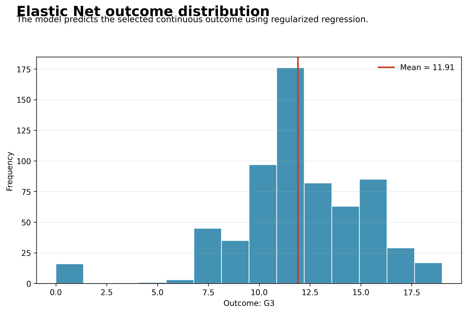
The dependent variable is G3, the final student grade measured from 0 to 19 in the analyzed data. All 649 rows were retained after cleaning. The histogram’s vertical reference line marks the observed mean of 11.91; the underlying worked data give a more precise mean of approximately 11.906 and a standard deviation of about 3.231. Most G3 values are concentrated between roughly 9 and 16, with the tallest bar around grades 11–12.
The chart also shows a small low-score group at or close to 0 and fewer observations near the upper end of 18–19. Because Elastic Net predicts a continuous outcome, this distribution matters: the model is learning the full numeric G3 scale rather than a pass/fail category. The wide but concentrated range supports regression, while the small cluster of very low grades helps explain several larger residuals in the diagnostic chart.
Python Chart 2: Observed vs Predicted Test Values
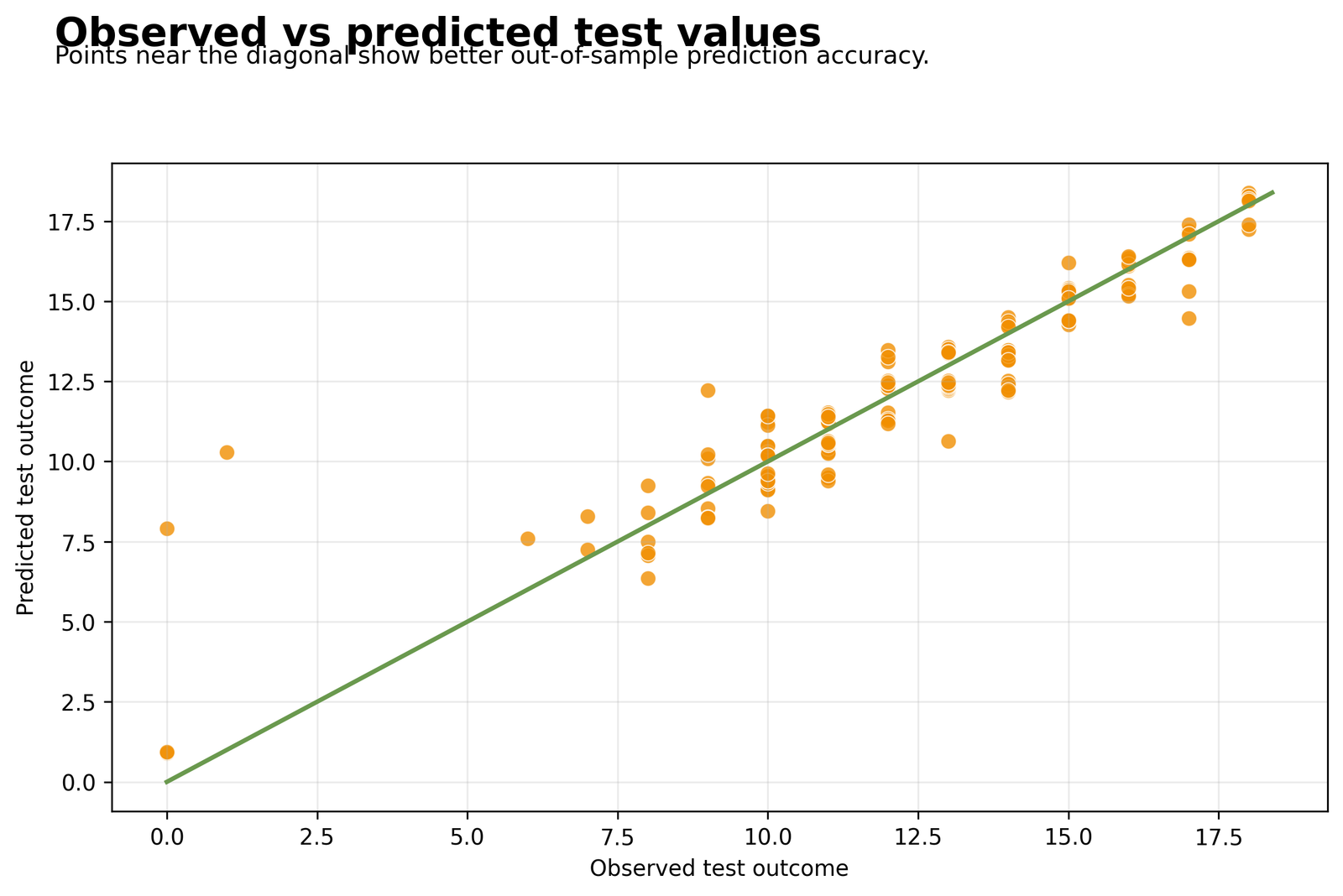
This scatterplot compares the 163 observed G3 test values with their Elastic Net predictions. Points near the diagonal represent accurate out-of-sample predictions. The Python test model achieved RMSE = 1.2675, MAE = 0.7774, and R² = 0.8491. Thus, predictions were typically less than one grade point away in absolute terms, while the model explained about 84.91% of test-set variation in G3.
The strongest agreement appears from observed grades of approximately 8 to 19. The most visible departures occur at the lower end: an observed G3 of 0 is predicted near 8, another observed 0 is predicted near 1, and an observed value around 1 is predicted above 10. These unusual cases increase RMSE more strongly than MAE because squared error gives large misses extra weight. The chart therefore supports strong overall prediction but also indicates that rare very low outcomes are difficult for the selected linear regularized structure.
Python Chart 3: Residuals vs Predicted Test Values
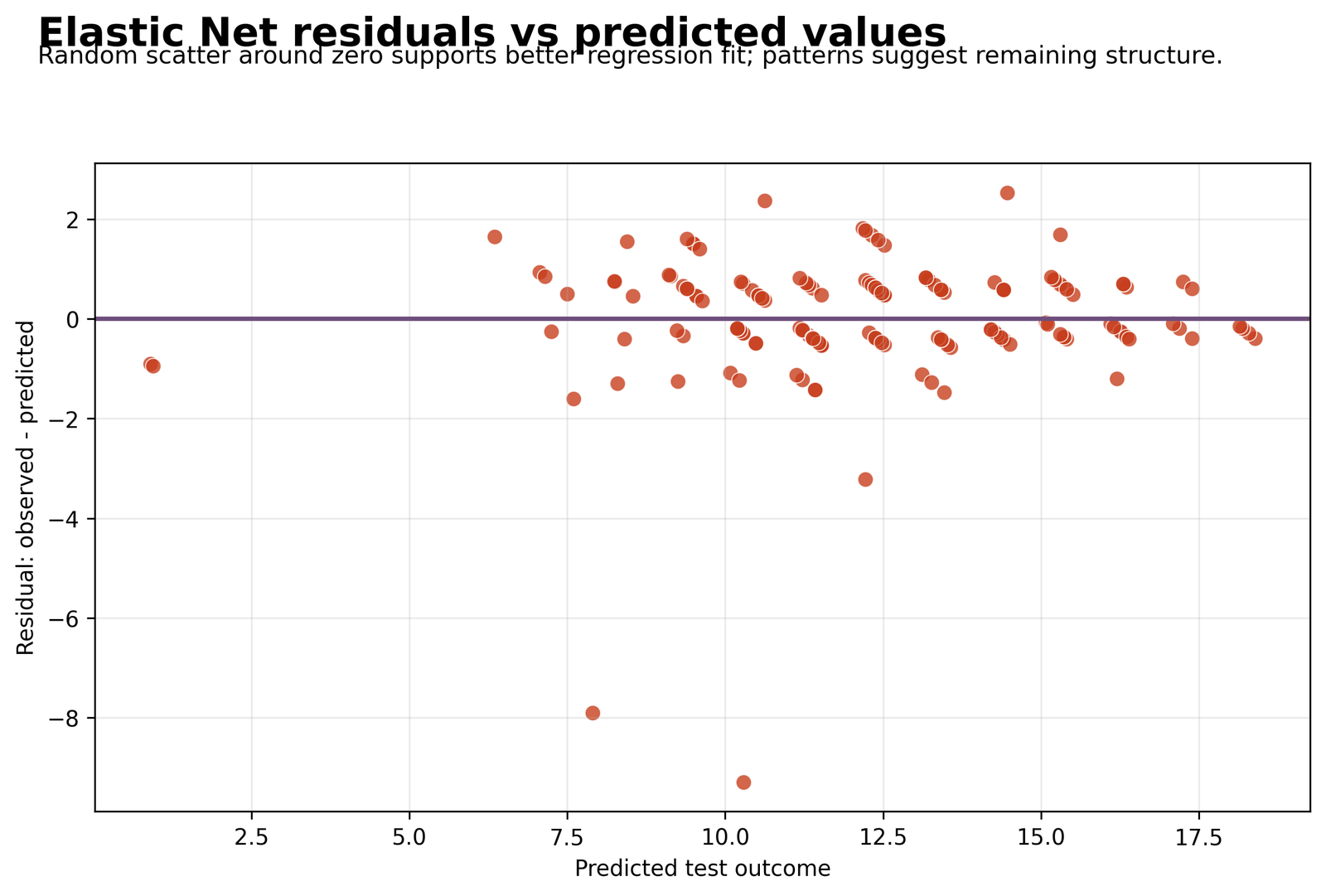
Residuals are calculated as observed G3 minus predicted G3. Most of the 163 test residuals lie between approximately −2 and +2 and are distributed on both sides of the zero line. This agrees with the relatively low test MAE of 0.7774 and suggests that the model does not systematically overpredict or underpredict the majority of students.
However, the plot contains two large negative residuals near −7.9 and −9.3, plus another around −3.2. A negative residual means predicted G3 exceeded observed G3, so these cases are students whose actual final grades were much lower than their prior information suggested. Positive residuals reach roughly +2.5. The mostly horizontal cloud supports reasonable fit, but the extreme negative cases should be checked with studentized residuals, Cook’s distance, and influence diagnostics.
Python Chart 4: Retained Coefficient Sizes After Shrinkage
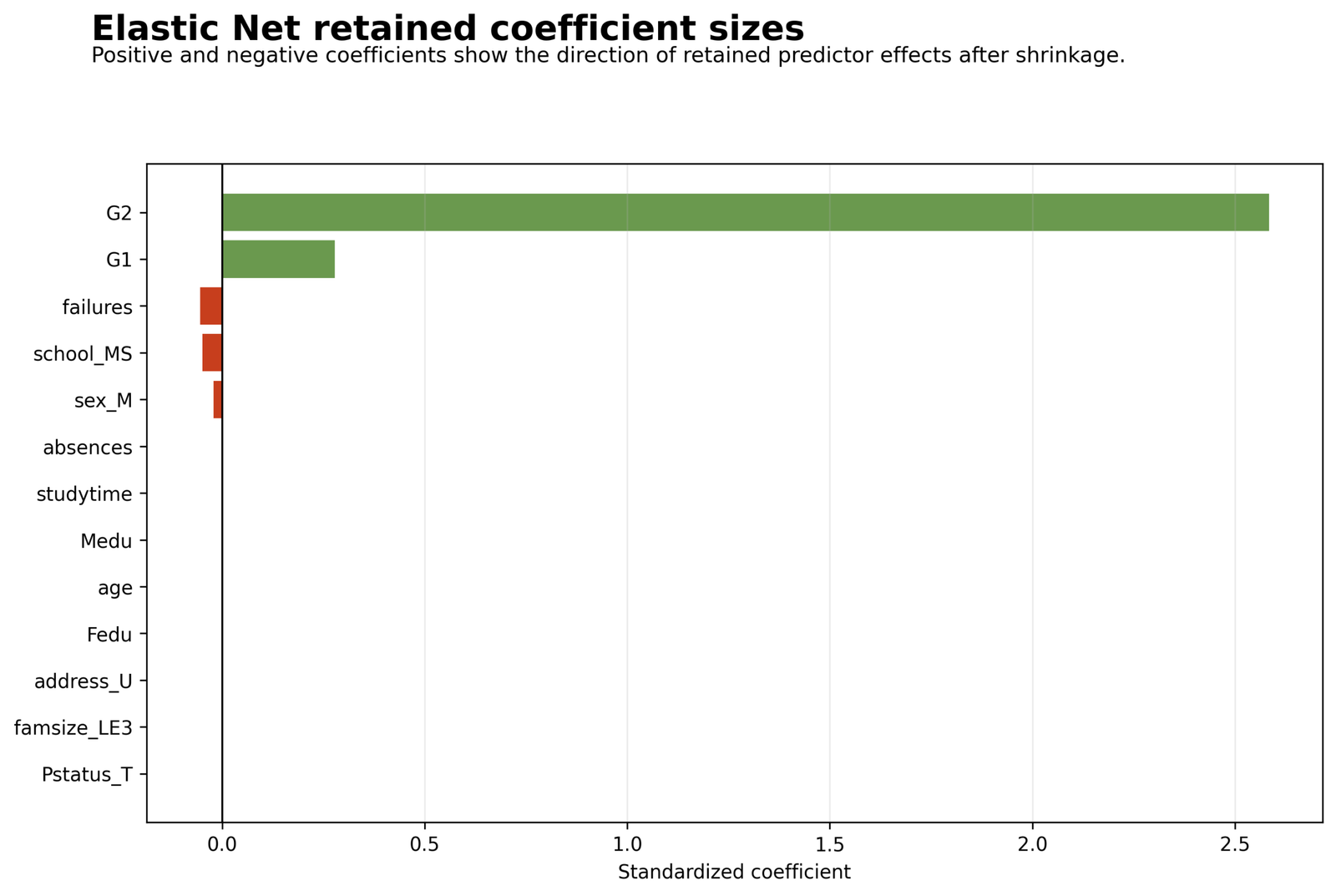
The Python model began with 13 encoded predictors and retained only 5 non-zero coefficients after regularization. Because continuous variables were standardized before fitting, coefficient magnitudes can be compared as relative predictive contributions. G2, the second-period grade, dominates with a standardized coefficient of +2.5841. G1, the first-period grade, is also retained at +0.2783.
The remaining retained effects are much smaller and negative: failures = −0.0546, school_MS = −0.0487, and sex_M = −0.0212. The penalty reduced absences, studytime, Medu, age, Fedu, address_U, famsize_LE3, and Pstatus_T to zero. The chart does not prove that zeroed variables have no relationship with G3; it shows that they added insufficient incremental predictive value after the model accounted for stronger correlated predictors, especially G2 and G1.
Python Chart 5: Cross-Validation Curve for the Selected Mixing Ratio
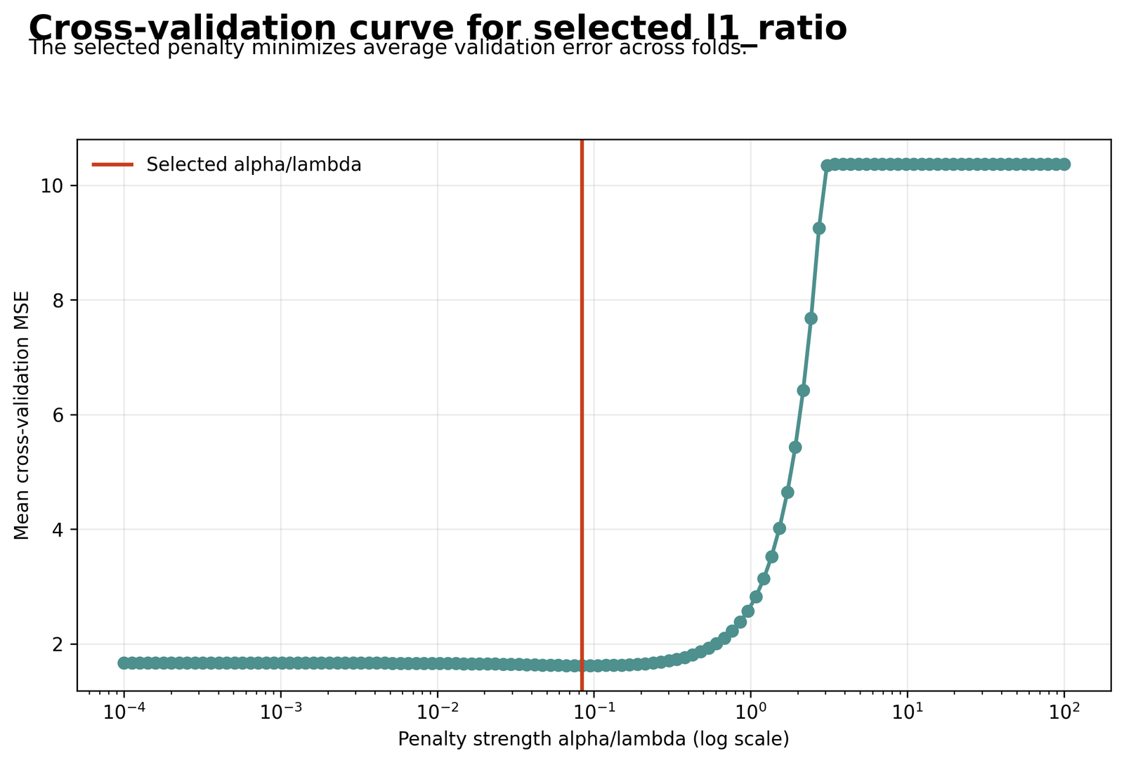
The cross-validation curve shows mean validation MSE across candidate penalty strengths on a logarithmic scale. Python used 5-fold cross-validation and selected alpha/lambda = 0.084017. The chosen mixing value was l1_ratio = 1.0000, so the selected point is the lasso end of the Elastic Net grid. The vertical line lies near the bottom of the error valley, where mean cross-validation MSE is approximately 1.6.
At very small penalties, validation error remains close to the minimum but more coefficients remain active. As the penalty rises above roughly 0.2–0.5, validation MSE increases, and beyond about 1 it rises sharply toward 4, 6, 8, and eventually above 10. This demonstrates the bias–variance trade-off: excessive shrinkage removes useful grade information, while the selected penalty achieves low validation error with only five retained predictors.
Python Chart 6: Train and Test Prediction Error
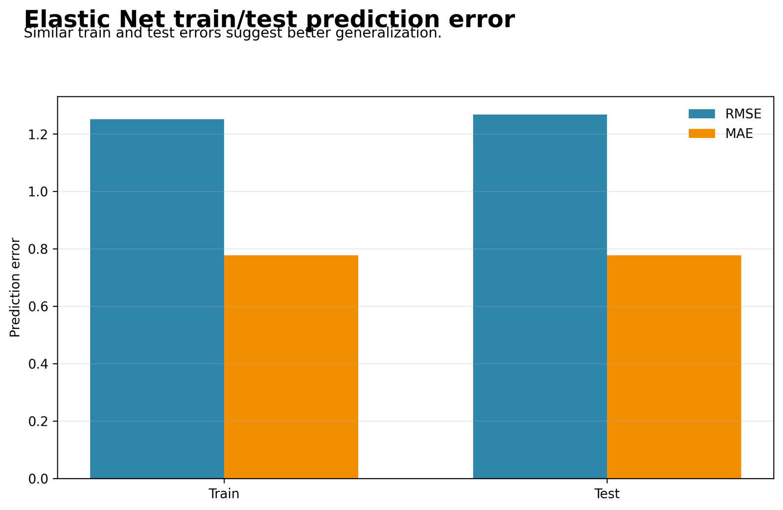
The train/test error chart shows very similar performance across the two data partitions. For the 486 training rows, Elastic Net produced RMSE = 1.2518 and MAE = 0.7775. For the 163 test rows, RMSE was 1.2675 and MAE was 0.7774. The train-to-test RMSE increase is only 0.0157, while MAE differs by just 0.0001.
This near equality provides strong evidence of stable generalization rather than severe overfitting. Training R² was 0.8476 and test R² was slightly higher at 0.8491. The ordinary linear-regression baseline was marginally better on test RMSE (1.2509) and R² (0.8530), but Elastic Net achieved a much sparser model by retaining only five of thirteen encoded predictors. The practical benefit is therefore parsimony and variable selection rather than a large raw-accuracy gain over unpenalized regression.
Python Chart 7: Elastic Net Regularization Path
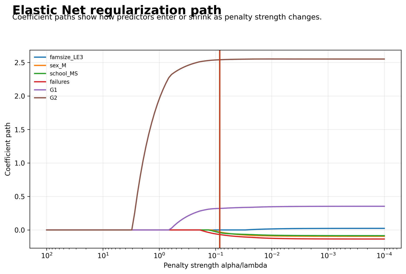
The regularization path traces standardized coefficients as penalty strength changes. At very large penalties near 100, all coefficients are zero. As the penalty weakens, G2 enters first and grows toward approximately +2.58; G1 then increases toward approximately +0.28. The selected penalty is marked at 0.084017.
At the selected line, five paths remain non-zero: G2, G1, failures, school_MS, and sex_M. G2’s path is far larger than every other predictor, demonstrating that second-period grade carries most of the model’s predictive information for final grade G3. The paths for failures and school_MS move slightly below zero, while sex_M remains only weakly negative. The chart also shows why regularization is useful in correlated academic data: related predictors can enter, shrink, or disappear as the penalty changes.
R Elastic Net Model Settings and Results
The R workflow is a separate validation model. It uses the same outcome G3 and 649 rows but creates 41 model.matrix columns, uses a 487/162 train/test split, applies 10-fold cross-validation, and selects a predominantly lasso Elastic Net mixture.
| R Setting or Result | Value | Interpretation |
|---|---|---|
| Rows used | 649 | Complete analyzed sample. |
| Predictor columns after model.matrix | 41 | Broader encoded feature space than Python. |
| Train / test rows | 487 / 162 | Separate R split. |
| Cross-validation folds | 10 | More folds than Python. |
| Best lambda | 0.07909967 | Selected penalty strength. |
| Best alpha mixing | 0.9 | 90% lasso and 10% ridge contribution. |
| Non-zero selected coefficients | 16 | Less sparse than the Python solution. |
| Test MAE | 0.78911 | Average absolute error below one grade point. |
| Test RMSE | 1.10875 | Low out-of-sample squared-error scale. |
| Test R² | 0.881831 | 88.18% of test variation explained. |
| Adjusted R² using non-zero features | 0.868792 | Strong adjusted predictive performance. |
R Chart-by-Chart Validation
All seven supplied R chart placements are included below. Where the R PDF provides exact numerical values, those values are integrated into the narrative. The Python and R results remain separated because their feature matrices and tuning procedures differ.
R Chart 1: Outcome Distribution for G3
The R analysis uses the same continuous outcome, G3, and all 649 available rows. Its report expands the design matrix to 41 predictor columns, so the R model includes a broader one-hot-encoded predictor space than the 13-column Python specification. The observed G3 distribution remains the same, including the mean near 11.91 and the concentration of scores around 9–16.
Because the outcome itself does not change across software, this chart should be interpreted identically: R predicts final grade on its original numeric scale. The difference between the Python and R models comes from predictor encoding, train/test split, cross-validation folds, and selected penalty—not from a different dependent variable.
R Chart 2: Observed vs Predicted Test Values
R trained on 487 rows and evaluated 162 test rows. The R report gives MAE = 0.78911, RMSE = 1.10875, and R² = 0.881831. These results indicate that the R predictions were, on average, about 0.79 grade points from the observed G3 values and explained 88.18% of test-set variance.
The R test results are stronger than the Python test results of RMSE 1.2675 and R² 0.8491, but they are not a strict head-to-head comparison because R used 41 encoded columns, 10-fold cross-validation, 162 test rows, and a different random split. The appropriate conclusion is that both workflows show strong out-of-sample prediction, not that one language is inherently superior.
R Chart 3: Residuals vs Predicted Test Values
The R residual interpretation should be tied to its reported test errors: RMSE = 1.10875 and MAE = 0.78911. The modest MAE indicates that most residuals are small, while the larger RMSE shows that a limited number of larger misses still affect squared error. Residuals should ideally form a random horizontal band around zero without a funnel or curve.
Any extreme negative residuals represent students whose observed G3 was far below the R prediction, while positive residuals represent underprediction. These cases should be reviewed rather than automatically removed, especially because rare low final grades can be legitimate. The same internal diagnostic guides for outlier detection and influence analysis apply to the R model.
R Chart 4: Retained Coefficient Sizes After Shrinkage
The R report states that 16 coefficients remained non-zero out of 41 model-matrix columns. This is a less sparse solution than Python’s 5 of 13 because R selected alpha = 0.9, retaining a small ridge component, and used a broader encoded predictor matrix. The R chart should therefore be read as a variable-selection summary for its own specification rather than as a duplicate of the Python five-variable solution.
R’s selected model still demonstrates the core Elastic Net principle: influential predictors retain non-zero coefficients, weak redundant predictors are heavily shrunk, and some are set to zero. The coefficient table generated in the R output folder should be used to identify the exact 16 retained terms; the supplied R PDF reports the count but does not list their individual estimates.
R Chart 5: Cross-Validation Curve for the Selected Mixing Ratio
R used 10-fold cross-validation and selected lambda = 0.07909967 with an alpha mixing value of 0.9. Alpha 0.9 means the penalty is predominantly lasso-like but still includes a 10% ridge component. That small ridge component can stabilize groups of correlated predictors and helps explain why R retained 16 terms rather than Python’s five.
The selected lambda is close in scale to Python’s 0.084017, so both workflows locate the useful penalty region near 0.08. The exact values should not be expected to match because the cross-validation folds, train/test split, encoded feature count, and alpha grid differ.
R Chart 6: Train and Test Prediction Error
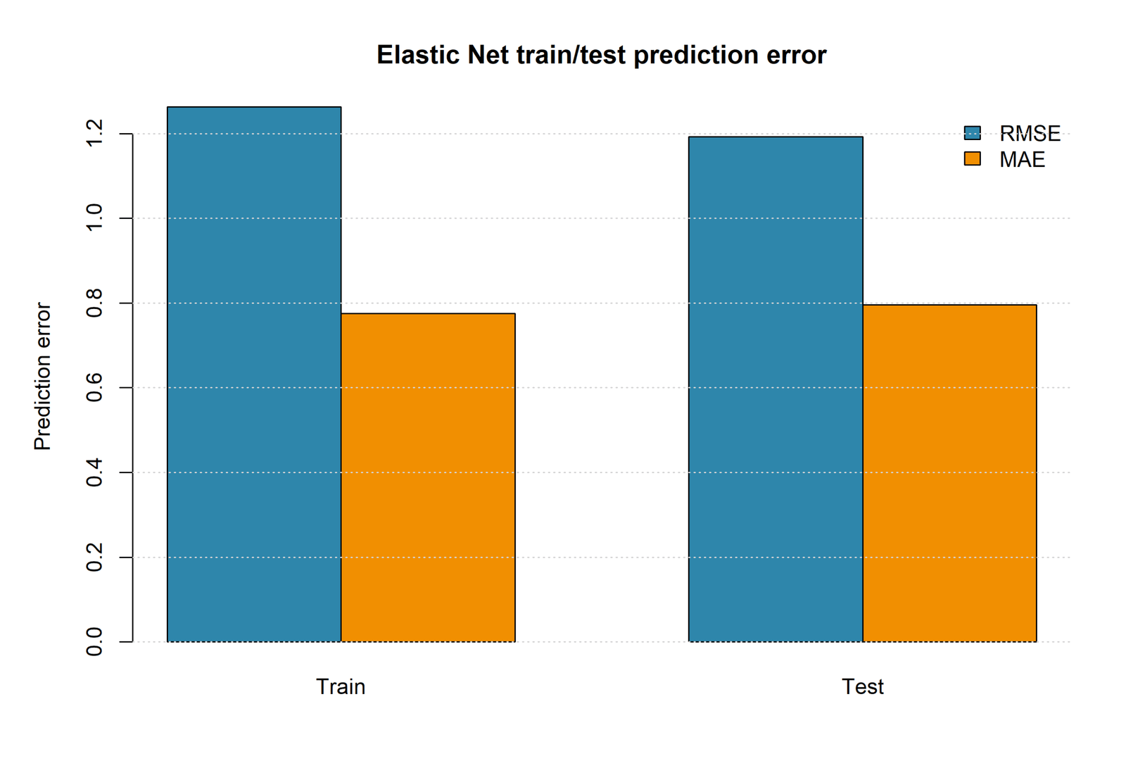
The R model’s reported test errors are MAE = 0.78911 and RMSE = 1.10875. Its test R² is 0.881831, and adjusted R² calculated using the non-zero features is 0.868792. These values indicate strong predictive performance after accounting for the 16 retained coefficients.
The supplied R report does not provide a numerical training-error row, so the public interpretation should not invent one. The valid evidence is that the 162-row test set achieved low error and high explained variance. Train/test balance can be discussed from the generated chart, but only the reported R test statistics should be quoted as exact.
R Chart 7: Elastic Net Regularization Path
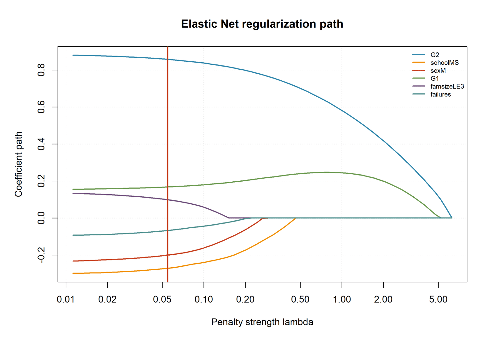
The R regularization path is governed by the selected alpha = 0.9 and lambda = 0.07909967. At strong penalties, coefficient paths approach zero; as lambda decreases, more terms enter the model. At the selected lambda, 16 of 41 encoded coefficients remain active.
This path is especially useful when predictors are correlated, because Elastic Net can retain related variables together more readily than pure lasso. The result should be interpreted as a predictive selection process, not as a classical significance test: a non-zero coefficient is selected by cross-validation, whereas a zero coefficient is excluded under the chosen penalty.
SPSS Elastic Net Regression Workflow and Interpretation
Standard SPSS linear-regression menus do not estimate an Elastic Net penalty directly. A practical SPSS workflow uses SPSS Python integration to import the prepared data, one-hot encode categorical variables, standardize predictors, fit cross-validated Elastic Net, write predictions and coefficients back to SPSS, and save SAV, SPV and PDF output.
Asset check: the supplied SPSS PDF URL belongs to Cox Regression, not Elastic Net Regression, so it has deliberately not been embedded or interpreted in this article. Mixing that Cox output into an Elastic Net post would be statistically incorrect.
| SPSS Output Item | What to Report | How to Interpret It |
|---|---|---|
| Outcome and predictor list | G3 plus all numeric and categorical predictors. | Confirms the analysis variables and coding. |
| Standardization | Means and standard deviations or standardized design matrix. | Required so the penalty treats predictor scales fairly. |
| Selected alpha and l1_ratio | Cross-validated tuning values. | Describe penalty strength and lasso–ridge balance. |
| Retained coefficients | Terms with non-zero standardized slopes. | Selected predictors under the chosen penalty. |
| Train/test metrics | RMSE, MAE and R². | Measures predictive error and generalization. |
| Residual diagnostics | Residual plots and unusual cases. | Identifies remaining structure and large misses. |
Excel Worked Example Explained
The worked Excel file demonstrates the Elastic Net objective using editable coefficients. Its example uses G1, G2, studytime and failures for 12 illustrative observations. The workbook shows standardized predictors, predicted G3, residuals, squared residuals, L1 penalty, L2 penalty, and the total Elastic Net objective.
Download the Elastic Net Regression worked Excel file
| Excel Input or Result | Worked Value | Meaning |
|---|---|---|
| Lambda penalty | 0.20 | Illustrative penalty strength. |
| Alpha mix / l1_ratio | 0.70 | 70% lasso and 30% ridge mix. |
| Intercept | 11.50 | Baseline prediction in the worked example. |
| Std G1 coefficient | 0.85 | Positive retained example coefficient. |
| Std G2 coefficient | 1.25 | Largest positive worked coefficient. |
| Std studytime coefficient | 0.25 | Small positive example effect. |
| Std failures coefficient | −0.80 | Negative example effect. |
| MSE | 0.432224 | Average squared residual in the illustrative rows. |
| L1 penalty | 0.441000 | λ × α × sum of absolute coefficients. |
| L2 penalty | 0.089625 | λ × (1−α)/2 × sum of squared coefficients. |
| Elastic Net objective | 0.962849 | MSE + L1 penalty + L2 penalty. |
Excel Formula Logic
Predicted G3:
=Intercept
 + Coef_Std_G1*Std_G1
 + Coef_Std_G2*Std_G2
 + Coef_Std_Studytime*Std_Studytime
 + Coef_Std_Failures*Std_Failures

Residual:
=Actual_G3-Predicted_G3

Squared residual:
=Residual^2

MSE:
=AVERAGE(Squared_Residual_Range)

L1 penalty:
=Lambda*Alpha_Mix*SUM(ABS(Coefficient_Range))

L2 penalty:
=Lambda*(1-Alpha_Mix)/2*SUMSQ(Coefficient_Range)

Elastic Net objective:
=MSE+L1_Penalty+L2_Penalty
SPSS, Python, R and Excel Workflows for Elastic Net Regression
| Software | Recommended Workflow | Main Output |
|---|---|---|
| Python | Use ColumnTransformer, OneHotEncoder, StandardScaler and ElasticNetCV. | Selected penalty, standardized coefficients, predictions, residuals, RMSE, MAE, R² and seven charts. |
| R | Use model.matrix and glmnet/cv.glmnet with an alpha grid. | Selected alpha and lambda, non-zero coefficients, test metrics, path and CV charts. |
| SPSS | Use embedded Python to fit the regularized model and write results back to SPSS. | SAV data, Viewer output, PDF, coefficient and prediction tables. |
| Excel | Use standardized columns and formulas to demonstrate prediction and the Elastic Net objective. | Worked calculations and a transparent teaching example. |
Code Blocks for Elastic Net Regression
Python Code
import numpy as np
import pandas as pd
from sklearn.compose import ColumnTransformer
from sklearn.linear_model import ElasticNetCV
from sklearn.metrics import mean_absolute_error, mean_squared_error, r2_score
from sklearn.model_selection import train_test_split
from sklearn.pipeline import Pipeline
from sklearn.preprocessing import OneHotEncoder, StandardScaler

df = pd.read_csv("dataset.csv")

outcome = "G3"
numeric = ["G1", "G2", "studytime", "failures",
           "absences", "age", "Medu", "Fedu"]
categorical = ["school", "sex", "address", "famsize", "Pstatus"]

X = df[numeric + categorical]
y = df[outcome]

X_train, X_test, y_train, y_test = train_test_split(
    X, y, test_size=0.25, random_state=42
)

preprocess = ColumnTransformer([
    ("num", StandardScaler(), numeric),
    ("cat", OneHotEncoder(drop="first", handle_unknown="ignore"), categorical)
])

model = ElasticNetCV(
    l1_ratio=[0.1, 0.3, 0.5, 0.7, 0.9, 1.0],
    alphas=np.logspace(-4, 2, 120),
    cv=5,
    max_iter=100000
)

pipeline = Pipeline([
    ("preprocess", preprocess),
    ("model", model)
])

pipeline.fit(X_train, y_train)
pred = pipeline.predict(X_test)

print("Selected l1_ratio:", pipeline.named_steps["model"].l1_ratio_)
print("Selected alpha:", pipeline.named_steps["model"].alpha_)
print("RMSE:", mean_squared_error(y_test, pred) ** 0.5)
print("MAE:", mean_absolute_error(y_test, pred))
print("R-squared:", r2_score(y_test, pred))
R Code
library(glmnet)

df <- read.csv("dataset.csv")
y <- df$G3
x <- model.matrix(
  G3 ~ .,
  data = df
)[, -1]

set.seed(42)
test_id <- sample(seq_len(nrow(df)), size = round(0.25 * nrow(df)))
x_train <- x[-test_id, ]
x_test  <- x[test_id, ]
y_train <- y[-test_id]
y_test  <- y[test_id]

alpha_grid <- seq(0.1, 1.0, by = 0.1)
cv_models <- lapply(alpha_grid, function(a) {
  cv.glmnet(x_train, y_train, alpha = a, nfolds = 10)
})

best_index <- which.min(sapply(cv_models, function(m) min(m$cvm)))
best_alpha <- alpha_grid[best_index]
best_cv <- cv_models[[best_index]]
best_lambda <- best_cv$lambda.min

pred <- as.numeric(predict(
  best_cv, newx = x_test, s = "lambda.min"
))

rmse <- sqrt(mean((y_test - pred)^2))
mae <- mean(abs(y_test - pred))
r_squared <- 1 - sum((y_test - pred)^2) /
  sum((y_test - mean(y_test))^2)

print(best_alpha)
print(best_lambda)
print(rmse)
print(mae)
print(r_squared)
SPSS Syntax with Embedded Python Pattern
SET PRINTBACK=OFF MPRINT=OFF RESULTS=ON DECIMAL=DOT.
OUTPUT CLOSE ALL.
OUTPUT NEW NAME=ElasticNetOutput.
OUTPUT ACTIVATE ElasticNetOutput.

GET DATA
  /TYPE=TXT
  /FILE='D:\DATA ANALYSIS\H Regression Tests and Models\Elastic Net Regression\dataset.csv'
  /ENCODING='UTF8'
  /DELCASE=LINE
  /DELIMITERS=","
  /ARRANGEMENT=DELIMITED
  /FIRSTCASE=2
  /IMPORTCASE=ALL.

DATASET NAME ElasticNetData.
EXECUTE.

BEGIN PROGRAM Python3.
# Read active SPSS data, create encoded standardized predictors,
# fit sklearn ElasticNetCV, and write coefficients/predictions
# to SPSS datasets or CSV tables.
END PROGRAM.

OUTPUT SAVE
  OUTFILE='D:\DATA ANALYSIS\H Regression Tests and Models\Elastic Net Regression\SPSS_Output\spv\Elastic-Net-Regression.spv'.

OUTPUT EXPORT
  /CONTENTS EXPORT=ALL LAYERS=PRINTSETTING MODELVIEWS=PRINTSETTING
  /PDF DOCUMENTFILE='D:\DATA ANALYSIS\H Regression Tests and Models\Elastic Net Regression\SPSS_Output\pdf\Elastic-Net-Regression-SPSS-Output.pdf'.
How Alpha and Lambda Are Selected in Elastic Net Regression
Elastic Net has two tuning decisions. The first is the overall penalty strength, commonly written as lambda in R and often exposed as alpha by Python’s scikit-learn implementation. The second is the mixing value, called alpha in R and l1_ratio in Python. These names can be confusing because the same word, alpha, refers to different quantities in the two software ecosystems. A careful report should therefore state both the software and the parameter meaning.
In the Python analysis, the cross-validation grid examined mixing values from 0.1 to 1.0 and penalty strengths distributed across a logarithmic sequence. Five-fold cross-validation selected l1_ratio = 1.0000 and a penalty of 0.084017. An l1 ratio of 1 means the selected Python solution is located at the lasso end of the Elastic Net continuum. The method was still estimated through ElasticNetCV, but cross-validation concluded that no ridge component was needed for this particular 13-column design matrix.
In the R analysis, the candidate alpha values ranged across the lasso–ridge continuum and ten-fold cross-validation selected alpha = 0.9 with lambda = 0.07909967. This means the R penalty was composed of approximately 90% L1 and 10% L2. The small ridge contribution helps correlated predictors remain together more readily than under pure lasso, which is one reason the R model retained 16 of 41 encoded terms while Python retained 5 of 13.
Why Cross-Validation Is Necessary
A penalty chosen only because it produces the smallest training error would usually be too weak. A very small penalty allows the model to fit noise and retain unstable predictors. A penalty that is too large creates the opposite problem: useful coefficients are pushed toward zero, predictions become overly similar to the mean, and both bias and test error rise. Cross-validation estimates prediction error on observations not used to fit each temporary model, making the selected penalty more defensible.
The Python cross-validation curve shows a broad low-error region around penalty values close to 0.08. At the selected value of 0.084017, mean validation MSE is near its minimum, approximately 1.6. As the penalty rises above roughly 0.2 to 0.5, validation error begins to increase. Penalties above approximately 1 produce much larger error because G2, G1, and other useful signals are excessively shrunk.
Minimum-Error Rule vs One-Standard-Error Rule
Many Elastic Net workflows offer two common choices. The minimum-error rule selects the lambda with the lowest mean cross-validation error. The one-standard-error rule selects the strongest penalty whose error remains within one standard error of the minimum. The second option usually produces a simpler model with fewer retained variables, but it may sacrifice a small amount of predictive accuracy.
The Python workflow used the minimum-error solution produced by ElasticNetCV. The R workflow reported the selected lambda associated with the best cross-validated performance. If a more compact research model were required, the analyst could also inspect a one-standard-error lambda and compare its retained-variable count, RMSE, MAE, and R² with the current results.
| Tuning Quantity | Python Result | R Result | Interpretation |
|---|---|---|---|
| Overall penalty | 0.084017 | 0.07909967 | Both workflows selected a useful penalty region close to 0.08. |
| L1/L2 mixing value | l1_ratio = 1.0 | alpha = 0.9 | Python selected pure lasso; R retained a small ridge contribution. |
| Cross-validation folds | 5 | 10 | R used more folds, while Python used larger validation subsets per fold. |
| Encoded feature count | 13 | 41 | The broader R model matrix allows more terms to enter the regularized solution. |
| Non-zero coefficients | 5 | 16 | The number retained depends on both the feature matrix and selected penalty. |
How to Interpret Elastic Net Coefficients Correctly
Elastic Net coefficients are interpreted differently from ordinary least-squares coefficients when the predictors have been standardized. In the Python workflow, numeric and dummy-coded predictors were passed through a standardized preprocessing pipeline before the model was fitted. Consequently, the reported coefficient for a numeric predictor represents the expected change in predicted G3 associated with a one-standard-deviation increase in that predictor, while holding the remaining standardized columns constant.
The largest coefficient is G2 = +2.5841. This does not mean that one raw grade point in G2 increases G3 by 2.5841 points. Instead, it means that a one-standard-deviation increase in standardized G2 is associated with an increase of about 2.584 predicted G3 points, conditional on the other encoded predictors. Because G2 is measured on the same 0–20 academic scale as G3 but was standardized during estimation, the standardized interpretation must be preserved.
The coefficient for G1 = +0.2783 is much smaller. G1 therefore retains some incremental predictive information after G2 is included, but G2 accounts for most of the academic signal. This is reasonable because G2 is measured closer in time to the final G3 outcome. The two grade variables are also correlated, so regularization distributes and shrinks their effects rather than estimating them as unrelated pieces of information.
The retained negative coefficient for failures = −0.0546 indicates a small reduction in predicted G3 as prior failures increase, after standardization and adjustment. The coefficients for school_MS = −0.0487 and sex_M = −0.0212 are also negative but very small. Their retention means cross-validation found some predictive contribution under the selected penalty; it does not automatically establish a causal, practically important, or statistically significant difference.
How to Interpret Zero Coefficients
Eight Python terms were shrunk exactly to zero: absences, studytime, Medu, age, Fedu, address_U, famsize_LE3, and Pstatus_T. A zero coefficient means that, under the selected cross-validated penalty and in the presence of the retained variables, the predictor did not improve prediction enough to justify a non-zero slope. It does not prove that the predictor has no bivariate association with G3 and does not prove that it is unimportant in every population or alternative model.
For example, absences may correlate with final grade in a simple analysis, yet become zero after G1, G2, and failures enter the penalized model. This can happen because the stronger academic variables already capture much of the predictive information that absences contributes. The correct wording is therefore “absences was shrunk to zero in the selected Elastic Net model,” not “absences has no effect on final grade.”
Standardized vs Original-Scale Coefficients
Standardized coefficients help compare predictor importance, but original-scale coefficients are easier for many readers to understand. To obtain original-scale slopes, analysts can transform the standardized model back using each predictor’s training-set mean and standard deviation. Dummy variables require additional care because standardizing a 0/1 column changes the contrast scale. The published report should clearly identify whether coefficients are standardized, unstandardized, or transformed back to the original units.
The intercept of 11.7798 is also conditional on preprocessing. It represents the expected G3 when standardized numeric and encoded predictors equal zero, with reference-category coding embedded in the transformed design. It should not be interpreted simply as the mean grade of a literal student with every raw predictor equal to zero.
Interpretation rule: a retained coefficient is a cross-validated predictive contribution, not a classical significance test and not proof of causality. Direction, magnitude, stability, subject-matter meaning, and external validation should all be considered together.
How to Compare Elastic Net with Ordinary Linear Regression
The Python workflow fitted an ordinary linear-regression baseline to the same training and test split. On the test set, the unpenalized baseline produced RMSE = 1.2509, MAE = 0.7593, and R² = 0.8530. Elastic Net produced RMSE = 1.2675, MAE = 0.7774, and R² = 0.8491. The ordinary model is therefore slightly better on all three raw test metrics.
The difference is small. Elastic Net RMSE is only 0.0166 grade points higher than the baseline, MAE is 0.0181 higher, and R² is lower by only 0.0039. In return, Elastic Net reduces the 13-column predictor set to only five non-zero terms. This is the central trade-off: the regularized model sacrifices a very small amount of test accuracy to obtain a substantially simpler and potentially more stable predictor set.
Why a Slightly Less Accurate Elastic Net Model Can Still Be Useful
A sparse model is easier to communicate, reproduce, and monitor. It reduces dependence on weak predictors, limits the number of coefficients that must be maintained, and may generalize better when future datasets differ slightly from the original sample. In educational prediction, a model based mainly on G2, G1, failures, school, and sex may be easier to explain than a full model that assigns small slopes to every available variable.
However, simplicity should not be presented as automatic superiority. If the primary objective is minimum prediction error on a closely matched population, the unpenalized model’s small advantage may be relevant. If the objective is variable selection, coefficient stability, or reducing the predictor set, Elastic Net offers a clearer benefit.
Train–Test Stability
Elastic Net’s training RMSE was 1.2518 and test RMSE was 1.2675, a difference of only 0.0157. Training MAE was 0.7775 and test MAE was 0.7774, essentially identical. Training R² was 0.8476 and test R² was 0.8491. These closely matched values indicate that the selected penalty did not create a large overfitting gap.
The slightly higher test R² does not imply that the test set was used to tune the model. Small reversals can occur because random splits differ in outcome variability and case difficulty. The important point is that training and test metrics are highly similar, supporting stable performance across the two partitions.
| Model | Test RMSE | Test MAE | Test R² | Predictor Complexity |
|---|---|---|---|---|
| Ordinary linear regression | 1.2509 | 0.7593 | 0.8530 | All encoded predictors retained. |
| Python Elastic Net | 1.2675 | 0.7774 | 0.8491 | 5 of 13 coefficients retained. |
| R Elastic Net | 1.10875 | 0.78911 | 0.881831 | 16 of 41 coefficients retained on a different split. |
The R row should not be used as a direct software competition because it is based on a different test split and broader feature matrix. It is included to document the separate R validation workflow, not to claim that R intrinsically outperforms Python.
Detailed Diagnostic Review of the Elastic Net Model
Regularization reduces coefficient variance but does not eliminate the need for diagnostics. A penalized model can still produce nonlinear residual patterns, heteroskedastic errors, influential observations, unstable performance across subgroups, or poor predictions at the extremes of the outcome distribution. The supplied charts provide several diagnostic clues that should be discussed together.
Observed vs Predicted Pattern
The Python test scatterplot shows close agreement for most students between observed G3 values and predicted values. The main cloud follows the diagonal from approximately G3 = 8 through G3 = 19. The strongest mismatches occur among rare low outcomes. At least one observed G3 of 0 is predicted around 8, another observed 0 is predicted around 1, and an observed grade near 1 is predicted above 10.
These cases indicate regression toward the center. Because most students have final grades near the middle and upper part of the distribution, the model has stronger information for that region. Very low final grades are uncommon, so a linear regularized model may predict them too high when their G1 and G2 values do not reflect the later collapse in performance.
Residual Distribution and Extreme Errors
Most test residuals lie between approximately −2 and +2, consistent with MAE below one grade point. The two most extreme negative residuals are approximately −7.9 and −9.3. These values mean the model overpredicted the corresponding G3 outcomes by nearly eight and nine grade points. Such errors are practically important even when the average performance is strong.
Analysts should identify the underlying rows and inspect G1, G2, failures, absences, and any unusual contextual variables. A large residual can represent a data-entry mistake, an exceptional event, an omitted variable, or a legitimate but difficult case. It should not be removed merely because it is inconvenient. Useful companion checks include studentized residuals, Cook’s distance, Mahalanobis distance, and influence diagnostics.
Linearity and Missing Nonlinear Structure
Elastic Net linear regression assumes that the selected transformed predictors combine linearly to predict G3. Regularization does not automatically model curves, thresholds, interactions, or changing slopes. If residuals form a curve against predicted values, analysts should consider polynomial terms, restricted splines, interactions, or a Bayesian regression formulation with more flexible prior structure.
One plausible nonlinear feature is the relationship between G2 and G3 near the pass boundary. The linear coefficient for G2 is dominant, but students with identical G2 scores may experience very different final outcomes. Interactions between G2 and failures, studytime, school, or absences could capture some of this heterogeneity. Any expanded model must be tuned and evaluated on held-out data rather than accepted solely because training error decreases.
Heteroskedasticity and Error Spread
The residual plot should also be examined for a funnel shape. A widening spread at higher predictions would indicate non-constant error variance. In the supplied plot, most residuals form a fairly even horizontal band, but the rare low-grade observations create an asymmetric lower tail. Formal checks such as the Breusch–Pagan test or White test may be applied to an unpenalized diagnostic model, while robust or bootstrap uncertainty can be used when classical variance assumptions are doubtful.
Validation Beyond One Random Split
The current Python model uses one 75/25 split with five-fold cross-validation inside the training set. This is a sound introductory design, but repeated cross-validation or nested cross-validation would provide a more stable estimate of performance. Repeating the split across multiple random seeds would show whether the selected five-term solution is stable or whether weak variables enter and leave across samples.
External validation is even more important. The model was trained on one student dataset with a specific grading system and school context. Before operational use, it should be tested on later cohorts or independent schools. A model can perform well internally yet lose accuracy when grade distributions, teaching practices, missing-data patterns, or student characteristics change.
Research Questions Elastic Net Regression Can Answer
Elastic Net is most useful when the research goal combines prediction with reduction of a large or correlated predictor set. It does not replace causal design or classical inference, but it can answer several practical questions clearly.
| Research Question | Elastic Net Output | Result in This Example |
|---|---|---|
| How accurately can final grade G3 be predicted? | Held-out RMSE, MAE, and R². | Python test RMSE 1.2675, MAE 0.7774, R² 0.8491. |
| Which predictors remain useful after accounting for the others? | Non-zero penalized coefficients. | G2, G1, failures, school_MS, and sex_M remained in Python. |
| Which predictor contributes most strongly? | Magnitude of standardized coefficients. | G2 dominates with coefficient +2.5841. |
| Can the model be simplified without major loss of accuracy? | Comparison with an unpenalized baseline. | Five terms retained with only a 0.0166 increase in test RMSE. |
| Does the model generalize beyond the training data? | Train/test and cross-validation comparison. | Train and test RMSE differ by only 0.0157. |
| Are very low grades difficult to predict? | Observed-vs-predicted and residual diagnostics. | Several rare low G3 cases produce residuals near −8 to −9. |
| Do software implementations yield similar conclusions? | Separate Python and R validation summaries. | Both show strong prediction and heavy importance of academic-grade information. |
Questions Elastic Net Does Not Answer by Itself
Elastic Net does not establish that increasing G2 causes G3 to increase, that school or sex differences are causal, or that every retained coefficient is statistically significant. It also does not prove that a zeroed predictor is unimportant in all contexts. Causal questions require appropriate designs, subject-matter assumptions, and often different analytical methods.
The model also does not automatically determine a universally correct alpha, lambda, test split, or predictor set. Those choices depend on the intended use, cost of errors, data-generating process, and external validation. Elastic Net provides a disciplined predictive framework, but interpretation still requires transparent reporting and statistical judgment.
Decision summary: choose Elastic Net when you need a strong predictive model, want to control overfitting, and need a smaller set of retained predictors from correlated or expanded data. Choose ordinary regression when inference and original-scale coefficient interpretation are primary and the predictor set is modest and stable.
APA-Style Reporting for Elastic Net Regression
Python Full Report
An Elastic Net regression was fitted to predict final grade (G3) from G1, G2, studytime, failures, absences, age, Medu, Fedu, school, sex, address, family size, and parental cohabitation status. The analysis used 649 students, with 486 training and 163 test observations. Five-fold cross-validation selected an l1 ratio of 1.00 and a penalty of 0.0840. Five of 13 encoded predictors retained non-zero standardized coefficients: G2 (β = 2.584), G1 (β = 0.278), failures (β = −0.055), school_MS (β = −0.049), and sex_M (β = −0.021). Test performance was strong, RMSE = 1.268, MAE = 0.777, and R² = .849.
R Validation Report
A separate R Elastic Net model used 649 observations, 41 encoded predictor columns, 487 training observations, 162 test observations, and 10-fold cross-validation. The selected alpha was .90 and lambda was 0.07910, leaving 16 non-zero coefficients. Test performance was RMSE = 1.109, MAE = 0.789, R² = .882, and adjusted R² = .869 using the retained features.
Short Interpretation
Elastic Net predicted G3 accurately in both workflows. Python produced a highly sparse five-term solution dominated by G2, whereas R retained 16 of 41 encoded terms under a 90% lasso and 10% ridge penalty. The models should be reported separately because their feature matrices and validation designs differ.
Common Elastic Net Regression Mistakes
| Mistake | Why It Is Incorrect | Better Practice |
|---|---|---|
| Not naming the outcome and predictors | Readers cannot understand what the model predicts. | State G3 and decode every predictor and dummy variable. |
| Using unstandardized predictors | Penalty size becomes scale-dependent. | Standardize numeric and encoded features before penalization. |
| Calling every non-zero coefficient significant | Elastic Net selection is not a classical p-value test. | Describe terms as retained by cross-validation. |
| Ignoring the selected mixing parameter | Alpha determines whether the model behaves like lasso, ridge, or a blend. | Report l1_ratio/alpha and lambda together. |
| Reporting only training performance | Training accuracy can hide overfitting. | Report held-out RMSE, MAE, R² and train/test comparison. |
| Claiming Elastic Net beat the baseline when it did not | Python’s unpenalized baseline was slightly better on raw test error. | Explain that Elastic Net’s benefit was sparsity and stability. |
| Merging Python and R results | The models used different feature counts, folds and splits. | Report each software workflow separately. |
| Embedding unrelated Cox assets | Cox regression models time-to-event outcomes, not continuous G3. | Use only Elastic Net media and reports in this post. |
Downloads and Resources for Elastic Net Regression
FAQs About Elastic Net Regression
What is Elastic Net Regression?
Elastic Net is a regularized regression method that combines L1 lasso-style variable selection with L2 ridge-style coefficient shrinkage.
What outcome is predicted in this example?
The continuous outcome is G3, the student’s final grade.
Which predictors were used in Python?
G1, G2, studytime, failures, absences, age, Medu, Fedu, school, sex, address, famsize, and Pstatus.
Which Python predictors were retained?
G2, G1, failures, school_MS, and sex_M retained non-zero standardized coefficients.
What does l1_ratio = 1.0 mean?
It means cross-validation selected the pure lasso end of the Python Elastic Net grid.
What does R alpha = 0.9 mean?
It represents a penalty composed of approximately 90% lasso and 10% ridge.
How accurate was the Python model?
On 163 test rows, RMSE was 1.2675, MAE was 0.7774, and R² was 0.8491.
How accurate was the R model?
On 162 test rows, RMSE was 1.10875, MAE was 0.78911, and R² was 0.881831.
Why did R retain more coefficients?
R used 41 encoded columns, alpha 0.9, 10-fold cross-validation, and a different split, whereas Python used 13 columns and l1_ratio 1.0.
Does a zero coefficient mean no relationship exists?
No. It means the predictor was not retained under the selected penalty after considering the other variables.
Was Elastic Net more accurate than ordinary regression?
In the Python test split, ordinary regression was slightly better on raw RMSE and R², but Elastic Net produced a much sparser five-term solution.
Can Elastic Net be performed in SPSS?
Yes, commonly through SPSS Python integration, where scikit-learn estimates the model and returns results to SPSS.
Can Excel estimate the complete model?
Excel is useful for demonstrating the objective and calculating predictions once coefficients are available, but Python or R is more suitable for cross-validated coefficient estimation.

