
Regression Fit, Predictor Penalty, Model Comparison and Diagnostic Interpretation
Adjusted R Squared: Formula, Interpretation, SPSS, Python, R and Excel Guide
Adjusted R Squared estimates how much variation a regression model explains after applying a penalty for the number of predictor degrees of freedom. Unlike ordinary R², it does not automatically reward every added variable. This guide explains the formula, the difference between R² and adjusted R², a verified five-model comparison, SPSS output, seven Python charts, seven R validation charts, a separate Excel worked model, residual diagnostics, model-selection limits and APA-style reporting.
Quick Answer: Adjusted R Squared Result
The main Python report compared five regression models using 649 complete cases and G3 final grade as the outcome. The final Python model used 13 predictor degrees of freedom: nine numeric predictors and four categorical indicators. It produced R² = 0.8534 and Adjusted R² = 0.8504. The adjustment penalty was therefore approximately 0.0030. The model-level test was F(13, 635) = 284.43, with p < .001. Its RMSE was approximately 1.236, and its MAE was approximately 0.778.
Main conclusion: the final Python model explains about 85.0% of the variance in G3 after accounting for model size, and the R workflow independently reproduces the same model ranking and rounded fit statistics. In this five-model Python sequence, Model 5 has the highest adjusted R². The small difference between R² and adjusted R² indicates that the additional predictors do not create a severe fit penalty, although adjusted R² alone does not prove that every individual predictor is useful or that the model will predict new data equally well.
Important source distinction: the downloadable Excel workbook is a separate 10-numeric-predictor teaching model. It reports R² = 0.8516 and adjusted R² = 0.8493, and its internal comparison slightly favors Model 3. The Python report and SPSS PDF use a broader 13-predictor final specification and favor Model 5. These are not contradictory results; they come from different model specifications.
Table of Contents
- What Is Adjusted R Squared?
- R Squared vs Adjusted R Squared
- Adjusted R Squared Formula
- How to Interpret Adjusted R Squared
- Dataset and Model Specifications
- Verified Python Results
- SPSS Output Interpretation
- Excel Worked Results
- Python Chart-by-Chart Interpretation
- R Charts, Tables and Independent Validation
- Assumptions and Diagnostics
- Adjusted R², AIC, BIC and Prediction
- SPSS, Python, R and Excel Workflows
- Code Blocks
- APA Reporting
- Common Mistakes
- Downloads
- Related Guides
- FAQs
What Is Adjusted R Squared?
Adjusted R squared is a version of the coefficient of determination that reduces the reported fit when a regression model uses additional predictor degrees of freedom without enough improvement in explained variation. Ordinary R² compares explained variation with total variation. Adjusted R² keeps that basic idea but also considers sample size and model complexity.
In ordinary least-squares regression with an intercept, R² cannot decrease when predictors are added. Even an irrelevant variable may produce a tiny increase because the fitted model receives another degree of freedom. Adjusted R² asks a stricter question: did the reduction in unexplained variation justify the extra complexity? If the answer is yes, adjusted R² can rise. If the added predictor contributes too little, adjusted R² can fall.
This makes adjusted R² especially useful for comparing nested or competing multiple-regression models that use the same dependent variable and the same observations. It is less useful when the models use different outcomes, different transformations, different missing-data samples or different estimation methods.
Simple meaning: R² rewards fit. Adjusted R² rewards fit only after charging the model for the number of predictor degrees of freedom it used.
R Squared vs Adjusted R Squared
| Feature | R Squared | Adjusted R Squared |
|---|---|---|
| Main purpose | Measures the proportion of sample outcome variation explained by the fitted model. | Measures explained variation after a sample-size and predictor-count adjustment. |
| Effect of adding a predictor | Stays the same or increases in standard OLS with an intercept. | Increases only when the added predictor improves fit enough to overcome the penalty. |
| Best use | Describing the fit of one specified model. | Comparing models fitted to the same outcome and same sample. |
| Can be negative? | Usually between 0 and 1 for an intercept model, although unconventional definitions can differ. | Yes. A negative adjusted R² means the model performs worse than the intercept-only benchmark after adjustment. |
| Out-of-sample guarantee | No. | No. Cross-validation or a test sample is still needed for predictive claims. |
For the main Python final model, R² is 0.8534 and adjusted R² is 0.8504. The difference is only about 0.0030. The model therefore retains most of its apparent explanatory power after the complexity adjustment. This does not mean that all 13 predictor terms are individually significant. It means that the model as a whole still has strong adjusted fit.
The difference should not be interpreted using a universal pass/fail cutoff. A small gap can be reassuring, but the substantive value of the model also depends on study design, measurement quality, theory, residual behavior and performance on new observations. Readers can connect this distinction with the guides on correlation vs regression, variance, effect size and statistical power.
Adjusted R Squared Formula
| Symbol | Meaning | Main Python Example |
|---|---|---|
| R² | Unadjusted coefficient of determination. | 0.8534 |
| n | Number of complete observations used to fit the model. | 649 |
| p | Predictor degrees of freedom, excluding the intercept. | 13 |
| n − p − 1 | Residual degrees of freedom. | 635 |
Substituting the rounded Python values gives approximately:
The formula shows why the penalty grows when p rises relative to n. With a large sample and a modest number of useful predictors, the difference between R² and adjusted R² may be small. With a small sample and many predictors, the adjustment can be substantial. This is why the predictor count must mean degrees of freedom rather than merely the number of named columns. A categorical variable with several levels may require multiple dummy coefficients.
Calculation from SSE and SST
R² can first be obtained from the residual sum of squares and total sum of squares:
After calculating R², use the adjusted formula above. In the separate Excel numeric model, SSE is 1003.4409 and SST is 6763.2666, producing R² = 0.8516. With n = 649 and p = 10, adjusted R² becomes 0.8493.
How to Interpret Adjusted R Squared
An adjusted R² of 0.8504 means that the final Python regression accounts for approximately 85.04% of the sample variation in G3 after applying the adjustment for 13 predictor degrees of freedom. It does not mean that 85.04% of individual grades are predicted exactly. It also does not mean the model is 85.04% accurate, because accuracy is not the definition of adjusted R².
Interpretation should answer four questions. First, what is the outcome? Here it is G3 final grade. Second, what sample and model specification produced the statistic? Here the main Python model uses 649 observations and 13 predictor degrees of freedom. Third, how does adjusted R² compare with ordinary R²? The difference is approximately .0030. Fourth, how does the value compare with plausible alternative models? In the Python sequence, adjusted R² rises from .6824 in Model 1 to .8504 in Model 5.
No universal “good” value: an adjusted R² of .30 can be valuable for a difficult behavioral outcome, while .90 may be expected when the outcome is mechanically related to the predictors. Evaluate adjusted R² in the context of the field, measurement reliability, research purpose and benchmark models.
Dataset and Variables Used
The analysis uses a student-performance dataset with 649 rows and 33 original columns. The outcome is G3, the final grade. The main Python report considers nine numeric predictors—G1, G2, studytime, failures, absences, age, Medu, Fedu and traveltime—and four categorical predictors—school, sex, address and famsize. The categorical variables are represented through indicator coefficients, giving the final model 13 predictor degrees of freedom.
| Variable | Role | Type | Interpretation |
|---|---|---|---|
| G3 | Outcome | Numeric | Final grade to be explained or predicted. |
| G1, G2 | Academic predictors | Numeric | Prior-period grades; G2 is the strongest coefficient in the final model. |
| studytime, failures, absences | Academic-behavior predictors | Numeric | Study effort, past failures and attendance context. |
| age, Medu, Fedu, traveltime | Demographic/context predictors | Numeric or ordered numeric | Age, parental education and travel-time measures. |
| school, sex, address, famsize | Categorical predictors | Dummy-coded | Group indicators included in the full Python/SPSS model. |
Why the Excel figures differ: the worked Excel workbook uses a 10-predictor numeric model that includes health and excludes the four categorical indicator terms. Its purpose is transparent formula teaching. The Python and SPSS outputs use the 13-df mixed numeric/categorical specification. Report the source and specification with every statistic.
Verified Python Results and Five-Model Comparison
The Python report compares five increasingly complex models. Model 1 uses one prior-grade predictor. Model 2 uses the prior-grade sequence. Model 3 uses five academic predictors. Model 4 adds demographic terms for nine predictor degrees of freedom. Model 5 is the full adjusted model with 13 predictor degrees of freedom.
| Model | p | R² | Adjusted R² | Penalty | RMSE | MAE | AIC | BIC |
|---|---|---|---|---|---|---|---|---|
| M1: baseline prior grade | 1 | .6829 | .6824 | .0005 | 1.8178 | 1.2030 | 2621.49 | 2630.44 |
| M2: prior grade sequence | 2 | .8478 | .8473 | .0005 | 1.2596 | .7851 | 2147.31 | 2160.74 |
| M3: academic predictors | 5 | .8506 | .8494 | .0012 | 1.2479 | .7830 | 2141.25 | 2168.11 |
| M4: academic + demographics | 9 | .8511 | .8490 | .0021 | 1.2455 | .7788 | 2146.78 | 2191.54 |
| M5: full adjusted model | 13 | .8534 | .8504 | .0030 | 1.2359 | .7777 | 2144.66 | 2207.32 |
Model 5 has the highest adjusted R² and the lowest RMSE and MAE in this sequence. Model 3 has the lowest AIC, while Model 2 has the lowest BIC. This is a useful demonstration that model-selection criteria can disagree because they penalize complexity differently. Adjusted R² chooses Model 5; AIC gives more weight to fit and chooses Model 3; BIC applies a stronger complexity penalty and chooses Model 2.
Key Final-Model Coefficients
| Term | B | t | p | Interpretation |
|---|---|---|---|---|
| G2 | .8817 | 25.760 | <.001 | Dominant positive predictor after controlling for all other variables. |
| G1 | .1330 | 3.615 | .0003 | Positive independent association with final grade. |
| failures | -.2313 | -2.431 | .0153 | More previous failures predict a lower G3, other terms held constant. |
| sex: M vs F | -.2165 | -2.053 | .0404 | The M indicator is negative in this adjusted model; coding and context must be stated. |
| traveltime | .147 | 2.034 | .042 | Small positive adjusted coefficient in the SPSS/Python specification. |
The remaining terms have smaller absolute t values and are not statistically significant at .05 in the full model. Their presence can still change other coefficients, contribute jointly or serve a theory-driven adjustment purpose. A nonsignificant individual coefficient does not automatically require deletion, and a high adjusted R² does not make every coefficient meaningful.
SPSS Output Interpretation for Adjusted R Squared
The supplied SPSS PDF verifies the broader 13-predictor specification. The final Model Summary reports R = .924, R² = .853, Adjusted R² = .850 and Std. Error of the Estimate = 1.249. The ANOVA table reports F(13, 635) = 284.425, p < .001. These rounded SPSS results agree with the Python report.
| SPSS Output | Value | What It Means |
|---|---|---|
| R | .924 | Correlation between observed and model-predicted G3 in the fitted sample. |
| R Square | .853 | About 85.3% of sample variation is explained before adjustment. |
| Adjusted R Square | .850 | About 85.0% remains after the 13-df complexity adjustment. |
| Std. Error of the Estimate | 1.249 | Residual standard error using the residual degrees-of-freedom denominator. |
| Overall F test | 284.425 | The full predictor set improves substantially over an intercept-only model. |
| Residual df | 635 | 649 observations minus 13 predictor df minus one intercept. |
The Python RMSE of approximately 1.2359 is slightly lower than the SPSS standard error of approximately 1.249 because the two summaries use different denominators. RMSE commonly uses n, while the regression standard error uses residual degrees of freedom. This is a calculation convention, not a substantive disagreement.
The SPSS residual statistics show residuals from approximately -9.059 to 5.180, with standardized residuals from approximately -7.250 to 4.146. The residual histogram and normality output therefore deserve attention. A high adjusted R² does not remove the need to inspect extreme cases, distribution shape and influence.
Excel Worked Results for Adjusted R Squared
The downloadable Excel workbook provides a transparent calculation using 10 numeric predictors: G1, G2, studytime, failures, absences, age, Medu, Fedu, traveltime and health. It contains a Summary sheet, Coefficients sheet, Model Comparison sheet, Worked Data sheet and Formula Guide sheet.
| Excel Metric | Value | Interpretation |
|---|---|---|
| n | 649 | Complete observations in the numeric worked model. |
| p | 10 | Numeric predictor count excluding the intercept. |
| SSE | 1003.4409 | Unexplained squared variation. |
| SST | 6763.2666 | Total squared variation around the G3 mean. |
| R² | .8516337 | Unadjusted explained proportion. |
| Adjusted R² | .8493082 | Fit after the 10-predictor penalty. |
| RMSE | 1.2434 | Typical prediction error under the workbook convention. |
| MAE | .7779 | Average absolute prediction error. |
| F statistic | 366.2167 | Overall evidence for the numeric predictor set. |
The Excel Model Comparison sheet uses a different sequence from the full Python/SPSS sequence. In that workbook, adjusted R² values are .6824, .8473, .8494, .8492 and .8493. The highest is Model 3 at .8494014, narrowly above the 10-predictor Model 5 value of .8493082. The correct workbook-specific conclusion is therefore that Model 3 gives the best adjusted fit among the numeric workbook models.
Excel Prediction Equation
The 10-predictor workbook uses the following fitted coefficients:
This equation is useful for a worked Excel demonstration, but it should not be mixed with the 13-predictor Python/SPSS coefficient table. The models are closely related but not identical.
Python Chart-by-Chart Interpretation with Real Model Values
The seven Python figures use the same 649 complete observations and the five-model sequence reported in the Python PDF. Every interpretation below names the relevant model, variable or diagnostic and integrates the real numerical values shown by the analysis rather than giving only a general visual description.
Chart 1: Adjusted R Squared Model Comparison
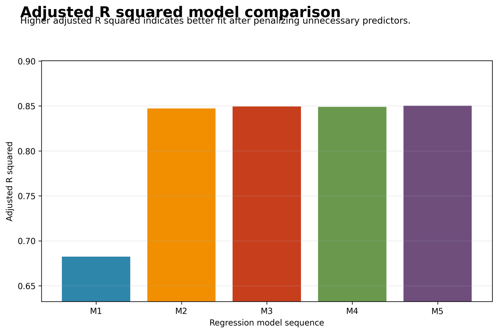
The first bar is much lower than the remaining bars because Model 1 uses only one prior-grade predictor and has adjusted R² of approximately .6824. Adding the second prior-grade measure raises adjusted R² to approximately .8473. Models 3, 4 and 5 cluster close to .85, showing diminishing improvements after the strong G1/G2 information is included.
The highest bar is Model 5 at approximately .8504. The visual difference between Models 3 and 5 is small, but Model 5 is still the adjusted-R² winner in the Python report. This corrects the tempting but inaccurate conclusion that the third bar must be highest simply because the models look nearly tied.
Chart 2: R Squared vs Adjusted R Squared
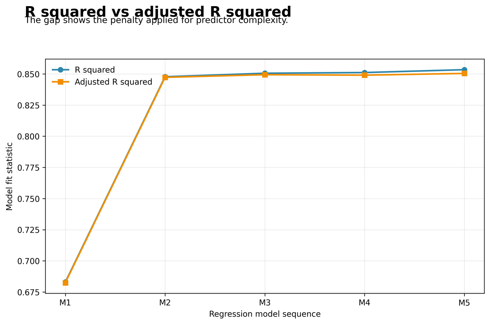
The two lines remain close because the sample is large relative to the model sizes. The gap is around .0005 for Models 1 and 2, .0012 for Model 3, .0021 for Model 4 and .0030 for Model 5. The widening distance illustrates the increasing complexity charge.
Raw R² rises at every step, from .6829 to .8534. Adjusted R² declines slightly from Model 3 to Model 4, then rises to its maximum in Model 5. The chart therefore shows both important behaviors: R² never punishes added predictors, while adjusted R² can move down or up depending on whether the new terms justify their cost.
Chart 3: Observed vs Predicted Final Model
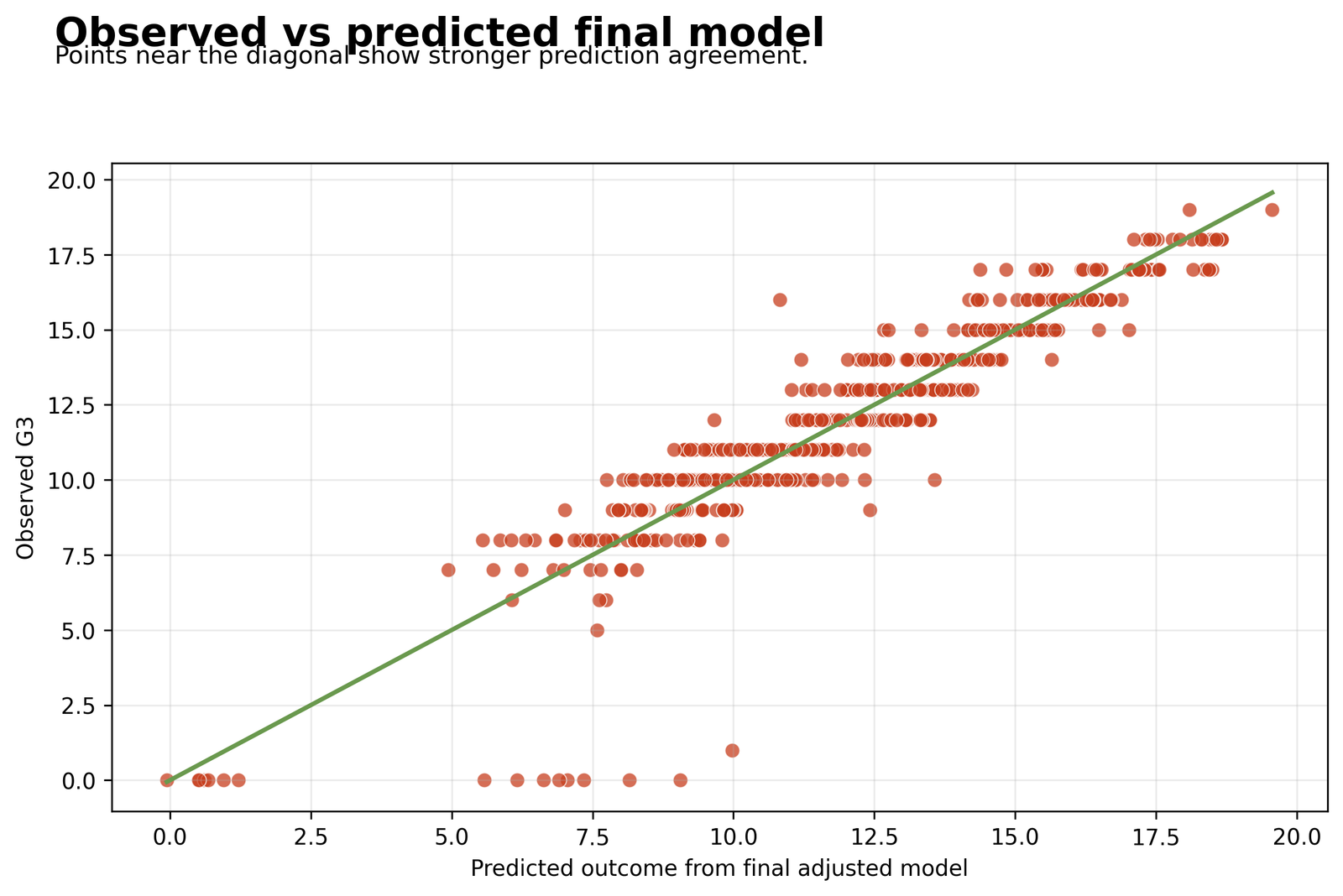
Most points lie close to the diagonal, especially across the middle and upper grade ranges, which is consistent with the strong R² and adjusted R². The horizontal bands occur because G3 is recorded as an integer grade while predictions are continuous. Points far below the diagonal indicate overprediction; points above it indicate underprediction.
Several observations with very low observed G3 sit well below their predicted values. These cases help explain the large negative residual tail. The chart supports strong overall agreement, but it also shows why a single fit statistic should not replace case-level diagnostic review.
Chart 4: Residuals vs Fitted Values
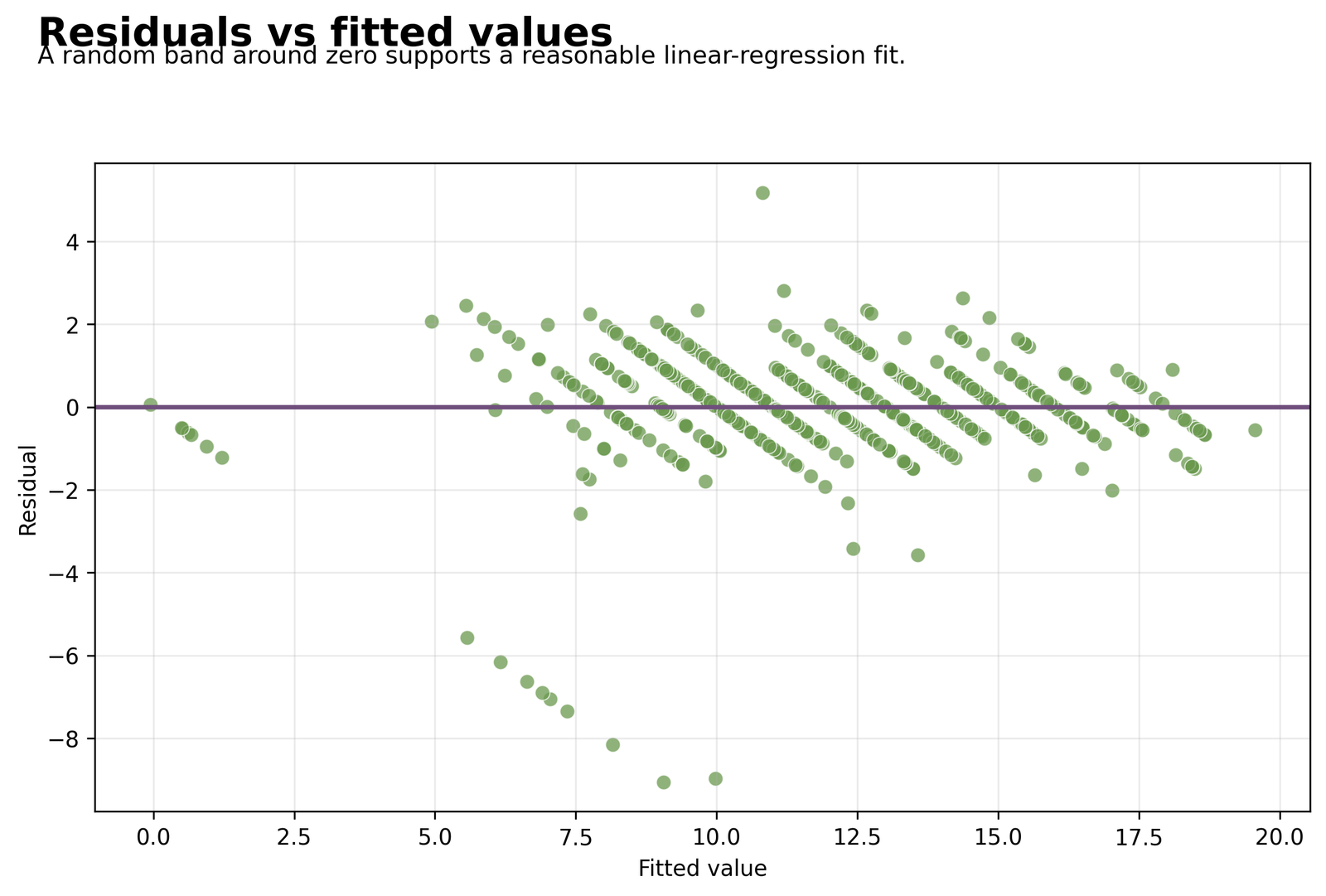
A residuals-versus-fitted plot should show errors scattered around zero without a strong curve or funnel. The supplied image includes positive and negative residuals around the zero line, but it also shows several large negative values. Those points require investigation because they may represent unusual outcomes, influential observations or model misspecification.
Media verification note: the text embedded in this uploaded image reads “ANOVA Residuals vs Fitted Values,” and its fitted values form only a few vertical bands. It should be treated as a general residual-diagnostic illustration. Before publishing, replace it with the adjusted-R² report-specific 04_residuals_vs_fitted.png if that file is uploaded later.
Chart 5: Standardized Residual Distribution
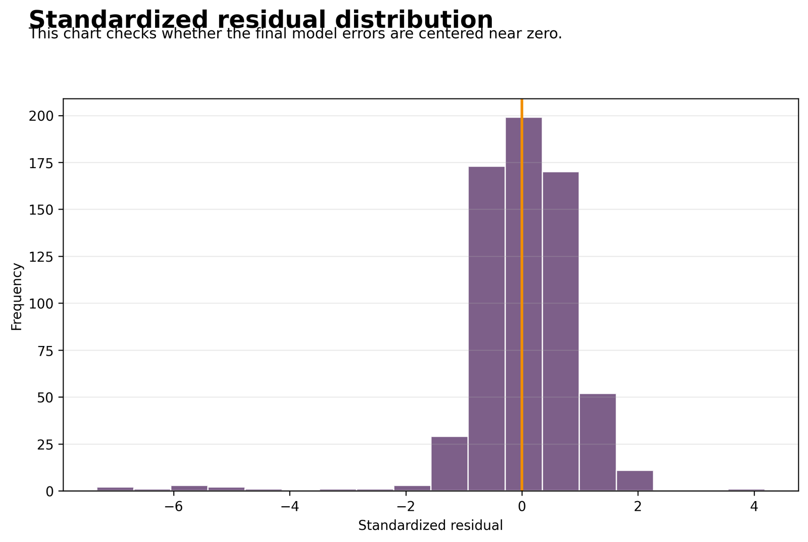
The histogram is concentrated near zero, but the left tail extends much farther than the right tail. SPSS reports standardized residuals from about -7.25 to 4.15, and its normality tests are significant. With n = 649, formal normality tests are sensitive, but the extreme left-tail cases are still practically important.
The appropriate conclusion is not that the model is unusable. Instead, report that the central residual mass is near zero while a small number of extreme observations create skewness and heavy tails. Use a Q-Q plot, P-P plot and outlier detection to identify the source of the departures.
Chart 6: Adjusted R Squared Complexity Penalty
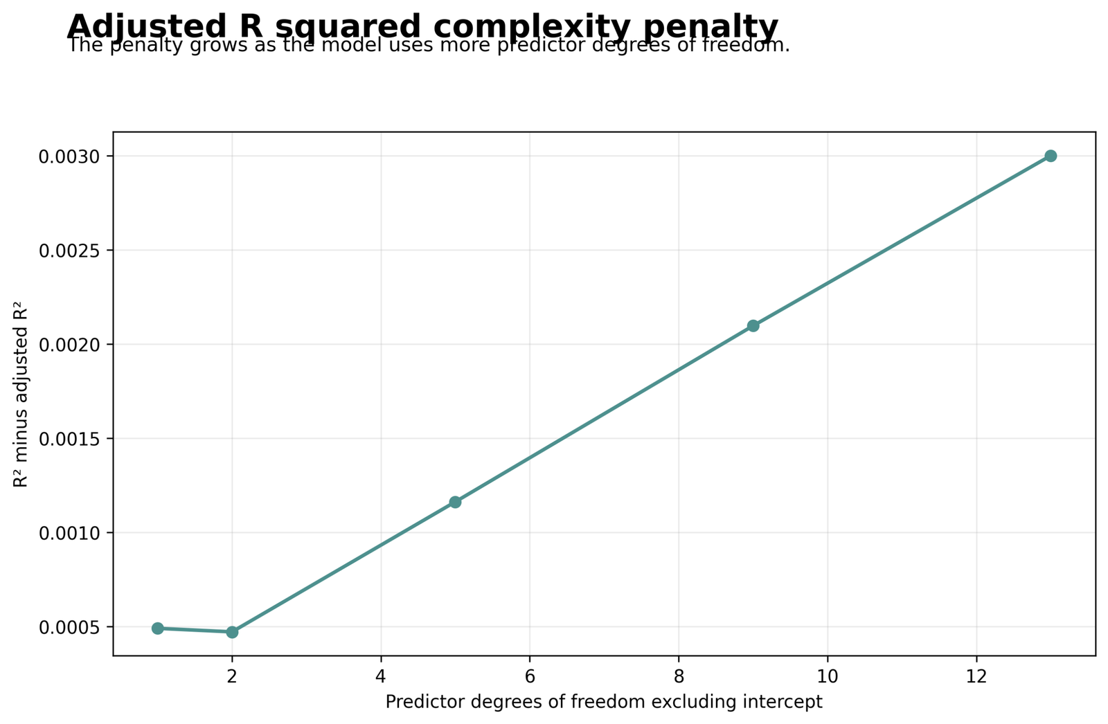
The penalty is smallest for the two-predictor model and grows as the model expands to 5, 9 and 13 predictor degrees of freedom. At 13 df, the gap is about .0030. The line is not a measure of overfitting by itself; it is the direct mathematical consequence of the adjusted R² formula combined with the observed R² improvements.
The final point remains small because the sample contains 649 observations. In a much smaller sample, the same 13-df model would receive a larger adjustment. This is why adjusted R² must always be interpreted with both n and p.
Chart 7: Top Coefficient t Values
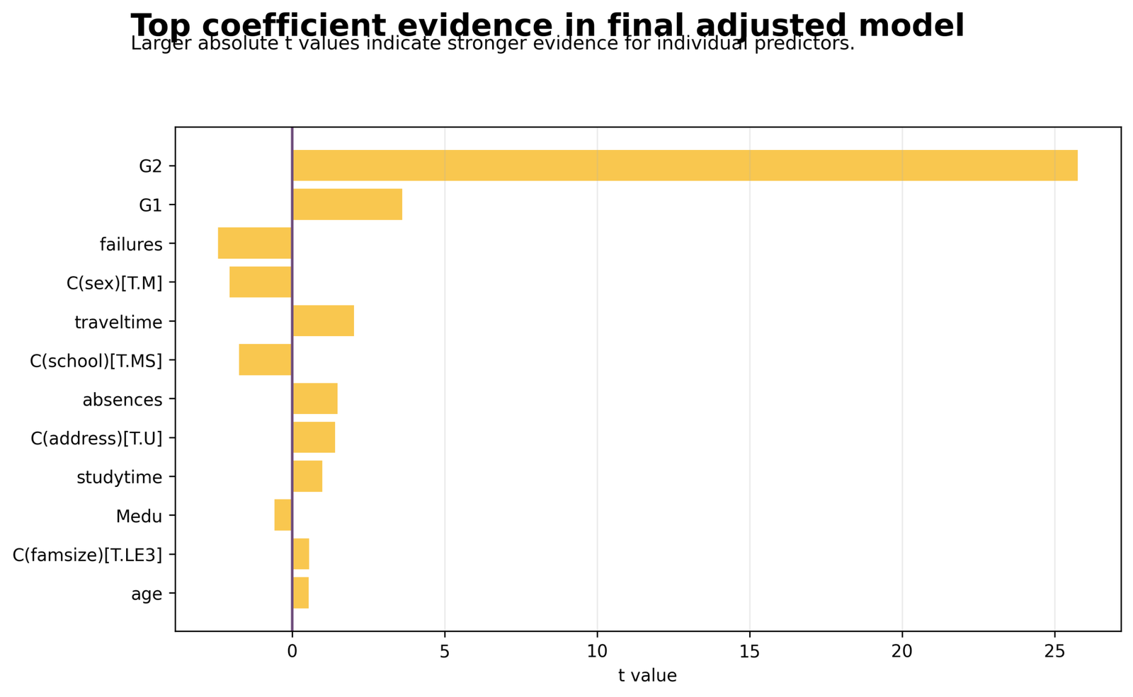
G2 dominates the chart with t approximately 25.76. G1 is a distant second at about 3.62. Failures and the male indicator have negative t values near -2.43 and -2.05, while traveltime is positive near 2.03. Most other predictors have absolute t values below 2.
The chart distinguishes overall model fit from individual evidence. The model can have adjusted R² above .85 even though many covariates are not individually significant, because the strong prior-grade variables explain most of the variation. Coefficient significance, effect size, multicollinearity and theoretical purpose should be assessed separately.
R Charts, Tables and Independent Validation
The R workflow fits the same five regression specifications with lm(), uses G3 as the outcome, and evaluates the models with R², adjusted R², RMSE, MAE, AIC and BIC. It reproduces the Python ranking: Model 5 has the highest adjusted R² and lowest in-sample RMSE and MAE, Model 3 has the lowest AIC, and Model 2 has the lowest BIC. The R report and chart discussion therefore provide software-to-software validation rather than a different statistical question.
R Model-Comparison Results
| R model | n | Predictor df | R² | Adjusted R² | Penalty | RMSE | MAE | AIC | BIC |
|---|---|---|---|---|---|---|---|---|---|
| Model 1: baseline prior grade | 649 | 1 | .6829 | .6824 | .0005 | 1.8178 | 1.2030 | 2621.4936 | 2630.4445 |
| Model 2: prior grade sequence | 649 | 2 | .8478 | .8473 | .0005 | 1.2596 | .7851 | 2147.3096 | 2160.7359 |
| Model 3: academic predictors | 649 | 5 | .8506 | .8494 | .0012 | 1.2479 | .7830 | 2141.2537 | 2168.1063 |
| Model 4: academic + demographics | 649 | 9 | .8511 | .8490 | .0021 | 1.2455 | .7788 | 2146.7840 | 2191.5384 |
| Model 5: full adjusted model | 649 | 13 | .8534 | .8504 | .0030 | 1.2359 | .7777 | 2144.6640 | 2207.3200 |
The consolidated R table prevents the chart section from becoming repetitive. Adjusted R² increases sharply from .6824 in Model 1 to .8473 in Model 2, reaches .8494 in Model 3, falls slightly to .8490 in Model 4, and then reaches the maximum of .8504 in Model 5. The final choice depends on the stated criterion: Model 5 for adjusted explained variance and in-sample error, Model 3 for AIC, or Model 2 for BIC.
Selected R Final-Model Coefficients
| Term | Coefficient | SE | t value | p-value | 95% CI | R interpretation |
|---|---|---|---|---|---|---|
| G2 | .8817 | .0342 | 25.7601 | <.001 | .8145 to .9489 | Dominant positive adjusted association with G3. |
| G1 | .1330 | .0368 | 3.6153 | .0003 | .0607 to .2052 | Positive independent association after controlling for the remaining terms. |
| failures | −.2313 | .0952 | −2.4308 | .0153 | −.4182 to −.0444 | Previous failures are associated with a lower fitted G3. |
| sex: M vs F | −.2165 | .1054 | −2.0534 | .0404 | −.4235 to −.0095 | The M-coded indicator is negative in the fully adjusted specification. |
| school: MS vs GP | −.2083 | .1199 | −1.7369 | .0829 | −.4437 to .0272 | The interval includes zero, so the adjusted school difference is not significant at .05. |
| address: U vs R | .1688 | .1195 | 1.4133 | .1580 | −.0657 to .4034 | No statistically reliable adjusted address effect. |
| studytime | .0630 | .0633 | .9952 | .3200 | −.0613 to .1872 | No statistically reliable adjusted study-time coefficient. |
| absences | .0167 | .0112 | 1.4944 | .1356 | −.0052 to .0386 | The small positive coefficient is not significant at .05. |
R Chart 1: Adjusted R Squared Model Comparison
The R validation chart begins with Model 1 adjusted R² = .6824, then rises to .8473 for Model 2. The large increase of approximately .1649 shows that adding the second prior-grade variable contributes far more explanatory information than the later model expansions. Model 3 reaches .8494, Model 4 records .8490, and Model 5 reaches the highest value of .8504.
The apparent near-tie among Models 3, 4 and 5 should be interpreted numerically. Model 4 is about .0004 lower than Model 3 because its additional terms do not fully overcome the larger predictor penalty. Model 5 then improves adjusted R² by about .0014 over Model 4 and by about .0010 over Model 3. R therefore confirms Model 5 as the adjusted-R² winner, although the practical gain beyond Model 3 is small.
R Chart 2: R Squared vs Adjusted R Squared
Ordinary R² rises monotonically from .6829 to .8478, .8506, .8511 and .8534. Adjusted R² follows the values .6824, .8473, .8494, .8490 and .8504. The two series are close because the sample size is 649, but the separation increases as the model consumes more predictor degrees of freedom.
The exact R²-minus-adjusted-R² penalties are approximately .0005, .0005, .0012, .0021 and .0030. The small fall in adjusted R² from Model 3 to Model 4 occurs even though raw R² increases from .8506 to .8511. This is the central reason for reporting adjusted R²: the additional Model 4 terms improve raw fit, but not enough to justify their full complexity cost.
R Chart 3: Observed vs Predicted G3 for the Final Model
The final R model uses 649 observations and 13 predictor degrees of freedom. Its R² = .8534, adjusted R² = .8504, RMSE = 1.2359 and MAE = .7777. Most fitted points lie near the 45-degree agreement line, especially through the central grade range, which is consistent with the model explaining more than 85% of sample variance.
The horizontal rows of points occur because the observed outcome G3 is recorded as an integer while fitted values are continuous. A small number of very low observed grades fall well below their fitted values, indicating overprediction and producing large negative residuals. The chart therefore supports strong aggregate fit but also identifies observations that should be investigated through studentized residuals, leverage and Cook’s distance.
R Chart 4: Residuals vs Fitted Values
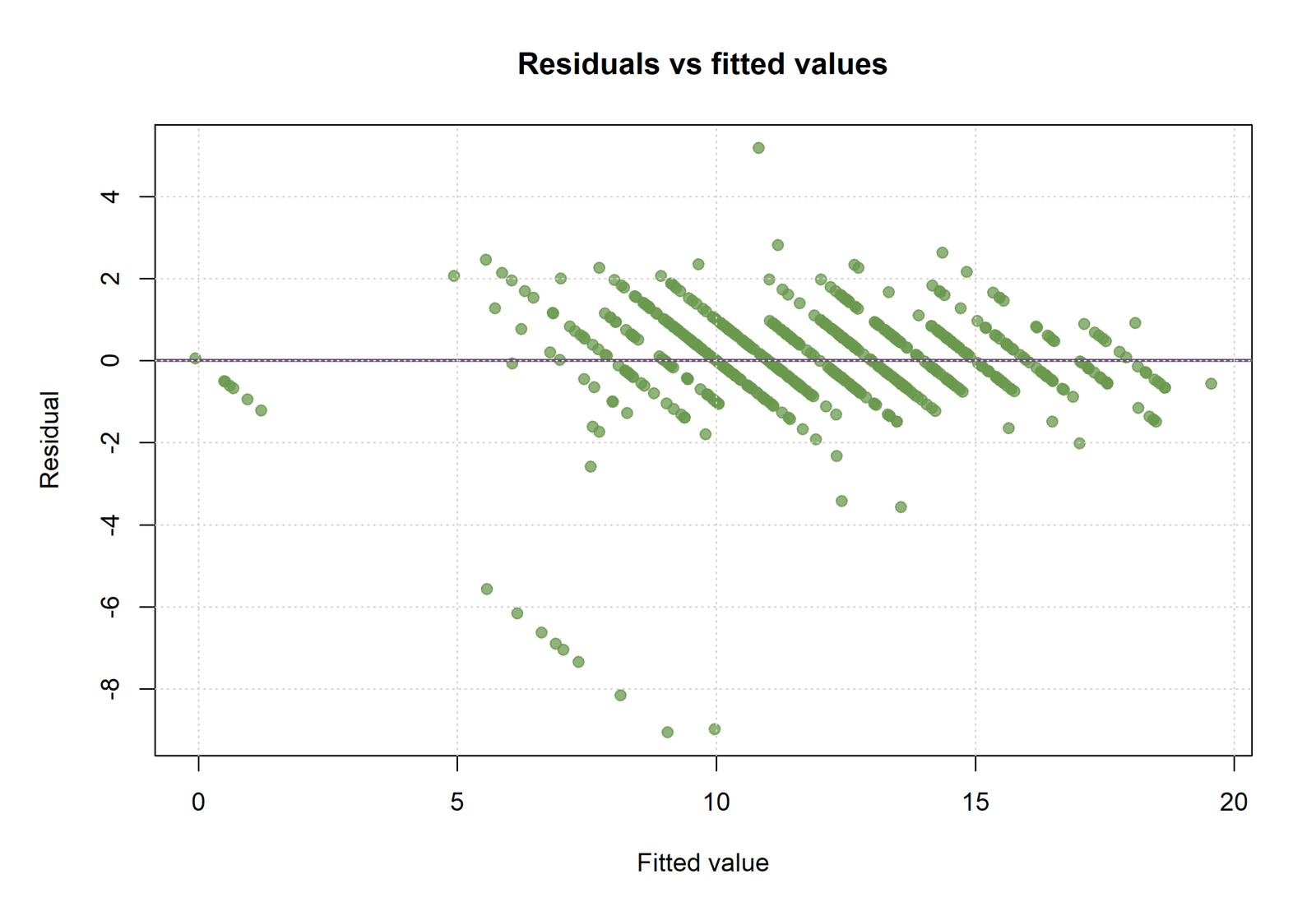
The residuals should fluctuate around zero without a systematic curve or progressively widening funnel. The output reports raw residuals from approximately −9.059 to 5.180. Most cases remain much closer to zero, but the long negative side shows that several low observed grades were predicted too highly by the final model.
Those extreme negative cases matter even though adjusted R² is .8504. Adjusted R² summarizes explained variation and does not test linearity, constant variance or influence. The R workflow should therefore pair this plot with formal or graphical checks for heteroskedasticity, nonlinear form and influential observations.
Supplied-media note: the embedded heading in this uploaded image identifies it as an ANOVA residual plot. It is retained because it is the residual-versus-fitted URL supplied for this post. Replace it with the report-specific R residual chart when that separate WordPress media URL is available.
R Chart 5: Standardized Residual Distribution
The standardized residuals range from approximately −7.250 to 4.146. The main body of the distribution is centered near zero, but the negative tail is longer and contains more extreme values than the positive tail. A perfectly normal residual distribution would be more symmetric and would rarely contain standardized residuals with absolute values this large.
The R interpretation should therefore separate central fit from tail behavior. Model 5 explains a large share of the variance, but a small group of cases departs strongly from the fitted relationship. A Q-Q plot, studentized residual review and influence analysis are necessary before claiming that the regression assumptions are fully satisfactory.
R Chart 6: Adjusted R Squared Complexity Penalty
The penalty is .000490 with one predictor degree of freedom, .000471 with two, .001162 with five, .0021 with nine, and .0030 with 13. The slight reduction from Model 1 to Model 2 occurs because the second predictor adds a very large amount of fit, while the larger later models receive progressively stronger adjustments.
The final .0030 penalty is still modest because n = 649 is large relative to 13 predictor degrees of freedom. This does not prove that the model is immune to overfitting. It means only that, under the adjusted-R² formula and this sample size, Model 5 retains most of its raw R² after the complexity correction.
R Chart 7: Top Final-Model Coefficient t Values
G2 dominates with t = 25.7601, followed by G1 with t = 3.6153. The strongest negative displayed terms are failures with t = −2.4308 and the M-coded sex indicator with t = −2.0534. The chart also places traveltime near a positive t value of about 2.03, while most remaining terms have absolute t values below 2.
This chart explains why a model can have adjusted R² = .8504 even when many individual terms are nonsignificant. G1 and especially G2 account for most of the strong fit. The other terms provide smaller incremental adjustments, possible confounding control or group comparisons. Overall adjusted fit, individual coefficient evidence and theoretical inclusion are related but distinct decisions.
R validation conclusion: R reproduces the same central result as Python and SPSS: Model 5 has R² = .8534 and adjusted R² = .8504, with F(13, 635) = 284.43 and p < .001. The model has strong in-sample explanatory fit, while residual extremes and the disagreement among adjusted R², AIC and BIC require a cautious, criterion-specific model-selection conclusion.
Regression Assumptions and Diagnostics
Adjusted R² is not an assumption test. A model can have high adjusted R² and still violate linearity, equal variance, independence, residual distribution or influence conditions. At minimum, examine residual plots, leverage, Cook’s distance and collinearity diagnostics.
| Diagnostic Question | Recommended Check | Why It Matters |
|---|---|---|
| Is the mean relationship approximately linear? | Observed-vs-predicted and residuals-vs-fitted plots. | Curvature means adjusted R² may summarize a misspecified linear model. |
| Is residual variance reasonably stable? | Breusch-Pagan test or White test. | Heteroskedasticity affects standard errors and inference. |
| Are predictors excessively redundant? | VIF, tolerance and the multicollinearity guide. | Strong collinearity can destabilize coefficients even when fit is high. |
| Are individual cases unusually influential? | Cook’s distance, leverage and studentized residuals. | A few cases can drive coefficients and fit statistics. |
| Is the functional form incomplete? | Ramsey RESET plus theory-based nonlinear terms. | Omitted nonlinear structure can reduce interpretability. |
The SPSS output shows a maximum Cook’s distance of approximately .140, which is not automatically decisive but is far above the median and deserves case review. The extreme standardized residuals are more immediately visible. Report diagnostic findings rather than hiding them behind the high adjusted R².
Adjusted R Squared, AIC, BIC and Predictive Performance
Adjusted R² is one model-selection criterion, not the only criterion. In the Python table, adjusted R² chooses Model 5, AIC chooses Model 3 and BIC chooses Model 2. This disagreement is informative. Model 5 has the best in-sample adjusted fit and error metrics, but Model 2 or Model 3 may be preferred when parsimony is more important.
| Criterion | Preferred Python Model | Interpretation |
|---|---|---|
| Highest adjusted R² | Model 5 | Best penalized explained variance in this sample. |
| Lowest RMSE / MAE | Model 5 | Lowest in-sample prediction error among the five models. |
| Lowest AIC | Model 3 | Best likelihood-complexity tradeoff under the AIC penalty. |
| Lowest BIC | Model 2 | Best under the stronger BIC complexity penalty. |
For prediction, use cross-validation, a holdout test set or predicted R². Adjusted R² is calculated from the training sample and can still look optimistic when the analyst repeatedly searches many models. Model selection should combine theory, pre-specified goals, diagnostic quality and out-of-sample evidence.
SPSS, Python, R and Excel Workflows
| Software | Main Workflow | Best Use |
|---|---|---|
| SPSS | Prepare dummy variables, run Linear Regression for each candidate model, read Model Summary and ANOVA tables, save residuals and influence statistics. | Formal output, classroom interpretation and thesis appendices. |
| Python | Fit formulas with statsmodels, extract rsquared_adj, compare AIC/BIC/RMSE/MAE, save charts and a PDF report. | Reproducible automation and publication-ready charts. |
| R | Fit lm() models, read summary(model)$adj.r.squared, compare AIC/BIC and inspect diagnostic plots. | Compact statistical validation and extensible modeling. |
| Excel | Calculate predictions, residuals, SSE, SST, R² and adjusted R² with visible formulas. | Formula teaching and transparent worked calculations. |
Code Blocks for Adjusted R Squared
SPSS Syntax
* Adjusted R Squared final model in SPSS.
* Assumes the variables are already open and categorical dummies are prepared.

SET PRINTBACK=OFF MPRINT=OFF RESULTS=ON DECIMAL=DOT.
OUTPUT CLOSE ALL.
OUTPUT NEW NAME=AdjustedRSquaredOutput.

REGRESSION
  /DEPENDENT G3
  /METHOD=ENTER G1 G2 studytime failures absences age Medu Fedu traveltime
                school_dummy sex_dummy address_dummy famsize_dummy
  /STATISTICS COEFF OUTS R ANOVA CHANGE COLLIN TOL CI(95)
  /RESIDUALS HISTOGRAM(ZRESID) NORMPROB(ZRESID)
  /SAVE PRED ZPRED RESID ZRESID COOK LEVER.

OUTPUT SAVE OUTFILE='D:\DATA ANALYSIS\H Regression Tests and Models\Adjusted R Squared\SPSS_Output\spv\Adjusted-R-Squared-Output.spv'.
OUTPUT EXPORT
  /CONTENTS EXPORT=ALL LAYERS=PRINTSETTING MODELVIEWS=PRINTSETTING
  /PDF DOCUMENTFILE='D:\DATA ANALYSIS\H Regression Tests and Models\Adjusted R Squared\SPSS_Output\pdf\Adjusted-R-Squared-SPSS-Output.pdf'.
Python Code
import numpy as np
import pandas as pd
import statsmodels.formula.api as smf
from sklearn.metrics import mean_absolute_error, mean_squared_error

DATA_FILE = "dataset.csv"
df = pd.read_csv(DATA_FILE)

formula = (
    "G3 ~ G1 + G2 + studytime + failures + absences + age + "
    "Medu + Fedu + traveltime + C(school) + C(sex) + "
    "C(address) + C(famsize)"
)
model = smf.ols(formula, data=df).fit()

pred = model.predict(df)
valid = model.model.data.row_labels
observed = df.loc[valid, "G3"].astype(float)
predicted = pd.Series(pred, index=valid)

rmse = np.sqrt(mean_squared_error(observed, predicted))
mae = mean_absolute_error(observed, predicted)

print("R squared:", model.rsquared)
print("Adjusted R squared:", model.rsquared_adj)
print("F statistic:", model.fvalue)
print("F-test p-value:", model.f_pvalue)
print("AIC:", model.aic, "BIC:", model.bic)
print("RMSE:", rmse, "MAE:", mae)
print(model.summary())
R Code and R Report PDF
The R report contains the R model summary, adjusted R-squared calculations, coefficient output, model-comparison results and regression diagnostic charts generated by the R workflow.
df <- read.csv("dataset.csv", stringsAsFactors = TRUE)

model5 <- lm(
  G3 ~ G1 + G2 + studytime + failures + absences + age +
    Medu + Fedu + traveltime + school + sex + address + famsize,
  data = df
)

s <- summary(model5)
cat("R squared:", s$r.squared, "
")
cat("Adjusted R squared:", s$adj.r.squared, "
")
cat("AIC:", AIC(model5), "
")
cat("BIC:", BIC(model5), "
")

pred <- fitted(model5)
res <- residuals(model5)
rmse <- sqrt(mean(res^2))
mae <- mean(abs(res))
cat("RMSE:", rmse, "MAE:", mae, "
")

par(mfrow = c(2, 2))
plot(model5)
Excel Formulas
Assume:
Observed G3 range = L2:L650
Predicted G3 range = M2:M650
Residual range = N2:N650
Squared residual range = O2:O650
Squared deviation range = P2:P650

Residual:
=L2-M2

Squared residual:
=N2^2

Squared deviation from outcome mean:
=(L2-AVERAGE($L$2:$L$650))^2

SSE:
=SUM(O2:O650)

SST:
=SUM(P2:P650)

R squared:
=1-(SSE/SST)

Adjusted R squared:
=1-(1-R_squared)*(n-1)/(n-p-1)

RMSE using n:
=SQRT(SSE/n)

Regression standard error using residual df:
=SQRT(SSE/(n-p-1))
APA-Style Reporting for Adjusted R Squared
Full Python/SPSS Model Report
A multiple linear regression model was fitted to predict G3 final grade from nine numeric predictors and four categorical predictor terms. The analysis included 649 complete observations and 13 predictor degrees of freedom. The overall model was statistically significant, F(13, 635) = 284.43, p < .001. The model explained 85.34% of the sample variance in G3, R² = .853, and retained an adjusted R² of .850 after the complexity correction. The Python RMSE was 1.236 and MAE was .778. G2 was the strongest positive predictor, B = .882, t = 25.76, p < .001, followed by G1, B = .133, t = 3.62, p < .001. Previous failures had a negative adjusted association with G3, B = −.231, t = −2.43, p = .015.
Model Comparison Report
Five regression models were compared using adjusted R². Adjusted R² increased from .6824 in the one-predictor baseline model to .8473 in the two-prior-grade model, .8494 in the five-predictor academic model, .8490 in the nine-df academic-demographic model and .8504 in the 13-df full model. Model 5 had the highest adjusted R² and the lowest in-sample RMSE, whereas Model 3 had the lowest AIC and Model 2 had the lowest BIC. Model choice therefore depended on whether the priority was adjusted explained variance, prediction error or parsimony.
R Validation Report
The R regression sequence reproduced the five-model comparison obtained in Python. For the final 13-df model, R² = .8534 and adjusted R² = .8504, with RMSE = 1.2359 and MAE = .7777. Model 5 had the highest adjusted R², Model 3 had the lowest AIC, and Model 2 had the lowest BIC. The strongest coefficient evidence was observed for G2, B = .8817, t = 25.7601, p < .001, followed by G1, B = .1330, t = 3.6153, p = .0003.
Excel Worked-Model Report
In the separate 10-predictor Excel worked model, n = 649, R² = .8516 and adjusted R² = .8493. The adjustment penalty was .0023, RMSE was 1.243 and MAE was .778. Within the workbook's numeric-model sequence, Model 3 had the highest adjusted R², .8494, narrowly exceeding the full numeric Model 5.
Common Mistakes When Interpreting Adjusted R Squared
| Mistake | Why It Is Wrong | Better Practice |
|---|---|---|
| Calling adjusted R² “model accuracy” | It measures adjusted explained variation, not the percentage of exact predictions. | Report RMSE, MAE and test-sample performance for predictive accuracy. |
| Comparing models with different samples | Changed missing-data cases can alter SST and make the values non-comparable. | Use the same outcome and same observations. |
| Counting categorical variables as one predictor | Multi-level factors may consume several degrees of freedom. | Use predictor df excluding the intercept. |
| Assuming the highest adjusted R² is automatically final | AIC, BIC, theory and validation may prefer a simpler model. | State the selection criterion and compare alternatives. |
| Ignoring residual diagnostics | High adjusted R² can coexist with outliers, heteroskedasticity or nonlinearity. | Inspect residuals, influence and collinearity. |
| Mixing Excel and Python/SPSS values | The supplied outputs use different predictor specifications. | Label the 10-predictor workbook and 13-df Python/SPSS model separately. |
| Reporting excessive decimals | Long machine precision distracts from interpretation. | Use three decimals in narrative reporting and retain more only in reproducibility tables. |
Downloads and Resources
FAQs About Adjusted R Squared
What does adjusted R squared mean?
It is the proportion of sample outcome variation explained by a regression model after a penalty based on sample size and predictor degrees of freedom. In the main Python model, adjusted R² = .8504.
What is the difference between R squared and adjusted R squared?
R² never decreases when predictors are added to a standard intercept model. Adjusted R² can decrease when a new predictor does not improve fit enough to justify its additional degree of freedom.
How do you calculate adjusted R squared?
Use 1 − (1 − R²)(n − 1)/(n − p − 1), where n is the number of observations and p is the predictor degrees of freedom excluding the intercept.
Can adjusted R squared be negative?
Yes. A negative value means the fitted predictors perform worse than the intercept-only benchmark after the complexity adjustment.
Is adjusted R squared always smaller than R squared?
For a conventional OLS model with an intercept and the standard definitions, adjusted R² is less than or equal to R². Unconventional no-intercept definitions can behave differently.
Can adjusted R squared increase when a variable is added?
Yes. It increases when the added predictor reduces unexplained variation enough to overcome the penalty. In the Python sequence, adjusted R² rises from Model 4 to Model 5.
What is a good adjusted R squared value?
There is no universal threshold. A good value depends on the outcome, field, noise level, measurement reliability and intended use. Compare it with justified benchmark models.
Should I report R squared or adjusted R squared?
For multiple regression, report both. R² describes unadjusted sample fit, while adjusted R² communicates the complexity-corrected fit.
Why do the Excel and Python values differ in this guide?
The Excel workbook uses a 10-numeric-predictor teaching model. The Python and SPSS outputs use a broader 13-df model with categorical indicators. Always compare figures within the same specification.
Does a high adjusted R squared prove the model assumptions are met?
No. Residual shape, equal variance, linearity, influence, independence and collinearity must be checked separately.
Is adjusted R squared enough for model selection?
No. Consider AIC, BIC, theory, residual diagnostics and out-of-sample validation. In this example, adjusted R², AIC and BIC select different models.
How should adjusted R squared be reported in APA style?
State the outcome, predictors or predictor df, sample size, R², adjusted R², F statistic with degrees of freedom, p value and an error metric such as RMSE.

