
Krippendorff’s Alpha: 7 Essential Steps, Formula and Worked Example
The Krippendorff’s Alpha coefficient measures agreement by comparing observed disagreement with disagreement expected from pooled category values. This complete nominal example uses three categorized grade occasions for 649 students and explains the formula, coincidence matrix, interpretation, assumptions, Python, R, SPSS and Excel workflows.
Nominal categories
649 subjects
Missing-data capable method
Python + R + SPSS + Excel
Agreement exceeded chance expectation, but the result did not reach the common tentative-reliability threshold.
In this worked Krippendorff’s Alpha example, categorized first-period, second-period and final grades were treated as three nominal rating occasions for 649 students. The exact result was Krippendorff’s Alpha = 0.642309, with observed disagreement = 0.215716 and expected disagreement = 0.603081. The coefficient shows meaningful consistency, yet it is below the frequently cited 0.667 boundary for tentative conclusions and below the 0.800 level often preferred for dependable reliability.
What does Krippendorff’s Alpha measure?
A chance-corrected reduction in disagreement, not a general association coefficient.
Krippendorff’s Alpha is a general reliability coefficient for values assigned to the same units by two or more coders, raters, judges, instruments, algorithms or repeated procedures. It answers a disagreement question rather than a correlation question: how much smaller is the observed disagreement within units than the disagreement expected from the pooled values?
The reliability question
The method begins with units that receive multiple values. In content analysis, the units may be documents and the sources may be coders. In clinical research, the units may be patients and the sources may be clinicians. In machine-learning annotation, the units may be images and the sources may be annotators. The worked analysis uses students as units and categorized G1, G2 and G3 grades as the three rating occasions.
Unlike raw agreement, Krippendorff’s Alpha adjusts for the disagreement expected from the observed category prevalence. A category used very often will generate some matches even when values are not reliably assigned. The expected-disagreement term prevents those predictable matches from receiving full credit.
What the coefficient is not
The coefficient is not an ordinary correlation. Two rating sources can be highly correlated while one systematically assigns higher values. It is also not a measure of internal consistency among questionnaire items, so it should not be substituted for Cronbach’s Alpha or Guttman’s Lambda.
The statistic is not the raw percentage of subjects with complete agreement. In this example, 67.64% of students have the same category on all three occasions, whereas Krippendorff’s Alpha = 0.642309. These numbers answer different questions.
The method is unusually broad because disagreement can be defined for nominal, ordinal, interval, ratio or custom-valued data. Nominal Krippendorff’s Alpha assigns the same penalty to every mismatch. Ordinal alpha gives greater penalty to more distant ordered categories. Interval and ratio forms use numerical distances. The scale-level choice is part of the statistical model and must be stated in the report.
When should you use Krippendorff’s Alpha?
Use the decision logic below before selecting software or interpreting a coefficient.
Use Krippendorff’s Alpha when the same units receive at least two pairable values and the research objective concerns reliability, reproducibility or agreement. The method is especially useful when the number of ratings varies across units, missing ratings occur, more than two sources are involved or the measurement level requires a distance function other than simple exact matching.
Define units
State what every row or case represents.
Define sources
Name coders, occasions, devices or algorithms.
Choose the scale
Nominal, ordinal, interval, ratio or custom.
Check pairability
Each contributing unit needs at least two usable values.
Set a standard
Choose the minimum acceptable reliability before interpretation.
Good uses
Do not use it automatically
In the worked dataset, using G1, G2 and G3 as sources is statistically possible but substantively unusual. These columns are repeated grade occasions, not independent human judges. The interpretation is therefore stability of grade-band classification across time. If the objective were numerical test-retest reliability on the original 0-to-20 scores, test-retest reliability or an agreement model for continuous values could be more informative.
Krippendorff’s Alpha assumptions: six conditions to check
The method is flexible, but a reliable conclusion still depends on design validity.
The main Krippendorff’s Alpha assumptions concern the design and meaning of the ratings rather than normality or equal variances. The method can be calculated for many data structures, but a valid reliability conclusion still requires coherent units, common category definitions, an appropriate distance function and transparent missing-data handling.
Identifiable units
Every set of ratings must belong to a clearly defined unit. Values from different students, documents or cases must not be accidentally combined.
Comparable sources
All sources must apply the same value system. A category labeled “high” must have the same operational meaning in every column.
Suitable measurement level
The selected disagreement function must match the scale. Nominal alpha treats every unequal pair alike; ordinal alpha preserves order.
Independent rating process
Human raters should normally work without seeing one another’s judgments. Dependence changes the reliability interpretation.
Pairable values
A contributing unit needs at least two usable ratings. Units with zero or one usable value contain no agreement information.
Representative units
The sampled units should represent the population and difficulty range to which the reliability conclusion will be generalized.
Krippendorff’s Alpha does not require normally distributed ratings. It does not require equal group variances. It does not require the same number of ratings for every unit. Those advantages are important, yet they should not be summarized as “assumption free.” A reliability statistic cannot compensate for unclear categories, dependent coding, unrepresentative units or a distance function that contradicts the substantive decision.
The worked data contain 649 complete rows and no missing G1, G2 or G3 values. Every student contributes three ratings and three unordered within-student pairs. Category prevalence is not extreme enough to make any category absent, but the middle category is dominant and no low-high disagreement occurs. Those features should be reported because they shape expected disagreement and the range of disagreements represented by the sample.
Krippendorff’s Alpha hypotheses: observed versus expected disagreement
The mathematical null is chance-level agreement, while the practical null may be failure to reach a required minimum.
The null hypothesis for nominal Krippendorff’s Alpha states that observed disagreement within units is equal to the disagreement expected when the pooled values are paired without preserving unit membership. The alternative states that observed disagreement is smaller, producing reliability above chance expectation.
Formal disagreement hypotheses
Under the chance model, within-unit values are no more similar than pooled values paired without regard to their original units.
Within-unit values disagree less than expected, indicating agreement beyond the pooled-value baseline.
Negative alpha values occur when Do exceeds De. Such a result indicates systematic disagreement greater than expected and should trigger a review of reversed coding, incompatible rules or source drift.
Applied variables in this analysis
The same thresholds are applied to every occasion. Python and R may code the labels as 0, 1 and 2, while SPSS displays 1, 2 and 3. The numeric label shift does not change nominal alpha.
Reliability threshold hypothesis versus zero-agreement hypothesis
Testing whether alpha is greater than zero is often less useful than evaluating whether the coefficient reaches a prespecified reliability standard. A coefficient can be clearly above zero and still be too low for dependable coding. The worked value, 0.642309, demonstrates meaningful agreement beyond expectation but remains below the commonly cited 0.667 tentative boundary.
A practical reliability decision can be written as H0: α ≤ αmin versus H1: α > αmin, where αmin is chosen from the consequences of disagreement. A bootstrap confidence interval is usually more informative for this decision than a simple test against zero.
Krippendorff’s Alpha formula, coincidence matrix and hand calculation
Observed disagreement is divided by expected disagreement and subtracted from one.
The Krippendorff’s Alpha formula is short, but the coincidence structure behind it is the key to correct calculation. Nominal alpha uses zero disagreement for equal categories and one disagreement for unequal categories, then compares observed within-unit disagreement with the expected disagreement derived from pooled category frequencies.
Step 1: calculate observed disagreement
Do is the average disagreement among values assigned to the same units. De is the disagreement expected from the pooled distribution.
Each complete three-rating unit supplies three unordered pairs: G1–G2, G1–G3 and G2–G3. A unanimous pattern contributes zero disagreement. A two-versus-one pattern contributes two disagreeing pairs and one agreeing pair, so its subject disagreement is 2/3. The dataset contains 439 unanimous students and 210 two-versus-one students.
The equivalent pair calculation is 420 discordant pairs divided by 1,947 total within-unit pairs.
Step 2: calculate expected disagreement from pooled values
The pooled frequencies are 402 low, 1,047 middle and 498 high ratings, giving 1,947 total values. For nominal data under finite-sample pairing without replacement:
nc is the pooled count for category c and n is the total number of pairable values.
Step 3: substitute the two disagreement components
Observed disagreement is approximately 35.77% of expected disagreement. Krippendorff’s Alpha is the complementary 64.23% reduction in expected disagreement.
Observed nominal coincidence matrix
| Observed coincidence | Low | Middle | High | Row total |
|---|---|---|---|---|
| Low | 284 | 118 | 0 | 402 |
| Middle | 118 | 837 | 92 | 1,047 |
| High | 0 | 92 | 406 | 498 |
| Column total | 402 | 1,047 | 498 | 1,947 |
The diagonal total is 1,527 and the off-diagonal total is 420. The matrix is symmetric because every pair contributes in both directions within the coincidence representation. Its row and column totals reproduce the pooled category counts, providing an important calculation check.
Krippendorff’s Alpha example: three categorized grade occasions
A complete 649-subject example with transparent coding, counts and pattern frequencies.
This Krippendorff’s Alpha example uses 649 students with three complete grade occasions. G1, G2 and G3 are originally scored from 0 to 20 and are recoded into low, middle and high categories using identical cut points. The worked analysis therefore measures exact grade-band stability rather than numerical score agreement.
Research scenario
The question is whether students remain in the same broad performance band across G1, G2 and G3 more consistently than expected from the overall category distribution. Each student is a unit and each grade occasion is treated as a rating source.
The temporal design means some mismatch may represent genuine learning or performance change. The result is therefore interpreted as category stability, not as independent-coder compliance.
Variables used
| Role | Variable | Coding / meaning |
|---|---|---|
| Unit | Student row | One student receiving three grade classifications. |
| Source 1 | G1 | First-period grade recoded to low, middle or high. |
| Source 2 | G2 | Second-period grade recoded with identical thresholds. |
| Source 3 | G3 | Final grade recoded with identical thresholds. |
| Distance | Nominal | 0 for equal categories; 1 for unequal categories. |
The final occasion contains fewer low classifications and more high classifications than the first occasion. G1 has 157 low and 152 high students, while G3 has 100 low and 194 high students. The middle category remains dominant. This directional shift explains why agreement should be discussed beside the category frequencies rather than reduced to one coefficient.
| Pattern | Frequency | Percent | Agreement interpretation |
|---|---|---|---|
| Middle–middle–middle | 235 | 36.21% | Complete agreement |
| High–high–high | 124 | 19.11% | Complete agreement |
| Low–low–low | 80 | 12.33% | Complete agreement |
| Low–middle–middle | 42 | 6.47% | G1 differs; G2 and G3 agree |
| Middle–middle–high | 36 | 5.55% | Final occasion moves upward |
| Middle–low–middle | 29 | 4.47% | Temporary G2 decline |
| Low–low–middle | 27 | 4.16% | Final occasion moves upward |
| Middle–high–high | 25 | 3.85% | Later occasions agree |
| Other two-versus-one patterns | 51 | 7.86% | One source differs from the other two |
No student has a low-high mismatch. Every observed disagreement occurs between adjacent grade bands. Nominal Krippendorff’s Alpha still assigns every mismatch the same penalty. An ordinal sensitivity analysis would recognize the ordered category structure and would answer a different, less strict agreement question.
Krippendorff’s Alpha statistics, results and interpretation
All four analysis artifacts reconcile to the same nominal coefficient and disagreement components.
The exact Krippendorff’s Alpha results reconcile across the Python report, R report, SPSS output ledger and worked Excel workbook. The coefficient is derived from 420 discordant pairs among 1,947 within-subject pair comparisons and from the pooled category prevalence used to calculate expected disagreement.
Primary reliability result
Below the common 0.667 tentative boundary
Observed disagreement is substantially smaller than expected disagreement, but the reduction is not large enough for dependable reliability under the commonly cited convention.
Calculation audit
| Evidence source | Key result | Supporting values | Interpretation |
|---|---|---|---|
| Python report | α = 0.642309 | Dₒ = 0.215716; Dₑ = 0.603081 | Nominal agreement beyond expectation |
| R report | α = 0.642309 | Three sources; 649 units | Independent cross-platform confirmation |
| SPSS output | Pairwise κ = .634 and .591 shown; alpha ledger = .642309 | 649 valid cases; zero missing | Descriptive and pairwise validation plus checked alpha |
| Excel workbook | α = 0.642309 | Absolute differences effectively zero | Formula-driven reconstruction and audit |
The SPSS crosstabs show G1–G2 Cohen’s Kappa = .634 and G1–G3 Cohen’s Kappa = .591, both displayed with p = .000 in SPSS. Those displayed values should be written as p < .001. A reconstructed G2–G3 table gives Cohen’s Kappa ≈ .704. These pairwise coefficients are diagnostics, not substitutes for the pooled three-source Krippendorff’s Alpha.
Pairwise exact agreement is 77.81% for G1–G2, 75.19% for G1–G3 and 82.28% for G2–G3. Upward transitions outnumber downward transitions, especially from G1 to G3. This pattern is consistent with a temporal improvement in grade categories rather than arbitrary coding disagreement.
Krippendorff’s Alpha in Python: calculation and charts
The first chart is full width; the remaining four charts are displayed in paired rows exactly as in the supplied format.
A dependable Krippendorff’s Alpha Python workflow verifies the raw dimensions, applies identical category thresholds, orients the matrix correctly and checks observed and expected disagreement rather than accepting a single package output without an audit trail.
import pandas as pddf = pd.read_csv("dataset.csv")
ratings = df[["G1", "G2", "G3"]].copy()
ratings = ratings.apply(lambda s: pd.cut(
s, bins=[-1, 9, 13, 20], labels=[0, 1, 2]
).astype(int))
# ratings.T is 3 sources × 649 units.
# Use a validated alpha function with level_of_measurement="nominal".
# Independently verify Do, De, and alpha = 1 - Do / De.
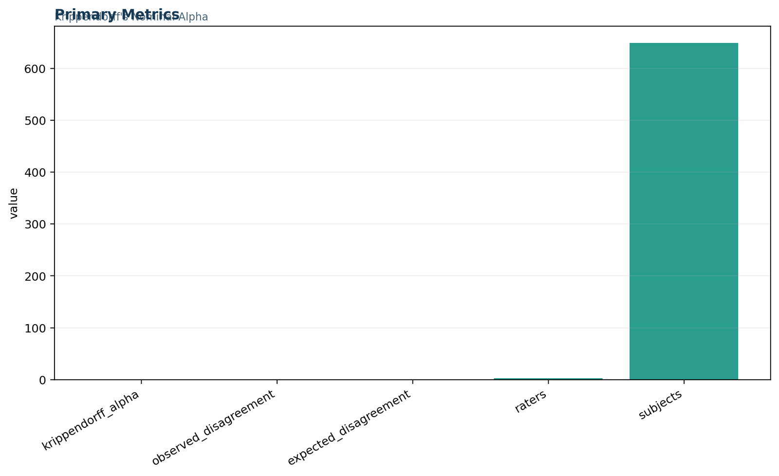
Python result summary
The primary-metrics chart reports Krippendorff’s Alpha = 0.642309, observed disagreement = 0.215716, expected disagreement = 0.603081, three rating occasions and 649 subjects. Because counts and proportions use different units, the exact labels are more informative than relative bar height.
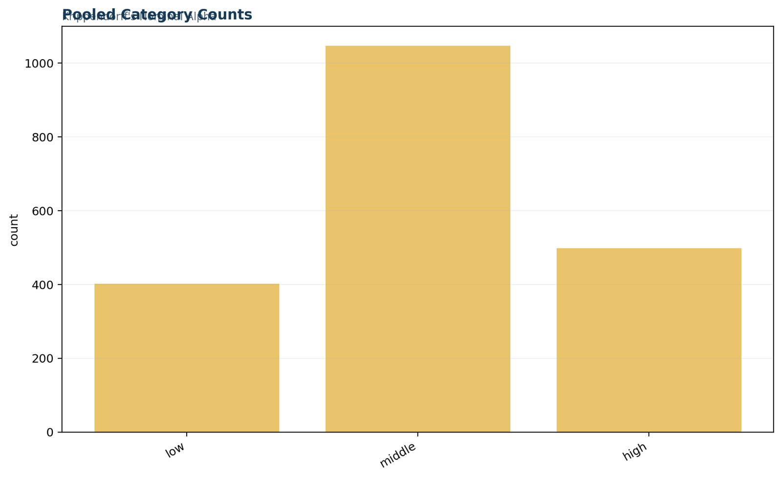
Python pooled category counts
The pooled ratings contain 402 low, 1,047 middle and 498 high classifications. The middle category accounts for 53.78% of all values and therefore contributes substantial chance agreement to the expected-disagreement model.
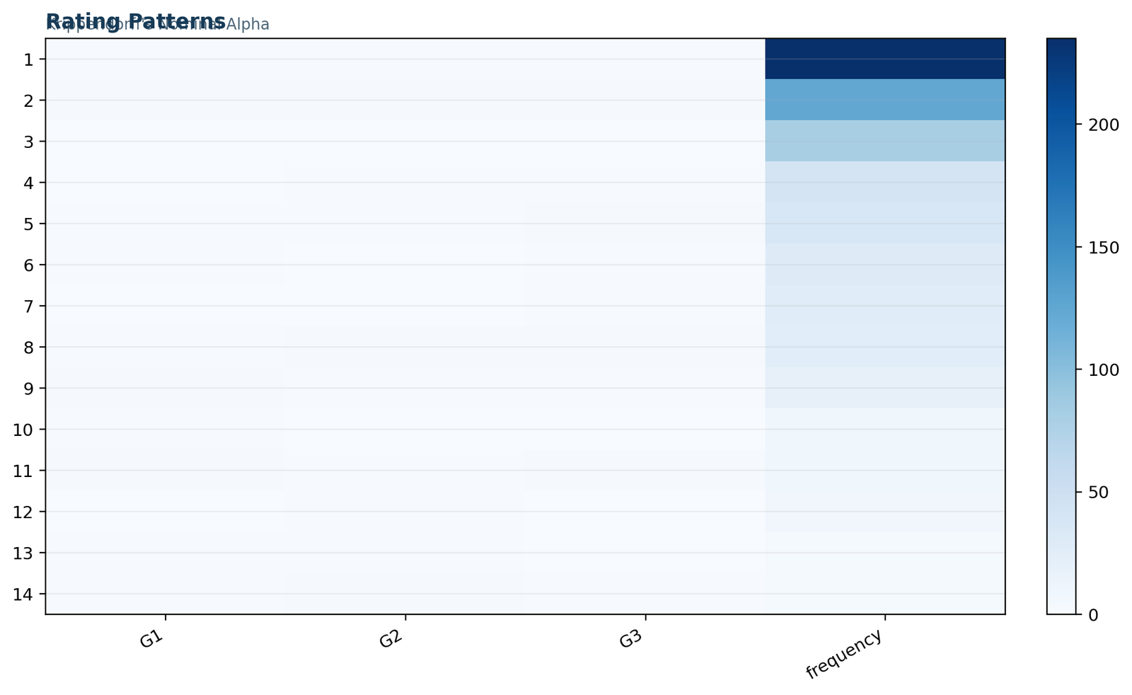
Python rating-pattern frequencies
The pattern chart summarizes the observed three-occasion configurations. Complete middle agreement is most frequent at 235 students, followed by complete high agreement at 124 and complete low agreement at 80. The remaining patterns are all two-versus-one configurations.
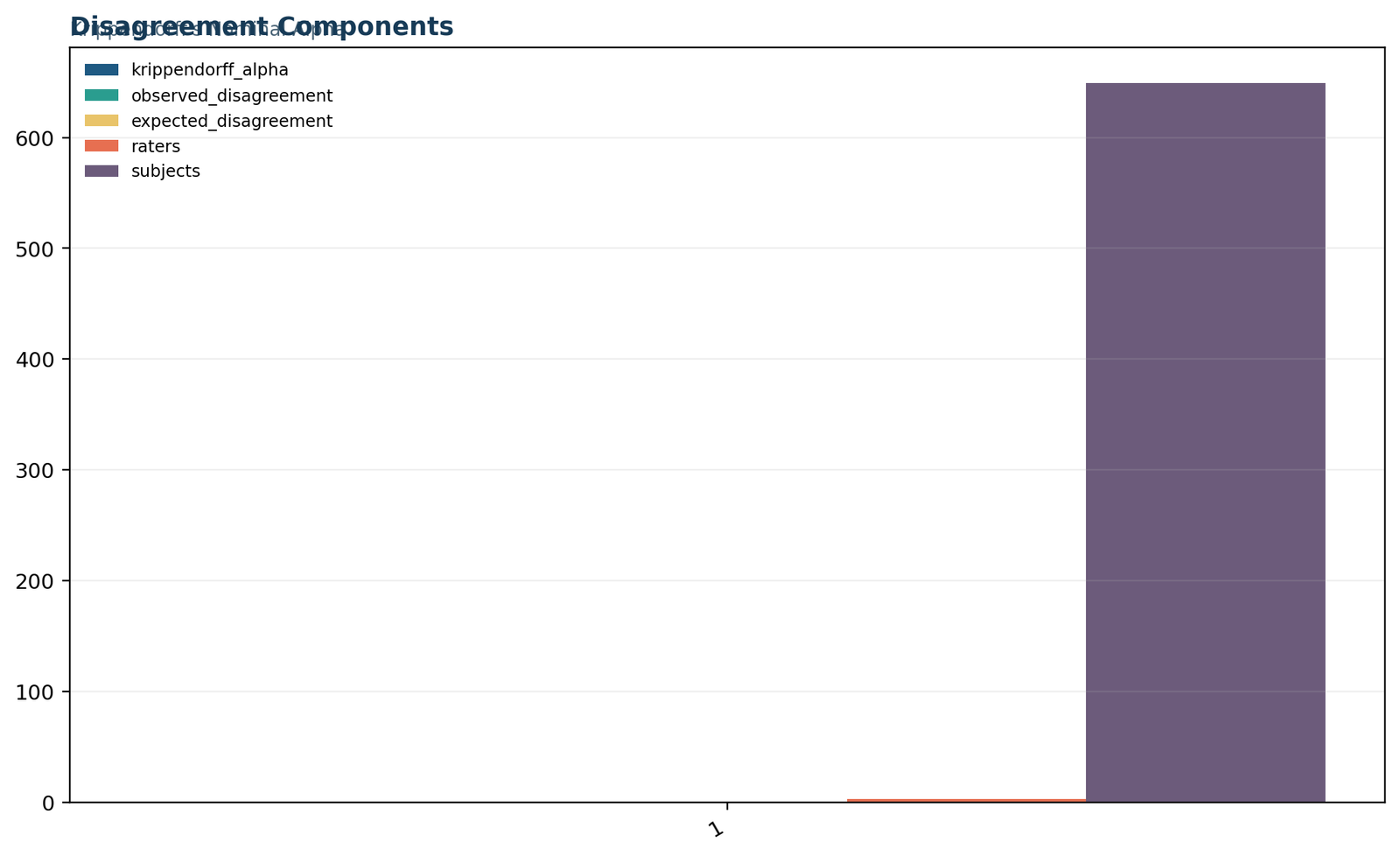
Python disagreement components
This chart places the coefficient beside observed disagreement, expected disagreement, source count and subject count. The mathematical relationship is alpha = 1 − Dₒ/Dₑ; it is not a sum or difference of the plotted bar heights.
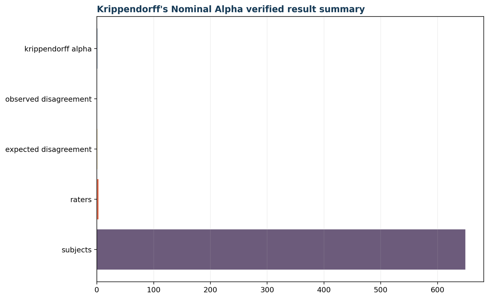
Python verified result summary
The final summary repeats the exact result ledger and confirms that the Python output matches the R and Excel calculations. It is designed as a verification panel rather than a common-scale effect-size graph.
The Python analysis should retain full precision in saved tables and round only in the narrative. The exact values are 0.6423094697924543 for alpha, 0.21571648690292758 for observed disagreement and 0.603081347380823 for expected disagreement. Package version, Python version and missing-value representation should be stored in the transcript.
Broader preprocessing and categorical-table guidance is available in Categorical Data Analysis in Python and Reliability Analysis in Python. Those workflows should be used to confirm category counts before the agreement coefficient is interpreted.
Krippendorff’s Alpha in R: nominal method and matched charts
The R section follows the same full-width-first and paired-chart layout used by the supplied ideal post.
The Krippendorff’s Alpha R workflow must state the package, function, matrix orientation and measurement-level argument. The supplied R report independently confirms the same nominal coefficient and disagreement components as Python and Excel.
df <- read.csv("dataset.csv")

cut_grade <- function(x) {

cut(x, breaks = c(-Inf, 9, 13, Inf), labels = c(0, 1, 2))

}

ratings <- data.frame(

G1 = cut_grade(df$G1),

G2 = cut_grade(df$G2),

G3 = cut_grade(df$G3)

)# Convert to the orientation required by the selected function.

# Specify the nominal method and verify Do, De, and alpha independently.
Some R agreement functions expect rating sources in rows, while others accept units in rows. The dimensions must therefore be checked before interpretation. The output should explicitly identify three rating occasions and 649 subjects. A default interval method applied to numeric codes 0, 1 and 2 would answer a different question from nominal alpha.
R result summary
The full-width R placement confirms alpha = 0.642309, Dₒ = 0.215716, Dₑ = 0.603081, three sources and 649 subjects. It uses the same verified metrics as Python so the two implementations can be checked directly.
R pooled category counts
The R evidence reproduces 402 low, 1,047 middle and 498 high values. These margins sum to 1,947 and match the Calculations and Reporting sheets in the worked Excel workbook.
R rating-pattern frequencies
The R pattern placement confirms 439 unanimous students and 210 non-unanimous students. Every non-unanimous row contains a two-versus-one configuration and contributes two discordant pairs.
R disagreement components
Observed disagreement is only about 35.77% of expected disagreement. Subtracting this ratio from one gives Krippendorff’s Alpha = 0.642309.
R verified result summary
The R verification panel repeats the exact coefficient, disagreement values, number of sources and number of units. The values agree with the independently executed Python workflow.
The R report should include session information so the calculation can be reproduced after package updates. It should also identify the nominal distance and any missing-value rule. In this dataset all 649 rows are complete, so missingness does not affect the coefficient.
Additional preparation and interpretation support is available in Categorical Data Analysis in R and Reliability Analysis in R. The essential cross-check is that R reproduces the same category frequencies, Do, De and alpha as the other artifacts.
Krippendorff’s Alpha SPSS workflow and corrected interpretation
SPSS verifies the recoding and pairwise diagnostics, while the general alpha is independently cross-checked.
The supplied Krippendorff’s Alpha SPSS output verifies recoding, category frequencies, the subject-disagreement distribution and pairwise Cohen coefficients. The visible CROSSTABS commands do not directly calculate the general three-source alpha, so the final coefficient appears as a separately checked result ledger.
What the SPSS output verifies
SPSS imports 649 rows, recodes G1, G2 and G3 into three categories and computes D12, D13 and D23 mismatch indicators. The mean subject disagreement is 0.2157 with a standard deviation of 0.31213. Exactly 439 students have subject disagreement 0 and 210 have subject disagreement 0.67.
The frequency tables reproduce 157/340/152 for G1, 145/352/152 for G2 and 100/355/194 for G3. No values are missing.
What must be reported carefully
The G1–G2 crosstab gives Cohen’s Kappa = .634 and the G1–G3 crosstab gives Cohen’s Kappa = .591. These are pair-specific coefficients. They do not equal the pooled three-source Krippendorff’s Alpha.
The final SPSS echo reports expected disagreement = 0.6030813474, observed disagreement = 0.2157164869 and alpha = 0.6423094698, with cross-check status marked as pass.
COMPUTE d12=(G1_cat3<>G2_cat3).

COMPUTE d13=(G1_cat3<>G3_cat3).

COMPUTE d23=(G2_cat3<>G3_cat3).

COMPUTE subject_disagreement=(d12+d13+d23)/3.FREQUENCIES VARIABLES=G1_cat3 G2_cat3 G3_cat3 subject_disagreement.

CROSSTABS /TABLES=G1_cat3 BY G2_cat3 /STATISTICS=KAPPA.

CROSSTABS /TABLES=G1_cat3 BY G3_cat3 /STATISTICS=KAPPA.
SPSS displays significance values of .000 for the pairwise kappas. Standard reporting writes these as p < .001, never p = .000. The pairwise significance tests do not supply an alpha-specific p-value or confidence interval.
For data preparation, labels and pivot-table interpretation, see Categorical Data Analysis in SPSS and Reliability Analysis in SPSS.
Krippendorff’s Alpha Excel calculation and workbook audit
The spreadsheet exposes the complete path from raw grades to the verified nominal coefficient.
The worked Krippendorff’s Alpha Excel file is formula driven and includes Guide, Data_Input, Working, Calculations, Diagnostics and Reporting sheets. It exposes the row-level disagreement components and compares workbook results with independently verified Python and R references.
Workbook structure
| Sheet | Purpose | Key check |
|---|---|---|
| Guide | Documents the design, variables, null hypothesis and formula | Nominal coincidence disagreement |
| Data_Input | Stores unchanged G1, G2 and G3 values | 649 source rows |
| Working | Creates categories and D12, D13 and D23 mismatch indicators | Row-level subject disagreement |
| Calculations | Reproduces Dₒ and stores exact verified metrics | Alpha = 0.6423094698 |
| Diagnostics | Documents assumptions, scope and row counts | 649 expected and 649 analyzed |
| Reporting | Compares workbook and verified values | Absolute differences effectively zero |
Core formula logic
| Excel component | Formula logic | Worked value |
|---|---|---|
| Category recoding | Use identical IF or lookup thresholds for G1, G2 and G3. | Low / middle / high |
| D12 | =--(G1_Class<>G2_Class) | 0 or 1 |
| D13 | =--(G1_Class<>G3_Class) | 0 or 1 |
| D23 | =--(G2_Class<>G3_Class) | 0 or 1 |
| Subject disagreement | =AVERAGE(D12,D13,D23) | 0 or 0.666667 |
| Observed disagreement | Average subject disagreement over 649 rows. | 0.2157164869 |
| Final alpha | =1-Observed_Disagreement/Expected_Disagreement | 0.6423094698 |
The Reporting sheet shows zero absolute difference for alpha, expected disagreement, rater count and subject count. The observed-disagreement difference is approximately 2.78 × 10⁻¹⁶, which is only floating-point representation and has no substantive effect.
Missing data, number of raters and Krippendorff’s Alpha levels
The generality of the method comes from pairable values and an explicit disagreement distance.
A major advantage of Krippendorff’s Alpha is that units do not need the same number of valid ratings. The method uses all pairable values and allows the disagreement function to reflect nominal, ordinal, interval, ratio or specialized measurement structures.
Missing ratings
A unit contributes whenever at least two usable values remain. If one of three ratings is missing, the remaining two can still form a pair. A unit with zero or one valid value cannot contribute to within-unit disagreement.
This computational flexibility does not make informative missingness harmless. If difficult units are skipped more often, the retained ratings may overstate reliability. Reports should state how many values each unit supplied and whether any missing code was treated as a legitimate category.
Variable numbers of raters
Different units may be rated by different subsets of coders. The coincidence framework pools the available within-unit pairs and preserves the intended distance rule. This makes the coefficient useful in annotation projects and observational studies where complete rating matrices are difficult to obtain.
A single pooled alpha still cannot identify which source is inconsistent. Pairwise tables and leave-one-source-out sensitivity analyses remain useful diagnostics.
| Krippendorff’s Alpha form | Suitable data | Disagreement definition | Example |
|---|---|---|---|
| Nominal | Unordered categories | 0 for equality; 1 for inequality | Topic labels, diagnosis classes, exact grade bands |
| Ordinal | Ordered categories | Greater category separation receives greater penalty | Likert responses, severity classes, ordered grade bands |
| Interval | Equal-interval measurements | Squared numerical difference | Standardized ratings or interval-scale scores |
| Ratio | Positive values with meaningful zero | Relative difference appropriate to ratio data | Duration, concentration or positive measurements |
| Custom | Specialized value systems | Research-defined distance or cost | Circular directions or domain-specific error costs |
The primary analysis is nominal because it asks whether the exact low, middle or high band is reproduced. The categories are ordered, so an ordinal sensitivity analysis is reasonable. Because every observed mismatch is adjacent and no low-high disagreement occurs, ordinal alpha would likely be higher. It would not replace the nominal result; it would answer a different question.
Krippendorff’s Alpha vs Cohen’s Kappa, Fleiss Kappa and ICC
Choose the coefficient that matches the number of sources, scale and missing-data structure.
The Krippendorff’s Alpha vs Cohen’s Kappa and Fleiss Kappa vs Krippendorff’s Alpha questions are common because all three are chance-corrected agreement coefficients. They differ in design, data representation, missing-data handling and scale flexibility.
| Method | Typical design | Primary question | Main advantage | Main caution |
|---|---|---|---|---|
| Krippendorff’s Alpha | Two or more sources; incomplete matrices possible | How much expected disagreement is removed? | Multiple scale levels and flexible missingness | Requires a defensible distance and design interpretation |
| Cohen’s Kappa | Two paired categorical sources | How much pairwise agreement exceeds chance? | Familiar two-rater contingency-table interpretation | Not a general multi-rater coefficient |
| Fleiss Kappa | Multiple nominal ratings | How much multi-rater nominal agreement exceeds chance? | Useful for fixed nominal category counts | Different chance formulation and less scale flexibility |
| Weighted Kappa | Two ordered categorical sources | How much weighted pairwise agreement exceeds chance? | Penalizes distant disagreements more heavily | Weights must be justified and only two sources are compared |
| Intraclass Correlation Coefficient | Quantitative ratings under a variance model | How reliable are numerical measurements? | Preserves magnitude information | Model choice changes the estimand |
| Cronbach’s Alpha | Multiple scale items | How internally consistent are the items? | Widely used for scale development | Not a direct rater-agreement coefficient |
| Spearman correlation | Two ordered variables | How strongly are ranks monotonically associated? | Measures ordinal association | High association can coexist with poor agreement |
A chi-square association test or correlation coefficient can show that sources are related without demonstrating exact identity. Agreement methods privilege the diagonal or small disagreement distances. The selection should be based on the question, not on which method yields the largest coefficient.
Diagnostics, sensitivity checks and common Krippendorff’s Alpha mistakes
A defensible reliability analysis combines the coefficient with design, prevalence and disagreement-pattern checks.
A credible Krippendorff’s Alpha interpretation combines the coefficient with category prevalence, pairwise tables, pattern frequencies, scale-level sensitivity and uncertainty. The numerical calculation can be correct while the substantive claim remains weak if the units, categories or reliability standard are poorly defined.
Before calculation
After calculation
Common mistakes
| Mistake | Why it is wrong | Better practice |
|---|---|---|
| Calling alpha a correlation | Agreement and association are different estimands | Explain Dₒ, Dₑ and exact identity |
| Reporting 0.642 as 64.2% of subjects agreeing | Alpha is a proportional reduction in disagreement | Report raw agreement separately |
| Treating p > .05 pairwise kappa output as the alpha test | Pairwise kappa inference is not pooled alpha inference | Use an alpha-specific interval or bootstrap |
| Ignoring category prevalence | Expected disagreement depends on pooled margins | Report pooled counts and rare categories |
| Using numeric codes as interval values by default | Codes may be labels rather than equal-interval measurements | Specify nominal or ordinal distance explicitly |
| Claiming reliability because alpha is above zero | Above-chance agreement may still be unusable | Compare with a prespecified minimum |
| Ignoring temporal change in G1, G2 and G3 | Mismatch may represent real development | Describe the design as category stability |
A confidence interval is not included in the supplied reports. For uncertainty estimation, bootstrap whole students with replacement and retain all ratings within each resampled student. Resampling individual cells would destroy the within-unit structure. The lower confidence bound should be compared with the required reliability minimum, not merely with zero.
Threshold sensitivity is also important. Grades of 9 and 10 are only one point apart but fall into different categories, while grades of 10 and 13 remain in the same category. Recalculate alpha under defensible alternative boundaries to determine whether the conclusion is stable or created by one arbitrary cut point.
Extended interpretation checks
Reliability versus validity
Krippendorff’s Alpha addresses reproducibility of recorded values, not whether the categories represent the intended construct. A perfectly reproducible classification can still be invalid if the thresholds do not reflect educational meaning. Conversely, a theoretically valid category system can be recorded unreliably. The reliability result should therefore be discussed as one requirement for defensible measurement rather than a complete validation study.
Category-prevalence sensitivity
Expected disagreement preserves the pooled category frequencies. Two studies can have the same raw agreement and different alpha values when their prevalence structures differ. Cross-study comparisons should include category margins, number of raters and missing-data patterns instead of ranking projects by one coefficient.
Decision consequences
A minimum acceptable coefficient should be connected to the harm caused by disagreement. Exploratory descriptive coding may tolerate more uncertainty than clinical diagnosis, legal classification or high-stakes placement. The common .667 and .800 conventions are useful reference points, but the substantive cost of error should determine the final standard.
Threshold sensitivity
The grade-band boundaries control which one-point differences become full nominal disagreements. A grade of 9 and a grade of 10 are treated as different categories, while grades of 10 and 13 agree. Repeating the analysis with defensible alternative boundaries shows whether the conclusion is stable or dependent on one cut point.
Ordinal sensitivity
Because low, middle and high are ordered and every observed mismatch is adjacent, ordinal alpha may be larger than nominal alpha. That result would show closeness on an ordered scale, not exact category identity. Both coefficients can be reported when the distinction is meaningful and planned in advance.
Source-specific diagnosis
The pooled coefficient does not identify which source contributes most to disagreement. Pairwise tables show that G1–G3 has the weakest kappa and the largest directional shift, while G2–G3 has the strongest pairwise agreement. Leave-one-source-out analysis can provide another diagnostic without replacing the primary coefficient.
Bootstrap uncertainty
A bootstrap confidence interval should resample whole students and retain all three ratings within each selected row. Cell-level resampling would destroy the dependence structure that defines agreement. The interval should be compared with the required reliability minimum rather than used only to test whether alpha exceeds zero.
Generalization
Reliability is a property of a measurement process applied to a population of units. The 649 students provide substantial information, but the conclusion may not generalize to other schools, subjects, grading systems or performance ranges. Sampling scope belongs in the limitations section.
How to report Krippendorff’s Alpha in APA style
Include the design, category rules, disagreement components and a restrained reliability conclusion.
An APA-style Krippendorff’s Alpha report should identify the units, sources, number of ratings, category definitions, measurement level, disagreement function, coefficient, observed disagreement, expected disagreement, missing-data rule and practical conclusion.
APA-style result
Compact technical report
Krippendorff’s Alpha: α = 0.642309; Do = 0.215716; De = 0.603081; three nominal rating occasions; 649 units; 1,947 pooled values; complete three-way agreement = 67.64%.
Reporting checklist
Do not report that 64.23% of students agreed. Do not report an alpha-specific p-value from the pairwise SPSS kappa tables. Do not describe the sources as independent coders. The strongest interpretation states that grade-band classifications show meaningful but insufficient stability across the three occasions.
The discussion can add that disagreements are adjacent and predominantly upward over time. G1–G3 has the weakest pairwise kappa and the largest directional shift, while G2–G3 has the strongest pairwise kappa. These patterns explain the coefficient and prevent a black-box reliability conclusion.
Krippendorff’s Alpha PDF, Excel and software downloads
Open the exact Python, R, SPSS and Excel artifacts used in the worked analysis.
The downloadable Krippendorff’s Alpha PDF reports and worked Excel workbook allow readers to verify the coefficient across four analysis environments. Every download refers to the same 649-subject nominal analysis and the same exact result ledger.
R reportIndependent R calculation with the same dimensions, nominal distance and verified values.Open R PDF →
SPSS outputCategory frequencies, subject disagreement, pairwise kappas and the checked alpha result ledger.Open SPSS PDF →
Worked Excel fileRaw data, formula-driven recoding, disagreement components, diagnostics and reporting checks.Download Excel →
Krippendorff’s Alpha methodological references and software documentation
Primary methodological sources and implementation documentation used to verify the analysis.
The terminology, formula and interpretation of Krippendorff’s Alpha should be checked against methodological and software documentation rather than copied from short summaries. The source cards below identify the primary reference types used for verification without adding outbound links to the public article.
Krippendorff methodology
Klaus Krippendorff’s methodological work defines alpha through observed and expected disagreement, coincidence matrices, missing-data flexibility and scale-appropriate distance functions.
Reliability research
Methodological articles by Krippendorff and collaborators explain why one standard coefficient should accommodate multiple raters, incomplete data and different levels of measurement.
Software documentation
The Python and R implementations should be checked against the official documentation for the selected package and function, including matrix orientation, nominal method, missing-value codes and version-specific behavior.
Krippendorff’s Alpha FAQs
Answers to the interpretation, calculation and software questions most often missed in brief summaries.
These Krippendorff’s Alpha FAQs answer the highest-value search questions: what the coefficient measures, how it is calculated, acceptable values, negative results, missing ratings, software workflows and comparisons with Cohen’s Kappa and Fleiss Kappa.
What is Krippendorff’s Alpha?
What does Krippendorff’s Alpha measure?
What is a good Krippendorff’s Alpha?
How do you calculate Krippendorff’s Alpha?
Can Krippendorff’s Alpha be negative?
Can Krippendorff’s Alpha handle missing data?
How many raters are required?
What is the difference between Krippendorff’s Alpha and Cohen’s Kappa?
What is the difference between Fleiss Kappa and Krippendorff’s Alpha?
Should low, middle and high use nominal or ordinal alpha?
How do I calculate Krippendorff’s Alpha in SPSS?
How should Krippendorff’s Alpha = .642 be interpreted?
Related statistical guides
Continue with the reliability, categorical agreement and software guides most closely connected to Krippendorff’s Alpha.