
Corrected Item-Total Correlation: Formula, Interpretation, Cutoff, SPSS, Python, R and Excel Guide
Corrected Item-Total Correlation measures how strongly one item relates to the total score formed from all of the other items. This complete guide explains the definition, formula, acceptable cutoff, negative values, Cronbach’s alpha relationship, item deletion decisions, assumptions, calculator logic, Python, R, SPSS and Excel workflows, APA reporting, ten chart interpretations and four downloadable analysis files through a six-item worked example with 649 complete records.
The six items do not function as a strong single internally consistent scale
The worked Corrected Item-Total Correlation analysis correlates each target item with the sum of the other five items. The highest coefficient is 0.226597 for famrel, while the lowest is -0.104770 for goout. The mean across all six corrected coefficients is only 0.061453. None reaches the frequently used 0.30 screening benchmark, and three coefficients are negative. These findings indicate weak item-rest alignment for the proposed six-item composite.
The SPSS reliability output supports the same conclusion. Raw Cronbach’s alpha is 0.112 and standardized alpha is 0.169 for 649 complete cases. Deleting goout produces the largest alpha-if-deleted value, approximately 0.234, but that value remains low. The result does not justify deleting items mechanically. It indicates that the six variables may represent several different concepts rather than one coherent construct and that the scale definition, item direction and measurement model require substantive review.
Core values
Contents
What Is Corrected Item-Total Correlation?
The statistic removes an item from its own comparison total so the association is not inflated by self-inclusion.
Corrected Item-Total Correlation is the Pearson correlation between an item and the sum, mean or score formed from the remaining items in the same proposed scale. It is also called an item-rest correlation, corrected item-total coefficient or item-remainder correlation. The word corrected is essential. An ordinary item-total correlation places the target item inside the total and then correlates the item with a score that partly contains itself. That built-in overlap tends to raise the coefficient even when the item has little genuine relationship with the other items. The corrected version removes the target item first and therefore provides a cleaner test of whether the item behaves like the rest of the scale.
The central research question is not simply whether an item has variance or whether its mean looks reasonable. The question is whether people who obtain a relatively high score on one item also tend to obtain a relatively high score on the remaining scale content. A positive and reasonably large Corrected Item-Total Correlation suggests that the item participates in the same broad ordering of respondents as the other items. A coefficient close to zero suggests weak linear alignment. A negative coefficient suggests that high values on the item tend to accompany low values on the rest score, which may reflect reversed wording, incorrect coding, a multidimensional construct or an item that does not belong in the proposed scale.
The statistic is most useful during scale development, questionnaire evaluation, test-item review, reliability analysis and quality control of composite scores. It complements rather than replaces content validity, factor analysis, response-process evidence and substantive judgment. A scale can have acceptable coefficients while still measuring the wrong construct, and a theoretically important item can have a modest coefficient because it covers a unique but necessary part of the domain. The descriptive statistics guide helps establish the means, standard deviations and score ranges that should be checked before interpreting item-rest relationships.
In the present worked example, Corrected Item-Total Correlation is calculated for six variables: family relationship quality, free time, going out, reverse-scored weekday alcohol use, reverse-scored weekend alcohol use and health status. Each item is correlated with the sum of the other five. The results are intentionally diagnostic: the mean coefficient is 0.061453, which is far below a common 0.30 screening rule. This pattern indicates that the six variables should not be treated as a strong single scale without additional theory, recoding review and structural analysis.
When to Use Corrected Item-Total Correlation
Use it for multi-item instruments when each row represents one respondent and the items are intended to contribute to a shared score.
Use Corrected Item-Total Correlation when several items are intended to represent a common construct and you need an item-level diagnostic before computing or reporting a composite score. Typical applications include Likert questionnaires, psychological tests, educational scales, customer-experience indices, clinical symptom inventories and workplace surveys. The method is appropriate when the item responses can be treated as quantitative enough for a Pearson item-rest association or when a clearly justified ordinal alternative is used. Every coefficient must be calculated on comparable cases and with the target item excluded from its rest score.
The analysis is especially valuable after reverse-scored items have been recoded. A negative wording direction can be legitimate, but the numerical direction must be aligned before the reliability calculation. In the worked data, weekday and weekend alcohol-use variables are transformed as Dalc_R = 6 - Dalc and Walc_R = 6 - Walc. Higher transformed scores therefore represent lower reported alcohol use. Without that transformation, the direction of their relationships with positively framed items would be harder to interpret. The calculation still shows that reverse scoring alone does not create a coherent scale: one transformed alcohol item has a small positive coefficient and the other remains slightly negative.
Do not use Corrected Item-Total Correlation as a general measure of agreement between raters. For two categorical raters, use Cohen's Kappa guide; for more than two categorical raters, use Fleiss Kappa guide; and for continuous ratings, consider the intraclass correlation coefficient guide. Do not use the item-rest coefficient as proof of test-retest stability, interrater reliability or criterion validity. Those are different measurement questions requiring different designs. The item-rest statistic is specifically about an item’s relationship with the remainder of a proposed multi-item score.
The method is also not a substitute for factor analysis. A set of items can show moderate item-rest coefficients because several related dimensions share a general factor, while a factor model may reveal meaningful subscales. Conversely, a small set can have unstable correlations even when the theory is sound. Use Corrected Item-Total Correlation as one line of evidence in a broader instrument-development workflow: inspect wording and coding, review missingness, examine distributions, calculate the correlation matrix, evaluate alpha or omega, study dimensionality and then decide whether the total score is defensible.
Variables and Coding for the Corrected Item-Total Correlation Example
The item direction, numerical range and substantive meaning must be documented before any reliability statistic is interpreted.
The worked Corrected Item-Total Correlation example uses 649 complete student records and six bounded variables. The first three variables are famrel, freetime and goout. The last three are reverse-scored weekday alcohol use, reverse-scored weekend alcohol use and self-reported health. All six variables have values from 1 to 5 after transformation. Having a common numeric range simplifies presentation, but equal ranges do not prove that the items measure one construct.
| Item | Public meaning | Coding used | Mean | SD |
|---|---|---|---|---|
| famrel | Quality of family relationships | 1 to 5; higher = better | 3.9307 | 0.9557 |
| freetime | Free time after school | 1 to 5; higher = more | 3.1803 | 1.0511 |
| goout | Frequency of going out with friends | 1 to 5; higher = more | 3.1849 | 1.1758 |
| Dalc_R | Reverse-scored weekday alcohol use | 6 − Dalc; higher = lower use | 4.4977 | 0.9248 |
| Walc_R | Reverse-scored weekend alcohol use | 6 − Walc; higher = lower use | 3.7196 | 1.2844 |
| health | Current health status | 1 to 5; higher = better | 3.5362 | 1.4463 |
The item means show that Dalc_R is concentrated toward the high end because many students report low weekday alcohol use. Health has the largest standard deviation, while Dalc_R has the smallest. Distribution differences matter because a restricted item can have a lower correlation even when its content is relevant. The standard deviation guide explains how standard deviation reflects score spread and why low variability can limit the size of a Pearson relationship.
The six variables do not obviously define a single narrow latent trait. Family relationships, leisure time, social activity, alcohol-use behavior and health status are conceptually distinct. The worked result therefore demonstrates an important principle: Corrected Item-Total Correlation should evaluate a scale that was defined by theory, not manufacture a construct from convenient variables. A low coefficient may correctly warn that the proposed total combines heterogeneous content.
All 649 records are complete for the six items, so the SPSS reliability procedure uses listwise N = 649 with no excluded cases. In other datasets, the analyst must report whether the coefficients use listwise deletion, pairwise deletion, imputation or a model-based missing-data method. Different missing-data rules can produce different rest scores and different coefficients. The coding table, sample size and missing-data decision should therefore appear in the analysis record and the final report.
Corrected Item-Total Correlation Formula and Statistical Meaning
The target item is correlated with a rest score formed without that item.
Let Xi denote the target item for person i, and let T denote the full scale total. The corrected rest score is T − X. The Corrected Item-Total Correlation for item j is the Pearson correlation between Xj and the total of all items except Xj. If the scale uses an average rather than a sum, the coefficient is unchanged when every person has the same number of observed items because multiplying the rest score by a positive constant does not change a correlation.
The target item is excluded from the comparison total. This is the defining correction.
The Pearson form can be written as the covariance between the target item and the rest score divided by the product of their standard deviations. This expression clarifies three reasons a Corrected Item-Total Correlation can be small: the item and rest score may not covary, the relationship may be nonlinear, or one variable may have restricted variation. The coefficient is bounded between -1 and +1. Positive values indicate that higher item scores tend to accompany higher rest scores. Negative values indicate an inverse ordering. Values near zero indicate little linear association.
Here, x is the target item and y is the score made from the remaining items.
The null hypothesis for an inferential Pearson test is that the population item-rest correlation equals zero. However, statistical significance is not the main item-retention criterion. With 649 records, a small coefficient can be statistically detectable but still too weak to support a useful scale. For example, Dalc_R has a coefficient of 0.139144 with a very small p-value, yet the magnitude remains weak. The p-value and significance guide explains why effect magnitude and p-value answer different questions.
Some software labels the output ‘Corrected Item-Total Correlation’ even though the comparison is technically item versus remainder. That label is conventional and should be retained when explaining SPSS tables. The analyst should nevertheless understand the computation, because a manually calculated ordinary item-total correlation will not match the corrected SPSS column. Always confirm that the target item was removed before comparing results across software.
Complete Corrected Item-Total Correlation Results for All Six Items
The item-level pattern is more informative than a single mean coefficient.
The complete Corrected Item-Total Correlation results are shown below. The coefficients are calculated from the same 649 complete cases in Python and R and cross-checked against the SPSS Item-Total Statistics table. The final column shows Cronbach’s alpha if the named item is deleted. These columns answer related but distinct questions: the item-rest coefficient describes how the item aligns with the remainder, while alpha if deleted describes how the overall internal-consistency coefficient changes after removal.
| Item | Mean | SD | Corrected r | Two-tailed p | Alpha if deleted |
|---|---|---|---|---|---|
| famrel | 3.9307 | 0.9557 | 0.226597 | < .001 | -0.056486 |
| freetime | 3.1803 | 1.0511 | 0.151318 | < .001 | -0.002364 |
| goout | 3.1849 | 1.1758 | -0.104770 | .0076 | 0.234087 |
| Dalc_R | 4.4977 | 0.9248 | 0.139144 | < .001 | 0.021909 |
| Walc_R | 3.7196 | 1.2844 | -0.033120 | .3996 | 0.177823 |
| health | 3.5362 | 1.4463 | -0.010454 | .7904 | 0.165338 |
famrel has the strongest Corrected Item-Total Correlation at 0.226597. That is positive and statistically detectable, but it remains below a common 0.30 screening threshold. freetime and Dalc_R are also positive at 0.151318 and 0.139144. The positive direction means that respondents with higher values on those items tend to have slightly higher sums on the other five items. The relationships are nevertheless weak.
goout has the most concerning coefficient, -0.104770. This is not a trivial rounding artifact: the inverse association is statistically detectable at p = .0076. Walc_R and health are also negative, but their magnitudes are close to zero and their Pearson tests are not statistically significant. A negative Corrected Item-Total Correlation is a diagnostic flag, not an automatic deletion command. The item wording, coding, content and factor structure should be examined first.
The mean corrected coefficient is 0.061453. A mean can summarize the general weakness, but it hides the mixture of positive and negative items. The full pattern suggests that the proposed total score combines dimensions that do not move together consistently. Removing goout raises alpha from 0.111763 to 0.234087, which is the largest improvement, but the resulting coefficient is still too low for a dependable one-dimensional score in most applications. The substantive conclusion is scale revision, not cosmetic item deletion.
What Is an Acceptable Corrected Item-Total Correlation?
Cutoffs are screening conventions, not universal laws. Interpret magnitude with purpose, sample, item content and measurement model.
A frequently used practical rule treats a Corrected Item-Total Correlation of 0.30 or higher as acceptable for an established item, values from about 0.20 to 0.29 as marginal, and values below 0.20 as weak. Some exploratory scale-development contexts temporarily retain items around 0.20 when the content is essential or the scale is short. More demanding applications may prefer 0.40 or higher. These ranges are conventions rather than mathematical boundaries, and they should not be presented as universal proof of validity.
| Corrected r range | Common screening interpretation | Recommended action |
|---|---|---|
| Negative | Opposite direction from the rest score | Check coding, wording, construct and dimensionality immediately |
| 0.00 to 0.19 | Weak item-rest alignment | Review content, variance, response pattern and scale definition |
| 0.20 to 0.29 | Marginal or exploratory | Retain only with theoretical and structural justification |
| 0.30 to 0.49 | Often acceptable | Review alongside alpha, omega, factor loadings and content coverage |
| 0.50 and above | Strong alignment | Check for redundancy as well as consistency |
The phrase ‘acceptable corrected item total correlation’ should therefore be answered conditionally. A value is acceptable when it supports the intended use of the score, remains stable across relevant samples, aligns with the factor structure and preserves necessary content. A 0.28 coefficient may be defensible for a unique item in a broad early-stage construct, while a 0.35 coefficient may still be problematic if the item loads on the wrong factor or introduces differential item functioning.
Very high values are not automatically ideal. If many items have coefficients above 0.80, the scale may contain repeated or nearly synonymous wording. Redundancy can inflate internal consistency without improving construct coverage. The goal is coherent breadth: items should share enough variance to support a total score while still sampling distinct aspects of the intended domain.
In the worked analysis, every Corrected Item-Total Correlation is below 0.30. The maximum of 0.226597 is marginal at best, three items are negative and the mean is 0.061453. The cutoff conclusion is therefore clear: the six-item combination does not meet a conventional item-rest screening standard. This conclusion remains a measurement judgment rather than a significance test. The confidence interval guide can be used when precision around a coefficient is important, but a narrow interval around a weak value does not make the item strong.
How to Interpret a Negative Corrected Item-Total Correlation
A negative coefficient means that the item orders respondents in the opposite direction from the remaining score.
A negative Corrected Item-Total Correlation is one of the most useful warnings in an item analysis. It means that respondents with high scores on the target item tend to have low scores on the rest score, or vice versa. The first check is direction. If the item is negatively worded, confirm that it was reverse scored correctly. For a 1-to-5 response scale, the common transformation is 6 - original score. A coding error can turn an otherwise positive item-rest relationship negative.
The second check is content. An item can be correctly coded and still be inversely related because it measures a different behavior or dimension. In this example, goout has a coefficient of -0.104770 even after the alcohol-use items have been directionally aligned. Going out with friends may reflect social activity rather than the same dimension as family relationship quality, lower alcohol use and self-rated health. The negative result may therefore be substantively meaningful rather than erroneous.
The third check is response quality. A confusing item, double-barreled question, ambiguous time frame, translation problem or unusual response option can weaken or reverse the association. Examine item frequencies, missingness, floor and ceiling concentration, and subgroup patterns. The guide to frequency and relative frequency tables is useful for checking whether one category dominates or whether the response distribution differs sharply from the other items.
The fourth check is dimensionality. If a scale contains two factors with opposite scoring directions, items from one factor can have negative correlations with the total of the other factor. A factor analysis or clearly planned subscale analysis may show that the item belongs elsewhere. Do not delete a negative item merely to raise alpha until the theoretical structure has been reviewed.
In the worked results, deleting goout raises alpha to approximately 0.234. That improvement confirms that the item contributes negative covariance to the proposed total. Yet the resulting alpha remains low, so goout is not the only problem. The correct conclusion is that the overall item set requires redesign. A negative Corrected Item-Total Correlation should trigger a diagnostic sequence—coding, content, distribution, subgroup behavior and dimensionality—not an automatic deletion rule.
Corrected Item-Total Correlation and Cronbach’s Alpha
Item-rest coefficients explain local item behavior; alpha summarizes covariance across the complete item set.
Corrected Item-Total Correlation and Cronbach’s alpha are connected because both depend on relationships among items, but they are not interchangeable. The item-rest coefficient is calculated separately for each item. Cronbach’s alpha combines the number of items, their variances and the variance of the total score into one internal-consistency estimate. An instrument can have one weak item-rest coefficient while maintaining a reasonably high alpha, especially when it contains many strong items. Conversely, a short heterogeneous scale can have low alpha even when one or two items have modest positive coefficients.
k is the number of items, the numerator sum contains item variances, and sT² is the variance of the total score.
For the six-item worked scale, raw alpha is 0.111763 and standardized alpha is 0.168910. The standardized coefficient can also be obtained from the average inter-item correlation, which is approximately 0.032763. Both alpha values are very low. Standardization raises the coefficient slightly because it removes differences in item variance, but it cannot repair inconsistent covariance direction.
Alpha if item deleted helps identify which item is reducing the coefficient. Deleting goout produces the largest value, 0.234087. Deleting Walc_R produces 0.177823, and deleting health produces 0.165338. Deleting famrel or freetime results in a slightly negative alpha because the average covariance among the remaining items becomes negative. SPSS explicitly warns that a negative alpha-if-deleted value reflects negative average covariance and that item coding should be checked.
Do not select items solely by maximizing alpha. Alpha can increase when a unique, content-valid item is removed, and it can become very high when redundant items are added. Review Corrected Item-Total Correlation, alpha if deleted, inter-item correlations, item means, factor structure and content coverage together. For dichotomous 0/1 items, the related KR-20 calculator applies the KR-20 form, which is algebraically linked to alpha under consistent variance conventions.
The worked scale illustrates a crucial distinction: removing the worst item improves a numerical coefficient but does not create a strong measure. An alpha of 0.234 after deletion remains far below common expectations. The priority should be to define the construct, develop or select items that represent it coherently, pilot the revised instrument and then repeat the Corrected Item-Total Correlation analysis.
Inter-Item Correlations, Corrected Item-Total Correlation and Dimensionality
The correlation matrix reveals which item pairs create the positive and negative item-rest pattern.
The inter-item matrix explains why the Corrected Item-Total Correlation values are weak. Some item pairs are positively related, while others are clearly negative. The strongest positive pair is Dalc_R with Walc_R, r = 0.617, which is expected because both are reverse-scored alcohol-use frequency measures. The strongest negative pair is goout with Walc_R, r = -0.389. These opposing clusters reduce the coherence of the overall six-item total.
| Item | famrel | freetime | goout | Dalc_R | Walc_R | health |
|---|---|---|---|---|---|---|
| famrel | 1.000 | .129 | .090 | .076 | .094 | .110 |
| freetime | .129 | 1.000 | .346 | -.110 | -.120 | .085 |
| goout | .090 | .346 | 1.000 | -.245 | -.389 | -.016 |
| Dalc_R | .076 | -.110 | -.245 | 1.000 | .617 | -.059 |
| Walc_R | .094 | -.120 | -.389 | .617 | 1.000 | -.115 |
| health | .110 | .085 | -.016 | -.059 | -.115 | 1.000 |
freetime and goout correlate at 0.346, forming a leisure or social-activity cluster. The alcohol items form another cluster. Family relationship quality has only small positive correlations with the other items, ranging from 0.076 to 0.129. Health has small positive relationships with family relationship and free time but negative relationships with both alcohol variables after reverse scoring. The matrix therefore does not resemble a single compact block of uniformly positive associations.
Because each Corrected Item-Total Correlation combines five pairwise relationships into one item-rest association, the coefficient reflects this mixture. For example, goout is positively related to free time but negatively related to the reverse-scored alcohol variables. The negative relationships dominate its rest-score covariance, producing the lowest item-rest coefficient. Similarly, Walc_R has a strong positive relationship with Dalc_R but negative relationships with free time, going out and health, leaving its overall corrected coefficient near zero.
This pattern strongly suggests multidimensionality or an improperly defined composite. A factor analysis would be a logical next step if theory supports one or more latent dimensions. The analyst might find a social-activity factor, an alcohol-use factor and separate family or health indicators. A total score that collapses these domains would be difficult to interpret. The Corrected Item-Total Correlation analysis does not identify the final factor solution, but it clearly shows that a one-score assumption needs stronger evidence.
Corrected Item-Total Correlation Assumptions and Diagnostic Checks
The Pearson item-rest coefficient requires more than a complete spreadsheet and a software command.
The first assumption is correct scale construction. Every item must have a documented direction, and reverse-scored items must be transformed before the total is calculated. The rest score must exclude the target item. The same set of items should be used consistently across respondents, or the scoring rule for partial data must be explicitly defined. Violating these conditions changes the meaning of Corrected Item-Total Correlation.
The second assumption is an approximately linear relationship between the item and the rest score when Pearson correlation is used. Bounded ordinal items often produce stepped scatterplots rather than smooth continuous clouds, but the average rest score should still change in a roughly monotonic linear direction across response categories. Plot the mean rest score by each item category and inspect unusual reversals. The correlation assumptions guide provides a fuller checklist for Pearson linearity, influential observations and alternative rank-based coefficients.
The third assumption is adequate variation. An item with an extreme ceiling or floor can have a small coefficient because it does not distinguish respondents. Review the mean, standard deviation and category frequencies. In this example, Dalc_R has the highest mean and smallest standard deviation, indicating concentration toward lower weekday alcohol use. Its corrected coefficient is positive but weak. Restricted range is one possible contributor, although the heterogeneous construct remains the larger issue.
The fourth assumption is independent rows. The 649 records are treated as independent students. Clustered designs, repeated observations or duplicated cases can make conventional p-values and confidence intervals misleading. Item analysis for multilevel data may require cluster-aware estimation or separate examination across schools, sites or time points.
The fifth assumption is that missing data are handled transparently. SPSS uses listwise complete cases in the reliability procedure shown here. If missingness is substantial, complete-case coefficients may represent a selective sample. Compare item missingness, investigate patterns and use a justified scoring rule. The sixth assumption is that outliers and data errors have been checked. Although bounded 1-to-5 items limit extreme raw values, an impossible code such as 9 or 99 can distort means, totals and correlations. The outlier detection guide offers a general workflow for identifying unusual values.
Normality is not required for the descriptive meaning of a Pearson coefficient, but it matters for small-sample inferential tests and confidence intervals. With bounded ordinal items, distributional departures are common. Report the coefficient primarily as an item diagnostic, use plots and consider Spearman or polychoric methods when the measurement level and sample justify them. The Shapiro-Wilk test guide should not be used as a mechanical pass-or-fail gate for every Likert item.
How to Calculate Corrected Item-Total Correlation by Hand
A transparent row-wise rest score makes software results easy to audit.
Begin with a data matrix in which rows are respondents and columns are items. Confirm that all items point in the same intended direction. For the first target item, create a new column equal to the sum of all remaining items. Correlate the target item with that new rest-score column. Repeat the process for every item, rebuilding the rest score each time. This repeated exclusion is the manual essence of Corrected Item-Total Correlation.
For famrel, the comparison total is freetime + goout + Dalc_R + Walc_R + health. That rest score has a mean of 18.1186. Correlating it with famrel produces 0.226597. For goout, the rest score excludes goout and includes the other five items; the resulting coefficient is -0.104770. The rest score is different for each item, so one fixed total column cannot be reused unless the target item is subtracted from the full total.
A common shortcut is to calculate the full score once and then use rest = full total - item. This is algebraically equivalent to summing the remaining items when there are no scoring complications. It is also convenient in Excel, Python and R. When a scale uses item weights, however, subtract the weighted item contribution rather than the raw item. When a mean score is used with missing responses, ensure that the denominator is handled consistently.
After calculating all coefficients, compare them with the SPSS Item-Total Statistics table. Small differences in the final decimal places can arise from displayed rounding, but the underlying full-precision values should agree. In the worked files, Python, R, SPSS and Excel reproduce the same minimum, maximum and mean pattern, and the cross-check status passes. This reproducibility is more important than relying on a single software screenshot.
Corrected Item-Total Correlation Python Charts
The Python figures move from the overall metric summary to item-level patterns, transformed scores and final decisions.
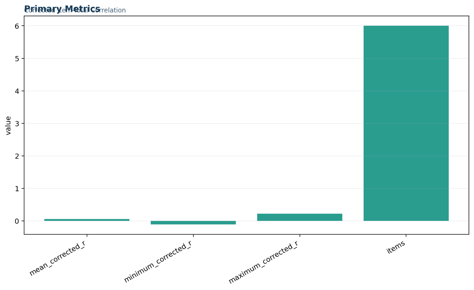
The Python chart set provides a visual audit of the Corrected Item-Total Correlation analysis. Figure 1 places the mean, minimum, maximum and item count in one summary. The maximum coefficient of 0.226597 and mean of 0.061453 immediately show that the proposed scale has weak internal item-rest alignment. The minimum of -0.104770 confirms that at least one item moves in the opposite direction from the remainder.
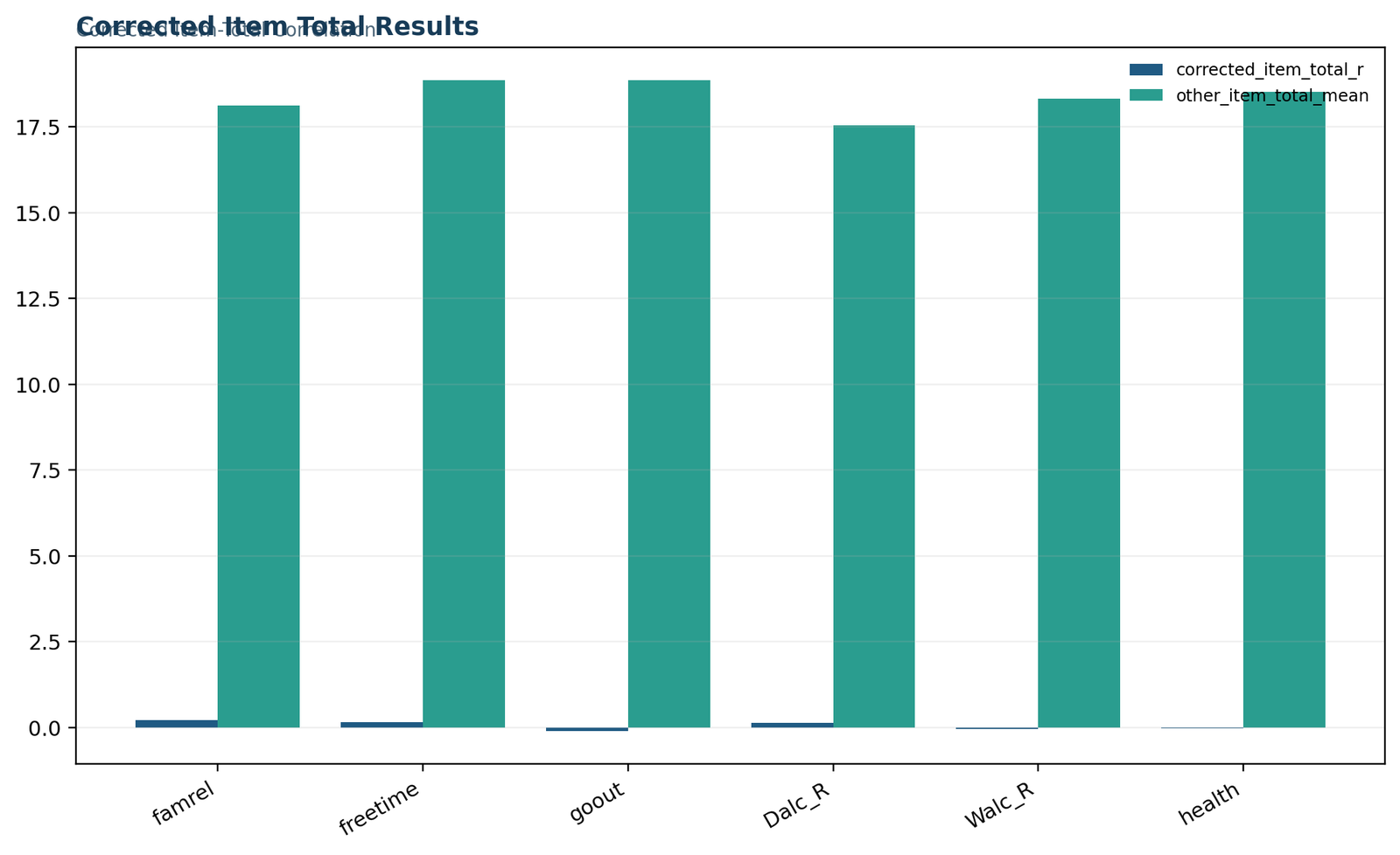
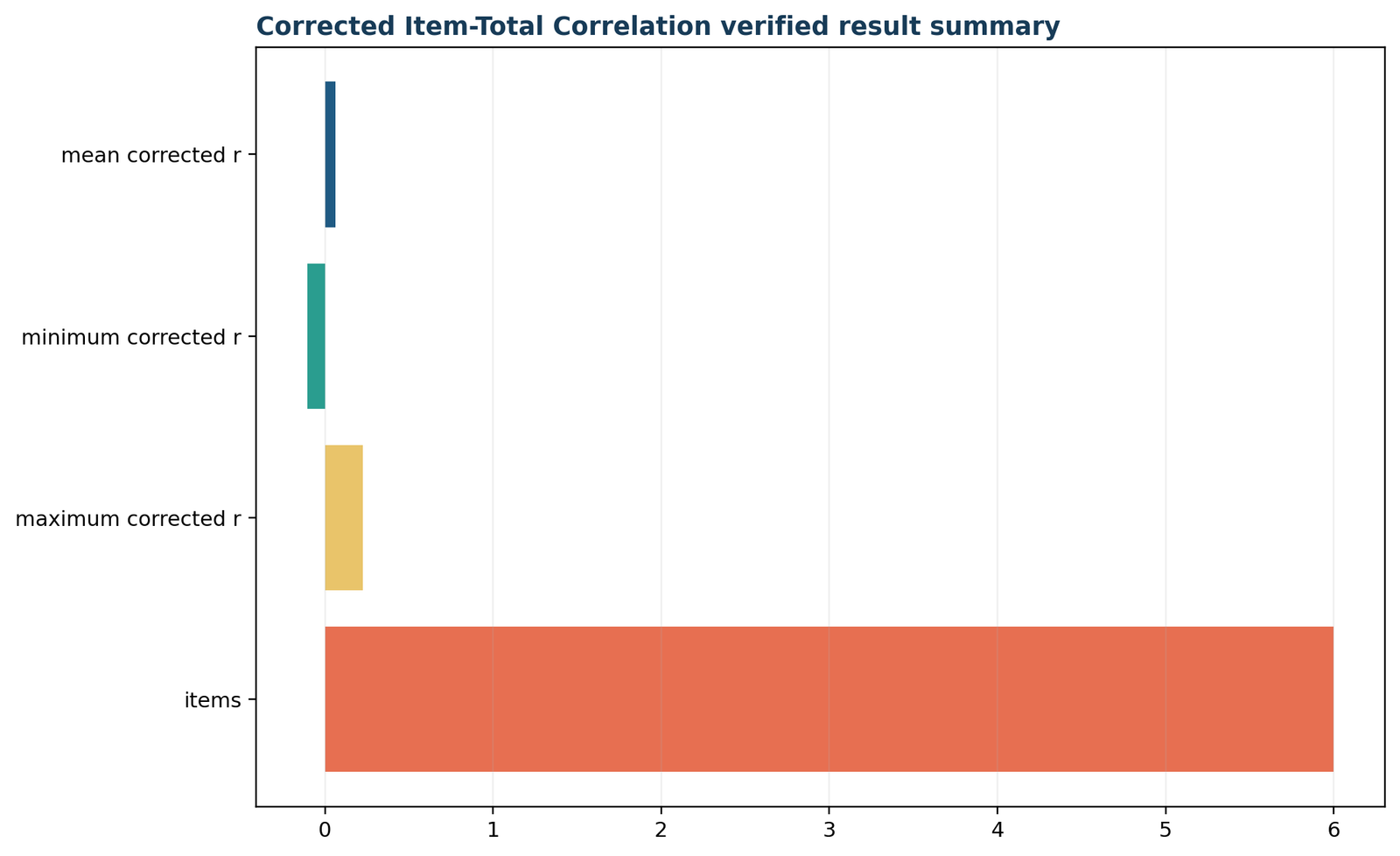
Python Figure 2 displays the six corrected coefficients directly. famrel ranks first, followed by freetime and Dalc_R. goout, Walc_R and health are negative. The plot is especially useful because it prevents the mean coefficient from hiding the mixed directions. A scale with one moderate positive item and several near-zero or negative items should not be summarized only by a single average.
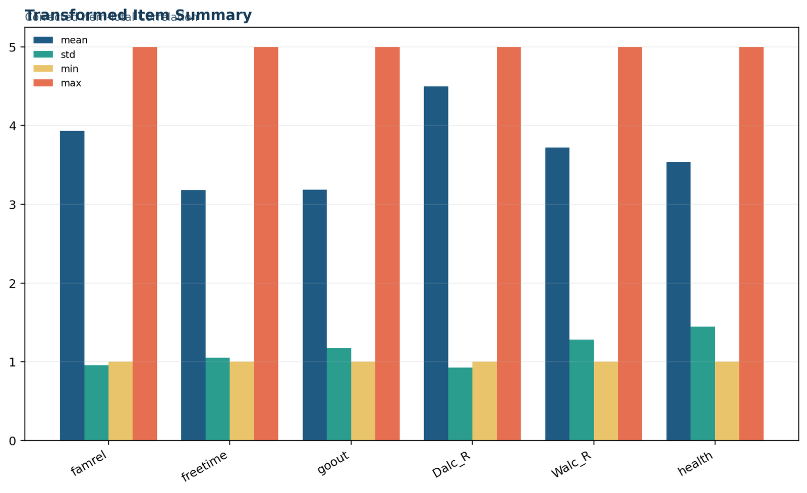
Python Figure 3 summarizes the transformed item distributions. It confirms that every item is on a 1-to-5 scale after reversing Dalc and Walc. The means and standard deviations show substantial differences in location and spread. These differences are not errors, but they help explain why standardized alpha is somewhat higher than raw alpha. Standardizing equalizes variance while preserving the correlation structure.
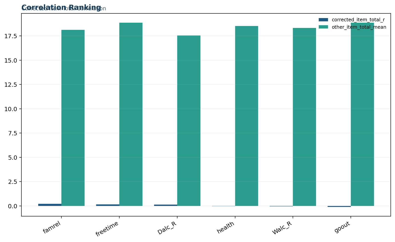
Python Figure 4 ranks the coefficients from highest to lowest. The ranking is a diagnostic priority list, not an automatic deletion list. The bottom item, goout, deserves coding and content review first. The next two negative items should also be examined, but their near-zero values may reflect conceptual separation rather than simple scoring mistakes. Figure 5 consolidates the result and confirms that the independent reference values match the calculated values.
The Python workflow uses each item as a target, creates a total from the other five items and applies Pearson correlation. It also exports CSV tables and a PDF report. Readers who need a broader explanation of the correlation function can continue to the correlation in Python guide. The public figures should be interpreted with the tables rather than treated as decorative graphics.
Corrected Item-Total Correlation R Charts
The R figures independently reproduce the same item-rest ordering and reliability conclusion.
The R chart set validates the Corrected Item-Total Correlation results with a separate implementation. Independent software agreement is important because it helps detect coding errors, omitted transformations and accidental use of an ordinary item-total correlation. The R workflow constructs the same six transformed items, excludes each target from its rest score and reports the same mean, minimum, maximum and ranking.
R Figure 1 confirms that the overall corrected-coefficient profile is weak. R Figure 2 shows the item-level coefficients and reproduces the positive values for famrel, freetime and Dalc_R, together with the negative values for goout, Walc_R and health. R Figure 3 confirms the means, standard deviations, minima and maxima of the transformed items.
R Figure 4 places the items in descending coefficient order. The ranking is identical to Python, which is the expected result when both programs use complete cases and Pearson correlation. R Figure 5 reports the final reference values and confirms the cross-check. The agreement between R, Python and SPSS indicates that the low reliability pattern comes from the data and scale definition, not from one software package.
R users can reproduce the calculation with cor(item, rowSums(scale[-item])) inside a loop or an lapply expression. The key is to remove the target column for each iteration. The correlation in R guide provides additional guidance on Pearson, Spearman and Kendall functions. For ordinal item analysis, analysts may compare Pearson and Spearman results, but they should state the chosen coefficient clearly rather than mix methods silently.
The R and Python figures are intentionally interpreted separately because software validation is part of the evidence. They do not change the substantive decision: the strongest Corrected Item-Total Correlation is only 0.226597, the average is 0.061453 and the six items should not be presented as a strong single internally consistent scale.
Calculate Corrected Item-Total Correlation in Python and R
The implementation should expose the rest-score construction rather than hide it inside an unexplained function.
In Python, load the item columns into a pandas DataFrame, reverse the necessary variables, and loop through the column names. For each target, drop that column, sum the remaining columns row by row and apply scipy.stats.pearsonr. Store the coefficient, p-value and rest-score mean in a results table. This direct implementation makes the Corrected Item-Total Correlation definition visible and auditable.
import pandas as pd
from scipy import stats

scale = pd.DataFrame({
    "famrel": df["famrel"],
    "freetime": df["freetime"],
    "goout": df["goout"],
    "Dalc_R": 6 - df["Dalc"],
    "Walc_R": 6 - df["Walc"],
    "health": df["health"]
})

rows = []
for item in scale.columns:
    rest_score = scale.drop(columns=item).sum(axis=1)
    r, p_value = stats.pearsonr(scale[item], rest_score)
    rows.append({"item": item, "corrected_r": r, "p_value": p_value})

results = pd.DataFrame(rows).sort_values("corrected_r", ascending=False)
In R, create a data frame with the transformed items, then iterate over the column positions. rowSums(scale[, -i]) forms the rest score and cor(scale[[i]], rest_score) calculates the coefficient. Use cor.test when a p-value or confidence interval is required. The same complete-case rule must be used in both the target item and rest score.
scale <- data.frame(
  famrel = data$famrel,
  freetime = data$freetime,
  goout = data$goout,
  Dalc_R = 6 - data$Dalc,
  Walc_R = 6 - data$Walc,
  health = data$health
)

result <- do.call(rbind, lapply(seq_along(scale), function(i) {
  rest_score <- rowSums(scale[, -i, drop = FALSE])
  data.frame(
    item = names(scale)[i],
    corrected_r = cor(scale[[i]], rest_score),
    rest_mean = mean(rest_score)
  )
}))
After calculating Corrected Item-Total Correlation, compute Cronbach’s alpha from the same scoring matrix and compare alpha if each item is deleted. The software outputs should be stored with full precision and rounded only for presentation. Reproducible scripts should also save the transformed data, item-level table, correlation ranking and run manifest. This prevents a later report from relying on copied values without a traceable calculation.
Python and R should produce the same coefficients when they use the same rows, transformations and Pearson formula. A mismatch usually means that one script handled missing data differently, included the target item in the total, used a different reverse-scoring constant or standardized the data at a different stage. Cross-software reconciliation should therefore compare input N, item names, scoring direction, coefficient order and full-precision values.
Corrected Item-Total Correlation in SPSS
The Item-Total Statistics table contains the corrected coefficient and alpha-if-deleted diagnostics.
In SPSS, place the six scored items into Analyze → Scale → Reliability Analysis. Choose the alpha model and request item, scale, scale-if-item-deleted and correlation statistics. The resulting Reliability Statistics table reports raw alpha, standardized alpha and the number of items. The Item-Total Statistics table reports the Corrected Item-Total Correlation for each item, together with scale mean if item deleted, scale variance if item deleted, squared multiple correlation and Cronbach’s alpha if item deleted.
The worked SPSS output uses 649 valid cases and excludes none. Raw alpha is .112, standardized alpha is .169 and the scale contains six items. The rounded corrected coefficients are .227 for famrel, .151 for freetime, -.105 for goout, .139 for Dalc_R, -.033 for Walc_R and -.010 for health. These match the full-precision Python and R calculations.
Read the SPSS table row by row. A positive corrected coefficient means the item is aligned with the rest score; a negative value is a warning. Then compare alpha if deleted with the overall alpha. Deleting goout raises alpha from .112 to .234, the largest change. Deleting famrel or freetime produces negative alpha values because the remaining average covariance becomes negative. SPSS attaches a footnote explaining this condition and recommending a coding check.
The SPSS correlation output provides an additional manual confirmation for selected items. For example, famrel correlated with its explicitly computed rest score at .227, freetime at .151 and goout at -.105. This separate correlation matrix is useful when teaching the method because it shows exactly what the reliability procedure is calculating. The correlation in SPSS guide explains how to read Pearson correlation rows, significance values and valid N.
SPSS should display .000 for very small significance values, but the written report should use p < .001 rather than p = .000. More importantly, do not let statistical significance replace the reliability decision. With N = 649, the weak positive coefficients can be significant while remaining inadequate for a strong scale.
Corrected Item-Total Correlation in Excel
A formula-driven workbook can reproduce every item-rest total and correlation without hidden calculations.
Arrange respondents in rows and scored items in columns. Add a full total column with =SUM(item cells). For each item, calculate a rest score as full total - target item. Then use =CORREL(target item range, rest score range). This produces the same Corrected Item-Total Correlation as Python, R and SPSS when the same complete rows are used.
| Excel task | Formula pattern | Purpose |
|---|---|---|
| Reverse a 1-to-5 item | =6-original_cell | Aligns a negatively directed item |
| Full score | =SUM(B2:G2) | Creates the six-item row total |
| Rest score for item B | =H2-B2 | Removes the target item from its total |
| Corrected coefficient | =CORREL(B$2:B$650,I$2:I$650) | Correlates target with its rest score |
| Item mean | =AVERAGE(B$2:B$650) | Checks location |
| Item SD | =STDEV.S(B$2:B$650) | Checks variation |
| Rank coefficients | =RANK.EQ(result,all_results,0) | Orders strongest to weakest |
Use separate rest-score columns or calculate each rest score directly from the other item columns. The full-total-minus-item approach is easier to audit. Ensure that the formula excludes the header row and covers exactly the 649 respondent rows. If blank cells exist, CORREL and row totals can handle them differently from SPSS listwise deletion, so create an explicit complete-case flag or filter to match the chosen missing-data rule.
The worked Excel file includes raw data, transformed items, item-rest calculations, summary values and a ranking table. It should show the same maximum of 0.226597, minimum of -0.104770 and mean of 0.061453. A conditional-formatting rule can highlight negative coefficients and values below 0.30, but the colors should support interpretation rather than replace it.
Excel is useful for teaching and auditing Corrected Item-Total Correlation because every row formula can be inspected. For final psychometric work, use software that also supports factor analysis, ordinal reliability, confidence intervals and robust missing-data methods. The workbook remains valuable as a transparent cross-check and as a reusable calculator for small item sets.
Corrected Item-Total Correlation Calculator Logic
A reliable calculator must remove the target item, validate the matrix and explain the result rather than display one number.
A Corrected Item-Total Correlation calculator should accept a rectangular respondent-by-item matrix. It should require at least two items and enough complete rows to calculate a correlation. The interface should let the analyst identify reverse-scored items, specify the minimum and maximum response values and choose a missing-data rule. Before calculation, it should reject nonnumeric values, constant items and rows that do not contain the required number of valid responses.
For each item, the calculator forms a rest score from all other items and calculates the selected correlation. The primary output should include the item name, coefficient, sample size, optional p-value, rank, threshold flag and alpha if deleted. Summary output should include the number of items, overall alpha, standardized alpha, mean coefficient, minimum coefficient and maximum coefficient. The full inter-item matrix is also useful because it explains why an item-rest value is weak or negative.
The calculator should not label every value below 0.30 as invalid. It should use wording such as ‘below the selected screening threshold; review theory, coding and dimensionality.’ Negative values should trigger a stronger warning to verify direction and item content. Very high values should prompt a redundancy check. This interpretation logic prevents users from deleting items mechanically.
To verify the calculator, test a small matrix where one item is identical to the sum pattern of the others, a matrix with one reverse-coded item, a matrix with a constant column and the 649-row worked dataset. The worked reference outputs are mean = 0.0614525980, minimum = -0.1047699380, maximum = 0.2265973305 and items = 6. A correct implementation should reproduce these values within floating-point tolerance.
Related browser tools are available in the statistical calculators collection. The calculator result should always be accompanied by the formula, item-level table and a short explanation of the measurement limitations. A downloadable CSV is useful for archiving the results, but the raw item data should remain protected when the matrix contains sensitive responses.
How to Make Item Decisions from Corrected Item-Total Correlation
Retain, revise, move or remove an item only after combining statistical and substantive evidence.
Begin with a scoring audit. Confirm the item wording, response anchors, reverse-scoring rule and valid range. A negative Corrected Item-Total Correlation caused by a coding mistake should be corrected and recalculated before any item decision. Next, inspect the frequency distribution, mean and standard deviation. An item with almost no variation may need better response options or a more discriminating wording.
Then inspect the inter-item matrix and factor structure. If an item correlates well with a subset of items but poorly with the total, it may belong to a subscale. Moving an item to a theoretically coherent subscale is often better than deleting it. If the item represents an essential content domain, revision may preserve validity better than removal. If the item is ambiguous or double-barreled, rewrite it and collect new pilot data rather than relying on a numerical adjustment.
Compare the Corrected Item-Total Correlation with alpha if deleted, but interpret both in context. In the worked data, removing goout increases alpha to 0.234. That change identifies a source of negative covariance but does not solve the scale. The item set still mixes family, leisure, social, alcohol-use and health content. A stronger redesign would specify a narrower construct and develop several items for each intended dimension.
Evaluate subgroup stability when the score will be used across populations. An item may show acceptable alignment overall but behave differently across sex, school, language or age groups. Differential item functioning and measurement invariance require methods beyond Corrected Item-Total Correlation, yet the item-rest pattern can guide which items deserve further investigation.
Finally, document the decision. Record the original coefficient, coding check, distribution, alpha if deleted, factor evidence, content rationale and action taken. Possible actions include retain unchanged, retain with monitoring, revise wording, reverse score, move to another subscale, remove from the total or collect more data. A transparent decision table is more defensible than a rule that deletes every item below 0.30.
How to Report Corrected Item-Total Correlation, Download the Files and Continue the Analysis
A complete report states the item set, sample, scoring, coefficients, alpha results and measurement decision.
A concise results paragraph should state that Corrected Item-Total Correlation was calculated by correlating each item with the sum of the remaining items. Report the number of respondents, number of items, range of coefficients, notable negative values, overall alpha and the practical conclusion. Do not report only the strongest coefficient, and do not describe statistically significant weak coefficients as strong.
An expanded report should explain that weekday and weekend alcohol-use items were reverse scored, list the item means and standard deviations, describe the inter-item matrix and note that the content spans several domains. If item deletion is discussed, state that the decision considered theory and dimensionality rather than alpha alone. The hypothesis testing guide and effect size guide can help distinguish inferential decisions from practical magnitude.
Download the complete analysis files
The PDF and Excel files provide the detailed software record behind the public interpretation. The Python and R reports reproduce the full-precision values and figures. The SPSS output contains Reliability Statistics, Item Statistics, the Inter-Item Correlation Matrix, Item-Total Statistics, Scale Statistics and selected manual correlation checks. The workbook provides formula-driven calculations for auditing.
Related Salar Cafe guides
These internal resources support the broader measurement workflow. Descriptive summaries explain item distributions; correlation guides explain the coefficient; reliability and agreement guides distinguish internal consistency from rater agreement; and calculator pages provide reusable browser tools. The final measurement decision should remain tied to the intended construct and use of the score.
Frequently Asked Questions About Corrected Item-Total Correlation
The answers address the most common definition, cutoff, SPSS, Excel and interpretation questions.
What does corrected item total correlation mean?
It means the correlation between one item and the score formed from all of the other items. The target item is removed from its comparison total so the coefficient is not inflated by self-inclusion. A positive Corrected Item-Total Correlation indicates that respondents with high item scores tend to have high rest scores.
What is an acceptable corrected item total correlation?
A commonly used screening benchmark is 0.30 or higher, but the acceptable value depends on the construct, scale length, development stage and intended use. Values from 0.20 to 0.29 may be retained provisionally with strong theoretical support. A Corrected Item-Total Correlation cutoff should guide review, not replace judgment.
Is 0.20 acceptable?
A coefficient around 0.20 is usually considered marginal. It may be acceptable during early exploratory development or for a content-essential item, but it should be reviewed with factor loadings, alpha if deleted, item wording and replication. In the worked data, the maximum Corrected Item-Total Correlation is 0.226597, yet the overall scale remains weak.
What does a negative corrected item-total correlation mean?
It means the item is inversely related to the rest score. Check reverse scoring, data entry, wording and construct membership. In this example, goout has Corrected Item-Total Correlation = -0.104770. The negative result is a meaningful diagnostic because it contributes negative covariance to the six-item total.
Should I delete every item below 0.30?
No. First verify coding, response range, item variance, content validity and dimensionality. An item may cover an important domain or belong to a different subscale. Deletion is justified only when statistical and substantive evidence support it.
What is the difference between item-total and corrected item-total correlation?
An ordinary item-total correlation includes the target item in the total, creating part-whole overlap. Corrected Item-Total Correlation removes the target item before calculating the total. The corrected coefficient is therefore the preferred item-rest diagnostic.
How is corrected item-total correlation related to Cronbach's alpha?
Both reflect item covariance. Corrected Item-Total Correlation is item specific, while alpha summarizes the complete item set. Alpha if item deleted shows how the overall coefficient changes when one item is removed. Neither statistic alone proves unidimensionality or validity.
Can corrected item-total correlation be statistically significant but unacceptable?
Yes. With a large sample, a small coefficient can have a very small p-value. In this dataset, some coefficients below 0.20 are statistically detectable because N = 649. Practical magnitude and measurement usefulness remain weak.
Where is corrected item-total correlation in SPSS?
Use Analyze → Scale → Reliability Analysis, place the scored items in the Items box, choose Model = Alpha, and request item, scale and scale-if-item-deleted statistics. SPSS displays the coefficient in the Item-Total Statistics table.
How do I calculate corrected item-total correlation in Excel?
Create the full row total, subtract the target item to create a rest score and use CORREL between the target-item column and rest-score column. Repeat for each item. Ensure that missing-data handling matches the intended analysis.
Can I use Spearman instead of Pearson?
Yes, when the item-rest relationship is monotonic, strongly ordinal or affected by nonlinearity and outliers. State the method explicitly. SPSS’s standard Corrected Item-Total Correlation column is based on Pearson-type covariance logic, so a Spearman analysis is an additional alternative rather than the same output.
What happens when an item has no variance?
A constant item cannot be correlated with a rest score because its standard deviation is zero. The coefficient is undefined. The item also cannot discriminate among respondents and should be reviewed or removed before reliability estimation.
Why is standardized alpha higher than raw alpha?
Standardized alpha is based on the correlation matrix and gives every item equal variance. Raw alpha uses the covariance matrix. In the worked example, unequal item variances and the correlation pattern produce raw alpha = 0.111763 and standardized alpha = 0.168910.
What does alpha if item deleted tell me?
It shows the internal-consistency coefficient for the remaining items after one item is removed. A higher value identifies an item that may be reducing alpha, but the resulting scale must still be theoretically coherent and sufficiently reliable.
Can a high corrected item-total correlation be too high?
An extremely high value may indicate redundancy, especially when several items use nearly identical wording. Strong alignment is useful, but the scale should cover the construct broadly rather than repeat the same question.
Does corrected item-total correlation prove validity?
No. It is evidence about internal item alignment. Validity also requires content evidence, response-process evidence, structural evidence, relations with external variables and consequences appropriate to the intended use.
How many respondents are needed?
There is no single universal minimum. Stability depends on the number of items, response distributions, expected coefficient and subgroup analyses. Larger samples provide more stable correlations. The worked example uses 649 complete records, so the weakness is unlikely to be explained only by a tiny sample.
Can I calculate it for binary items?
Yes. Pearson correlation between a binary item and a continuous rest score is a point-biserial correlation. For a full dichotomous test, KR-20 and item difficulty/discrimination analyses are also relevant.
Why is the mean corrected correlation not enough?
The mean can hide a mix of positive and negative items. In this example, the average is 0.061453, but the item values range from 0.226597 to -0.104770. The item-level table and matrix are necessary for diagnosis.
What is the final conclusion for this worked example?
None of the six items reaches 0.30, three coefficients are negative, raw alpha is 0.111763 and the best alpha after deletion is only 0.234087. The proposed total should be revised, divided into theoretically coherent subscales or replaced with a better item set.
Corrected Item-Total Correlation Conclusion and Methodological References
The coefficient is most useful when it leads to a transparent measurement decision rather than a mechanical cutoff.
Corrected Item-Total Correlation is a direct item-level test of whether one item moves with the score formed from the rest of a proposed scale. Its correction removes part-whole overlap and makes it more informative than an ordinary item-total correlation. Positive coefficients support common ordering, near-zero coefficients indicate weak linear alignment and negative coefficients signal opposite direction, coding problems or multidimensional content.
The worked analysis provides a clear diagnostic example. Across 649 complete records and six transformed items, the mean coefficient is 0.061453, the maximum is 0.226597 and the minimum is -0.104770. None reaches 0.30. Raw Cronbach’s alpha is 0.111763 and standardized alpha is 0.168910. Removing the most problematic item raises alpha only to 0.234087. Python, R, SPSS and Excel reproduce the same pattern.
The statistical evidence therefore does not support a dependable single six-item total. The content spans family relationship, leisure, social behavior, alcohol-use frequency and health. The correlation matrix contains both positive clusters and negative cross-domain relationships. The appropriate next step is to clarify the construct, review coding, consider subscales or factor analysis, revise the item pool and collect new pilot data. Reporting a total score without that work would attach a simple number to a measurement structure that the item analysis does not support.
The broader lesson is that an acceptable Corrected Item-Total Correlation is not a magic threshold. The coefficient should be interpreted with item variance, alpha if deleted, inter-item correlations, dimensionality, content coverage and intended use. Statistical significance can identify a nonzero relationship, but it cannot make a weak item practically strong. Transparent item decisions preserve both reliability and validity.
A useful sensitivity analysis recalculates Corrected Item-Total Correlation under plausible alternative scoring choices. For example, compare sums with means, Pearson with Spearman, complete cases with a prespecified partial-score rule, and the full scale with theoretically defined subscales. The purpose is not to search for the largest coefficient. It is to determine whether the item decision is stable when reasonable analytical choices change. If a coefficient changes direction under small scoring adjustments, the item is not providing robust evidence.
Researchers should also separate item quality from scale breadth. A broad construct can contain legitimate facets that correlate only moderately, while a narrow construct should usually show tighter item-rest alignment. Before applying a Corrected Item-Total Correlation cutoff, state whether the score is intended to represent a single narrow trait, a broad index or a formative combination. Reflective scales expect items to covary because they express a common latent variable. Formative indices combine components that need not correlate strongly, making internal-consistency screening less appropriate.
Sampling conditions can influence Corrected Item-Total Correlation. A homogeneous sample restricts variance and can reduce item-rest coefficients even when the item performs well in a broader population. A highly heterogeneous sample can increase correlations by widening score ranges. Replicate the item analysis in the target population and examine confidence intervals or bootstrap distributions when decisions are consequential. A coefficient should not be treated as a permanent property of an item independent of population and context.
Translation and cultural adaptation require special attention. An item may retain its literal meaning while losing its relationship with the construct in another language or setting. Cognitive interviews, expert review and subgroup analyses can identify why Corrected Item-Total Correlation changes across versions. Statistical revision should not remove culturally important content merely because a translated item has a lower coefficient in one pilot sample.
Response styles can also affect Corrected Item-Total Correlation. Acquiescence, extreme responding, straight-lining and socially desirable responding may create artificial associations or suppress genuine ones. Examine person-level response patterns, completion time and long strings when such data are available. A reliability coefficient cannot distinguish careful consistency from patterned responding without supporting quality checks.
For short scales, each item has a large effect on the rest score and alpha. A modest Corrected Item-Total Correlation may be unstable because the rest score contains only a few items. Report the number of items and avoid applying thresholds developed for longer instruments without qualification. Confidence intervals, bootstrap estimates and replication are particularly useful for short forms.
For ordinal Likert items, polychoric correlations and ordinal alpha or omega may better represent relationships among latent response tendencies. Pearson-based Corrected Item-Total Correlation remains common and interpretable, especially with five or more categories, but the analyst should recognize the measurement assumption. Comparing methods can show whether weak coefficients are caused by category coarseness or by genuine construct heterogeneity.
Item deletion changes the content domain. Removing a difficult, rare or negatively worded item may raise Corrected Item-Total Correlation and alpha while narrowing what the scale measures. Every deletion should be checked against the construct blueprint. A balanced instrument sometimes retains an item with a lower coefficient because it represents a necessary facet not covered elsewhere. The final report should make that rationale explicit.
After revision, collect new data rather than reporting coefficients calculated on the same sample used to select items as final evidence. Item selection capitalizes on sample-specific variation. Cross-validation in an independent sample provides a more honest estimate of Corrected Item-Total Correlation, alpha and factor structure. When an independent sample is not available, bootstrap stability and split-sample checks are useful but should be described as internal validation.
The strongest practical workflow combines statistics with traceable documentation. Preserve the original item wording, scoring key, transformation code, analysis script, software output and decision log. This record allows another analyst to reproduce every Corrected Item-Total Correlation value and understand why an item was retained, revised or removed. Reproducibility is part of measurement quality, not merely a technical convenience.
Corrected Item-Total Correlation remains the central definition diagnostic because it tests the target item against a total that excludes that item. Corrected Item-Total Correlation remains the central formula diagnostic because it tests the target item against a total that excludes that item. Corrected Item-Total Correlation remains the central interpretation diagnostic because it tests the target item against a total that excludes that item. Corrected Item-Total Correlation remains the central cutoff diagnostic because it tests the target item against a total that excludes that item. Corrected Item-Total Correlation remains the central SPSS output diagnostic because it tests the target item against a total that excludes that item. Corrected Item-Total Correlation remains the central Python calculation diagnostic because it tests the target item against a total that excludes that item. Corrected Item-Total Correlation remains the central R calculation diagnostic because it tests the target item against a total that excludes that item. Corrected Item-Total Correlation remains the central Excel formula diagnostic because it tests the target item against a total that excludes that item. Corrected Item-Total Correlation remains the central negative value diagnostic because it tests the target item against a total that excludes that item. Corrected Item-Total Correlation remains the central Cronbach’s alpha diagnostic because it tests the target item against a total that excludes that item. Corrected Item-Total Correlation remains the central item deletion diagnostic because it tests the target item against a total that excludes that item. Corrected Item-Total Correlation remains the central scale development diagnostic because it tests the target item against a total that excludes that item. Corrected Item-Total Correlation remains the central reliability analysis diagnostic because it tests the target item against a total that excludes that item. Corrected Item-Total Correlation remains the central item-rest score diagnostic because it tests the target item against a total that excludes that item. Corrected Item-Total Correlation remains the central acceptable threshold diagnostic because it tests the target item against a total that excludes that item. Corrected Item-Total Correlation remains the central measurement validity diagnostic because it tests the target item against a total that excludes that item. Corrected Item-Total Correlation remains the central definition diagnostic because it tests the target item against a total that excludes that item. Corrected Item-Total Correlation remains the central formula diagnostic because it tests the target item against a total that excludes that item. Corrected Item-Total Correlation remains the central interpretation diagnostic because it tests the target item against a total that excludes that item. Corrected Item-Total Correlation remains the central cutoff diagnostic because it tests the target item against a total that excludes that item. Corrected Item-Total Correlation remains the central SPSS output diagnostic because it tests the target item against a total that excludes that item. Corrected Item-Total Correlation remains the central Python calculation diagnostic because it tests the target item against a total that excludes that item. Corrected Item-Total Correlation remains the central R calculation diagnostic because it tests the target item against a total that excludes that item. Corrected Item-Total Correlation remains the central Excel formula diagnostic because it tests the target item against a total that excludes that item. Corrected Item-Total Correlation remains the central negative value diagnostic because it tests the target item against a total that excludes that item. Corrected Item-Total Correlation remains the central Cronbach’s alpha diagnostic because it tests the target item against a total that excludes that item.
Corrected Item-Total Correlation interpretation checklist: Corrected Item-Total Correlation should use a total that excludes the target item. Corrected Item-Total Correlation should be reviewed with the item’s mean and standard deviation. Corrected Item-Total Correlation should be checked for negative direction before deletion. Corrected Item-Total Correlation should be compared with alpha if item deleted. Corrected Item-Total Correlation should be interpreted with the inter-item correlation matrix. Corrected Item-Total Correlation should be recalculated after any scoring correction. Corrected Item-Total Correlation should be replicated in the target population. Corrected Item-Total Correlation should not be treated as proof of validity. Corrected Item-Total Correlation should support a documented retain, revise, move or remove decision. Corrected Item-Total Correlation should be reported with the sample size, item set and scoring rule.
Methodological references
Cronbach, L. J. (1951). Coefficient alpha and the internal structure of tests. Psychometrika, 16, 297–334.
DeVellis, R. F., & Thorpe, C. T. (2021). Scale Development: Theory and Applications. Sage.
Nunnally, J. C., & Bernstein, I. H. (1994). Psychometric Theory. McGraw-Hill.
Clark, L. A., & Watson, D. (1995). Constructing validity: Basic issues in objective scale development. Psychological Assessment, 7, 309–319.
Streiner, D. L. (2003). Starting at the beginning: An introduction to coefficient alpha and internal consistency. Journal of Personality Assessment, 80, 99–103.
These references emphasize that internal consistency is part of scale development rather than a stand-alone certificate. The worked files apply that principle by preserving item-level coefficients, transformed values, alpha results, inter-item relationships and cross-software verification.