
Chi Square Test of Independence: Formula, Example, Calculator, Python, R, SPSS and Excel Guide
The Chi Square Test of Independence evaluates whether two categorical variables are associated in one population or sample. This complete guide explains the research design, hypotheses, expected-count formula, manual calculation, assumptions, residuals, Cramér’s V, continuity correction, calculator steps, APA reporting, seven Python charts, six paired R charts, SPSS output and a worked Excel analysis using 649 students.
Chi Square Test of Independence Model Overview
The Chi Square Test of Independence is a nonparametric test of association for two categorical variables measured on the same independent observational units. It compares observed cell counts in a contingency table with the counts expected when the variables are statistically independent.
What Question Does the Test Answer?
The worked analysis asks whether student internet access is associated with intention to pursue higher education. Both variables are binary: internet is coded no/yes and higher is coded no/yes. Every student contributes to exactly one of the four cells.
How the Model Works
Under independence, the expected count in a cell is determined entirely by its row total, column total and the grand total. The Chi Square Test of Independence adds the standardized squared discrepancies between observed and expected counts. A large statistic indicates that the observed joint distribution is difficult to reconcile with independence.
Worked Result at a Glance
The observed table contains 22 students with neither internet access nor higher-education intention, 129 without internet access who intended higher education, 47 with internet access who did not intend higher education, and 451 with both. Pearson’s test gives χ²(1) = 3.2115, p = .0731. Cramér’s V is .0703, indicating a very small association.
Why the Primary Finding Is Not “Almost Significant”
A p-value of .073 is above the prespecified .05 threshold. It can be described as limited or inconclusive evidence, but not as a statistically significant result. The effect estimate, confidence interval and design limitations remain more informative than relabelling the threshold.
Search-intent note: Throughout this guide, Chi Square Test of Independence refers to Pearson’s contingency-table procedure for one sample and two categorical variables. The same Chi Square Test of Independence formula is used in the calculator, Python, R, SPSS and Excel sections, while the design wording remains distinct from homogeneity and goodness-of-fit tests.
The Chi Square Test of Independence remains an association test even when one variable is a plausible exposure and the other is a plausible outcome.
Quick Answer: Chi Square Test of Independence Result
The Chi Square Test of Independence quick answer should be read with the effect size and row percentages, not as a p-value alone.
The primary Pearson Chi Square Test of Independence compares internet access with higher-education intention in one sample of 649 students.
Test Summary
- Procedure: Pearson Chi Square Test of Independence without continuity correction
- Table: 2 × 2
- Minimum expected count: 16.0539
- Expected cells below 5: 0
- Decision: fail to reject H0 at .05
Substantive Meaning
- Without internet: 129 of 151 intended higher education, 85.43%.
- With internet: 451 of 498 intended higher education, 90.56%.
- Risk difference: 5.13 percentage points.
- Risk ratio: 1.060.
- Odds ratio: 1.636, 95% CI [0.951, 2.816].
Table of Contents
- What is a Chi Square Test of Independence?
- Research question, hypotheses and data design
- When to use the test
- Formula and manual calculation
- Variables and data dictionary
- Assumptions and conditions
- Complete worked results
- Residuals and cell contributions
- Independence versus related tests
- Calculator workflow
- Seven Python charts
- Six R charts in paired rows
- Software workflows
- Expandable code
- Advanced interpretation
- APA reporting
- Common mistakes
- Practice problems
- AP Statistics notes
- Downloads
- Related guides
- Frequently asked questions
- Conclusion
What Is a Chi Square Test of Independence?
The Chi Square Test of Independence definition begins with the one-sample design because design determines the correct hypothesis language.
A Chi Square Test of Independence determines whether the distribution of one categorical variable changes across the categories of another categorical variable when both are recorded from one sample. The method works with frequencies, not means, medians or individual numerical measurements.
Independence in Plain Language
Two variables are independent when knowing a person’s category on one variable does not change the probability distribution of the other. In this example, independence would mean that the proportion intending higher education is the same among students with and without internet access.
Association Is the Alternative
The alternative hypothesis says that the variables are associated. Association means the conditional proportions differ somewhere in the table. It does not automatically establish a direct causal mechanism, and it does not say which variable causes the other.
What the Statistic Measures
The test statistic is a weighted distance between the observed table and the table predicted by independence. Squaring prevents positive and negative deviations from cancelling. Dividing by the expected count expresses each discrepancy relative to the size of its cell.
What the Test Does Not Tell You
- It does not prove causation.
- It does not identify the strongest cell without residual analysis.
- It does not quantify practical importance without an effect size.
- It does not adjust for age, school, socioeconomic status or other covariates.
- It does not make repeated or clustered observations independent.
Common Table Sizes
The procedure is not limited to a 2 × 2 table. It can analyse a 2 × 3, 4 × 5 or other r × c contingency table, provided the observations are independent and expected counts are adequate. The degrees of freedom increase as (r − 1)(c − 1).
Research Question, Hypotheses and Data Design
The Chi Square Test of Independence research question must name both categorical variables and the population represented by the sample.
The Chi Square Test of Independence alternative is nondirectional unless a separate planned contrast is specified.
internet: no or yes.higher: no or yes.Research Question
Is internet access associated with intention to pursue higher education among the students represented in the analysed dataset?
Hypotheses
| Hypothesis | Statistical statement | Meaning |
|---|---|---|
| Null hypothesis | H0: internet ⟂ higher | The conditional distribution of higher-education intention is the same at each internet-access level. |
| Alternative hypothesis | H1: internet is associated with higher | At least one conditional proportion differs. |
| Decision rule | Reject H0 when p < α | The α level must be selected before viewing the result. |
Sampling Design Statement
The same student sample supplies both variables. The study does not contain one independently sampled population of students without internet and a second independently sampled population with internet. That difference is why the analysis is described as a Chi Square Test of Independence rather than a homogeneity test.
Direction and Causality
The Pearson chi-square statistic is nondirectional. It can detect that the row profiles differ but does not itself label the direction. Direction comes from the observed percentages, residual signs and effect measures. Because the data are observational, even a significant result would not prove that internet access causes higher-education intention.
When to Use a Chi Square Test of Independence
The Chi Square Test of Independence is appropriate only when the variables, observations and frequency structure meet the conditions below.
Use the Test When
- Two variables are categorical.
- Both variables are observed on the same units.
- The observations are independent.
- The data are frequencies in mutually exclusive cells.
- The research question concerns association or independence.
- Expected counts are sufficiently large for the chi-square approximation.
Choose Another Method When
- The same people are measured twice in paired categories.
- Observations are clustered or repeatedly measured.
- A continuous outcome should remain continuous.
- Covariate-adjusted association is required.
- Cells are structurally impossible or expected counts are sparse.
- The goal is prediction, causal estimation or time-to-event modelling.
Test-Selection Flow
If no, choose a method for quantitative or mixed data.
If no, use a paired, repeated-measures or clustered method.
One sample supports independence wording; several populations support homogeneity wording.
Examples That Fit
- Smoking status by disease status in a cross-sectional sample.
- Preferred learning mode by year level in one student survey.
- Product category by payment method in one transaction dataset.
- Political preference by age group in one probability sample.
Examples That Do Not Fit
- Before-versus-after binary responses from the same participants: use McNemar’s test.
- Repeated ratings with more than two categories: consider a marginal homogeneity or symmetry procedure.
- Binary outcome with several predictors: use logistic regression.
- Two independent proportions with sparse cells: consider Fisher, Barnard or Boschloo according to design.
Chi Square Test of Independence Formula and Manual Calculation
The Chi Square Test of Independence calculation can be audited cell by cell from observed counts through the final p-value.
The manual Chi Square Test of Independence calculation begins with the observed table, derives expected counts from the margins, computes one contribution per cell and adds those contributions.
Step 1: Observed Counts
| Internet access | Higher: no | Higher: yes | Row total |
|---|---|---|---|
| No | 22 | 129 | 151 |
| Yes | 47 | 451 | 498 |
| Column total | 69 | 580 | 649 |
Step 2: Expected-Count Formula
For the no-internet/no-higher cell:
Step 3: Expected Counts
| Internet access | Higher: no | Higher: yes |
|---|---|---|
| No | 16.053929 | 134.946071 |
| Yes | 52.946071 | 445.053929 |
Step 4: Cell Contributions
| Cell | Observed O | Expected E | O − E | (O − E)²/E |
|---|---|---|---|---|
| No internet, no higher | 22 | 16.053929 | +5.946071 | 2.202312 |
| No internet, yes higher | 129 | 134.946071 | −5.946071 | 0.261999 |
| Internet, no higher | 47 | 52.946071 | −5.946071 | 0.667769 |
| Internet, yes higher | 451 | 445.053929 | +5.946071 | 0.079442 |
Step 5: Degrees of Freedom
Step 6: P-Value and Decision
For χ² = 3.211522 with 1 degree of freedom, p = .073121. Since .073121 > .05, the analysis fails to reject the null hypothesis of independence.
Why Every Deviation Has the Same Raw Magnitude
In a 2 × 2 table with fixed margins, the four observed-minus-expected deviations must appear as +d, −d, −d and +d. Their chi-square contributions differ because each is divided by a different expected count. The smallest expected cell therefore contributes the most.
Variables and Data Dictionary
The Chi Square Test of Independence variables must be coded as mutually exclusive categorical levels before the table is formed.
| Variable | Role | Coding | Counts | Meaning |
|---|---|---|---|---|
internet | Row categorical variable | no / yes | No = 151; Yes = 498 | Whether the student reported internet access. |
higher | Column categorical variable | no / yes | No = 69; Yes = 580 | Whether the student intended to pursue higher education. |
| Student | Observational unit | One row per student | N = 649 | Each student contributes to one and only one cell. |
| Cell frequency | Analysis input | Nonnegative integer count | 22, 129, 47, 451 | Observed number of students in each joint category. |
Observed Joint Distribution
| Internet access | Higher = no | Higher = yes | Total | Higher = yes row percentage |
|---|---|---|---|---|
| No | 22 | 129 | 151 | 85.430% |
| Yes | 47 | 451 | 498 | 90.562% |
| Total | 69 | 580 | 649 | 89.368% |
Conditional Percentages
The row percentages answer the substantive comparison. Among students without internet access, 14.57% did not intend higher education and 85.43% did. Among students with internet access, 9.44% did not intend higher education and 90.56% did.
Column Percentages
Among the 69 students who did not intend higher education, 31.88% lacked internet access and 68.12% had internet access. Among the 580 who intended higher education, 22.24% lacked internet access and 77.76% had internet access. Column percentages answer a different conditional question and should not be substituted for row percentages without explanation.
Chi Square Test of Independence Assumptions and Conditions
The Chi Square Test of Independence assumptions include independent observational units as well as adequate expected frequencies.
One student must not contribute multiple correlated records.
All four cells comfortably exceed five.
No missing cases in the two analysed fields.
Assumption 1: Count Data
The input must be frequencies. Percentages may be reported, but the test itself must be calculated from integer counts or equivalent weighted case frequencies.
Assumption 2: Mutually Exclusive Categories
Every student must fall into exactly one category for internet access and exactly one category for higher-education intention. Ambiguous or overlapping categories invalidate the table construction.
Assumption 3: Independent Observations
The independence assumption concerns observational units, not the relationship being tested. Students should be sampled or observed independently. Siblings, repeated student records or students nested in a small number of schools may create dependence that the ordinary chi-square reference distribution ignores.
Assumption 4: Expected Counts
A common rule is that no expected cell should be below 1 and no more than 20% should be below 5. More conservative courses require every expected count to be at least 5. Here the minimum is 16.0539, so the expected-count condition is satisfied under either rule.
Assumption 5: Appropriate Sampling and Generalization
The test can be computed from any complete table, but population inference requires a defensible sampling design. A convenience sample can describe the analysed students without automatically representing all students.
Assumption 6: Predefined Categories
Categories and cut points should be selected for substantive reasons rather than repeatedly changed until a preferred p-value appears. Data-driven recoding inflates false-positive risk.
Complete Chi Square Test of Independence Results
The Chi Square Test of Independence results combine the global statistic, conditional percentages, sensitivity checks and effect size.
The Chi Square Test of Independence sensitivity analyses are secondary checks rather than opportunities to select a preferred p-value.
Primary statistic
2 × 2 table
Two-sided asymptotic
Very small
No sparse cells
Sensitivity analysis
Primary and Sensitivity Tests
| Procedure | Statistic | df | P-value | Decision at .05 |
|---|---|---|---|---|
| Pearson chi-square, no correction | 3.211522 | 1 | 0.073121 | Fail to reject H0 |
| Yates continuity correction | 2.694122 | 1 | 0.100719 | Fail to reject H0 |
| Likelihood-ratio chi-square | 3.011 | 1 | 0.083 | Fail to reject H0 |
| Fisher’s exact test, two-sided | — | — | 0.096 | Fail to reject H0 |
| Fisher’s exact test, one-sided | — | — | 0.053 | Not prespecified as primary |
Supplementary 2 × 2 Effect Estimates
| Measure | Estimate | Approximate 95% CI | Interpretation |
|---|---|---|---|
| Higher-intention rate without internet | 0.854305 | — | 129 of 151 students. |
| Higher-intention rate with internet | 0.905622 | — | 451 of 498 students. |
| Risk difference, internet yes − no | 0.051318 | [−0.0105, 0.1132] | Observed difference of 5.13 percentage points. |
| Risk ratio | 1.060070 | [0.9867, 1.1389] | Higher-intention probability was about 6% higher in the internet group. |
| Odds ratio | 1.636484 | [0.9510, 2.8161] | Observed odds were higher, but the interval includes 1. |
| Cramér’s V / Phi | 0.070345 | — | Very small standardized association. |
Statistical Interpretation
The Pearson p-value is .0731. At α = .05, the result is not statistically significant. The data do not provide sufficient evidence to reject independence between internet access and higher-education intention.
Practical Interpretation
The observed intention rate was 90.56% for students with internet access and 85.43% for students without internet access. The 5.13-point difference may be descriptively interesting, but Cramér’s V = .070 indicates that the overall association is very small. The approximate risk-difference interval includes zero.
Consistency Across Methods
Pearson, Yates, likelihood-ratio and Fisher procedures all remain above .05. The conclusion is therefore not dependent on a single borderline correction choice. This consistency is more important than choosing the smallest p-value.
Cell Contributions, Residuals and Follow-Up Interpretation
The Chi Square Test of Independence diagnostics explain which cells lie above or below the independence model.
Pearson Residuals
| Internet access | Higher = no | Higher = yes |
|---|---|---|
| No | +1.484019 | −0.511859 |
| Yes | −0.817172 | +0.281854 |
A positive Pearson residual means more observations than expected under independence. A negative residual means fewer. None of the absolute Pearson residuals reaches 2, so no cell displays a conventionally large local discrepancy.
Adjusted Standardized Residuals
| Internet access | Higher = no | Higher = yes |
|---|---|---|
| No | +1.792072 | −1.792072 |
| Yes | −1.792072 | +1.792072 |
Adjusted residuals account for row and column proportions and are often interpreted approximately as standard normal scores. Their absolute magnitude of 1.79 remains below 1.96, consistent with the non-significant global result.
Cell Contributions
| Cell | Contribution | Share of total χ² |
|---|---|---|
| No internet, no higher | 2.202312 | 68.57% |
| No internet, yes higher | 0.261999 | 8.16% |
| Internet, no higher | 0.667769 | 20.79% |
| Internet, yes higher | 0.079442 | 2.47% |
The no-internet/no-higher cell contributes most because its observed count of 22 exceeds the expected count of 16.05 and because the expected count is relatively small. This does not mean that the cell is independently significant; contributions are descriptive components of the global statistic.
Post-Hoc Interpretation
For larger tables, analysts may inspect adjusted residuals with multiplicity correction. Here the 2 × 2 table has only one degree of freedom, and all four deviations express the same underlying association. Separate post-hoc cell tests are unnecessary.
Expected-Count Diagnostics
- Minimum expected count = 16.0539.
- Cells expected below 5 = 0.
- Proportion below 5 = 0%.
- No zero expected counts.
- Pearson approximation is numerically appropriate.
Chi Square Test of Independence Versus Homogeneity, Goodness of Fit and Other Tests
The Chi Square Test of Independence should be distinguished from procedures that answer different design-based questions.
One sample, two categorical variables, association question.
Several populations or groups, one categorical response distribution.
One categorical variable compared with specified probabilities.
Exact 2 × 2 analysis, especially when expected counts are sparse.
| Method | Data design | Null hypothesis | Typical table |
|---|---|---|---|
| Chi Square Test of Independence | One sample; two categorical variables | The variables are independent | r × c |
| Chi square test for homogeneity | Two or more populations/groups; one categorical response | Response distributions are identical | r × c |
| Chi square goodness-of-fit test | One categorical variable | Observed probabilities equal specified probabilities | 1 × k |
| Fisher’s exact test | Usually a sparse 2 × 2 table | Conditional odds ratio equals 1 | 2 × 2 |
| McNemar’s test | Paired binary outcomes | Discordant probabilities are equal | Paired 2 × 2 |
| Logistic regression | Binary outcome plus one or more predictors | Predictor coefficients equal zero | Row-level data |
Independence Versus Homogeneity
The formulas, expected counts and chi-square statistic can be identical. The difference lies in how the data were obtained and how the research question is framed. This worked dataset records both internet access and higher-education intention from one student sample, so independence language is correct.
Independence Versus Goodness of Fit
A goodness-of-fit test studies one categorical variable and compares it with externally specified or theoretically expected proportions. The present table contains two variables, and the expected counts are estimated from both sets of margins.
Independence Versus a Two-Proportion Z Test
For a 2 × 2 table, the uncorrected Pearson chi-square statistic equals the square of the pooled two-proportion z statistic. The tests give the same two-sided p-value. The z test highlights the difference between two proportions; the chi-square formulation generalizes more naturally to larger tables.
Independence Versus Fisher’s Exact Test
Fisher’s exact test conditions on the margins. Here all expected counts exceed 16, so Pearson’s approximation is suitable. Fisher’s two-sided p-value of .096 is reported as a sensitivity result rather than replacing the prespecified primary test.
Independence Versus Logistic Regression
Logistic regression is preferable when covariate adjustment, prediction, interactions or clustered extensions are required. A simple binary logistic model with higher as the outcome and internet as the predictor would estimate the same unadjusted odds ratio, but it offers a framework for adding confounders.
Chi Square Test of Independence Calculator: Step-by-Step Workflow
The Chi Square Test of Independence calculator workflow below provides exact checkpoints for all four cells.
The Chi Square Test of Independence calculator checks below also help detect transposed or mistyped tables.
A reliable Chi Square Test of Independence calculator requires the observed contingency table and should return expected counts, the Pearson statistic, degrees of freedom, p-value and preferably an effect size.
Calculator Inputs
Step 1: Preserve the Table Orientation
Rows should represent internet access and columns should represent higher-education intention. Swapping rows or columns does not change χ² or p, but it changes row percentages, residual signs and the direction of ratios.
Step 2: Confirm Margins
Row totals must be 151 and 498; column totals must be 69 and 580; N must be 649. An incorrect total means the table was transcribed incorrectly.
Step 3: Select Pearson Without Correction as Primary
For the main result, use Pearson χ² without Yates correction. The expected-count condition is satisfied. Report the correction only as a sensitivity analysis when required by a course or software default.
Step 4: Verify Expected Counts
The calculator should return 16.0539, 134.9461, 52.9461 and 445.0539. These values are determined by the margins, not supplied independently.
Step 5: Verify the Result
The target is χ² = 3.2115218, df = 1 and p = .0731214. Cramér’s V or phi should be .070345.
Step 6: Interpret More Than the P-Value
Compare row percentages, inspect residuals and report Cramér’s V. A calculator result that contains only “accept” or “reject” is insufficient for a complete analysis.
Python Chi Square Test of Independence Charts
The Chi Square Test of Independence Python charts translate the numerical output into seven connected visual explanations.
The Python workflow generates seven figures. Each chart is interpreted with exact values so the visual is not separated from the statistical result.
Chart 1: Observed CountsPython
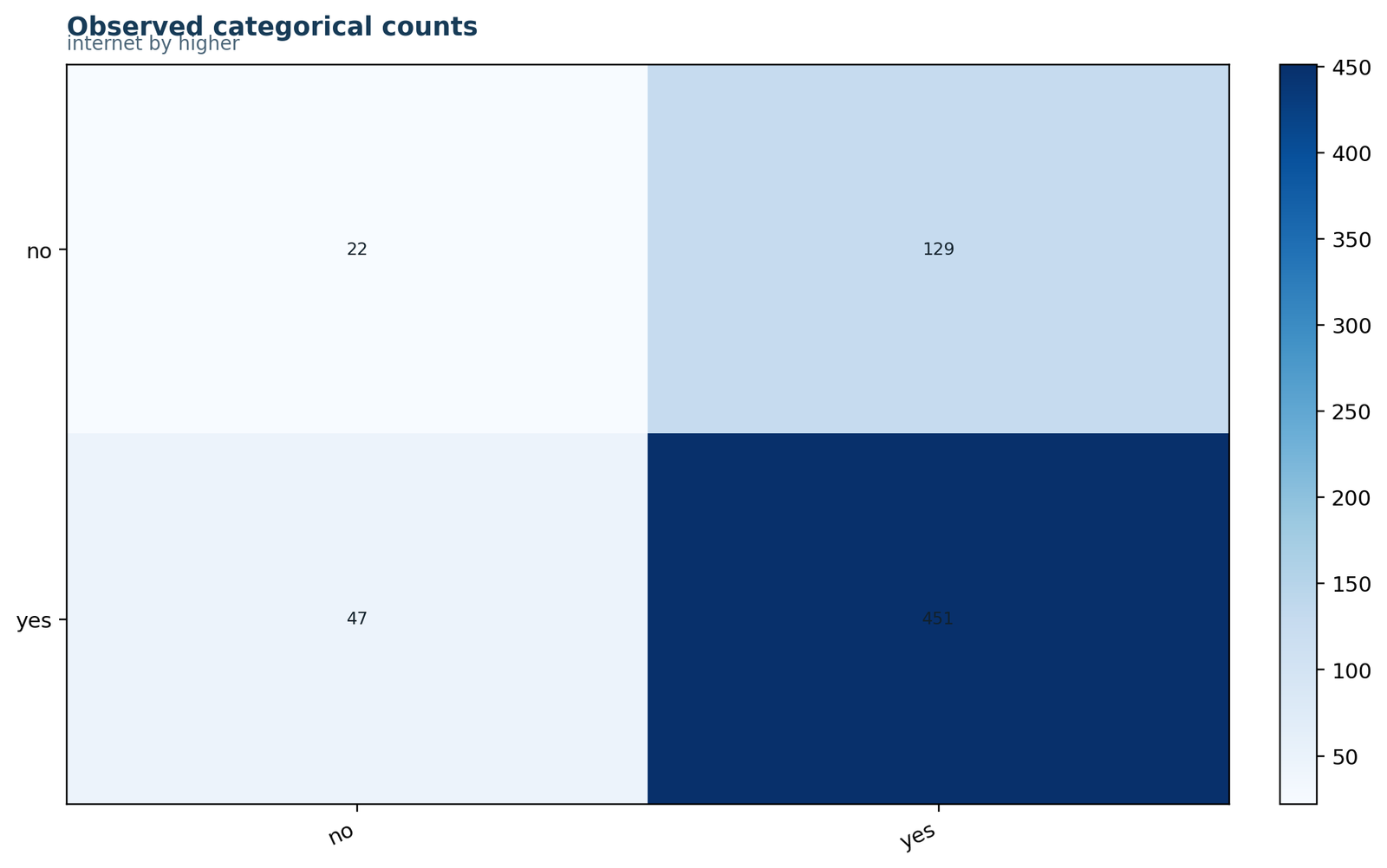
The largest cell contains students with internet access who intended higher education. The smallest cell contains students without internet access who did not intend higher education.
No internet: 22 no and 129 yes. Internet: 47 no and 451 yes. Row totals are 151 and 498.
Raw counts show the joint distribution but are strongly affected by unequal row totals. The internet-access group is more than three times larger.
The observed table is the starting point for all expected counts, percentages and effect estimates.
Chart 2: Expected Counts Under IndependencePython
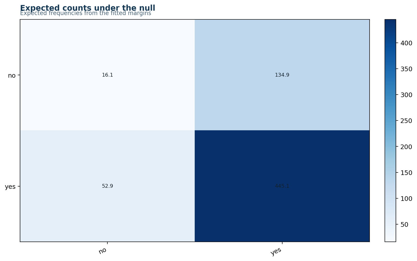
Expected counts retain the same row and column totals as the observed table. The no-internet/no-higher cell is expected to contain about 16.05 students.
Expected counts: 16.0539, 134.9461, 52.9461 and 445.0539. Minimum expected = 16.0539.
The observed no-internet/no-higher count is 5.95 above expectation; the internet/no-higher count is 5.95 below expectation.
Expected counts define the comparison model. Their adequacy also determines whether the Pearson approximation is appropriate.
Chart 3: Pearson ResidualsPython
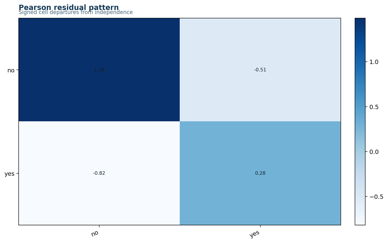
The strongest positive residual is in the no-internet/no-higher cell. The strongest negative residual is in the internet/no-higher cell.
Residuals: +1.4840, −0.5119, −0.8172 and +0.2819. None has |residual| ≥ 2.
The residual signs indicate that students without internet appear somewhat more often than expected in the no-higher category, but the deviations are not individually large.
The global p-value does not show which cells create the statistic. Residuals provide that local explanation.
Chart 4: Cell Contributions to Pearson Chi-SquarePython
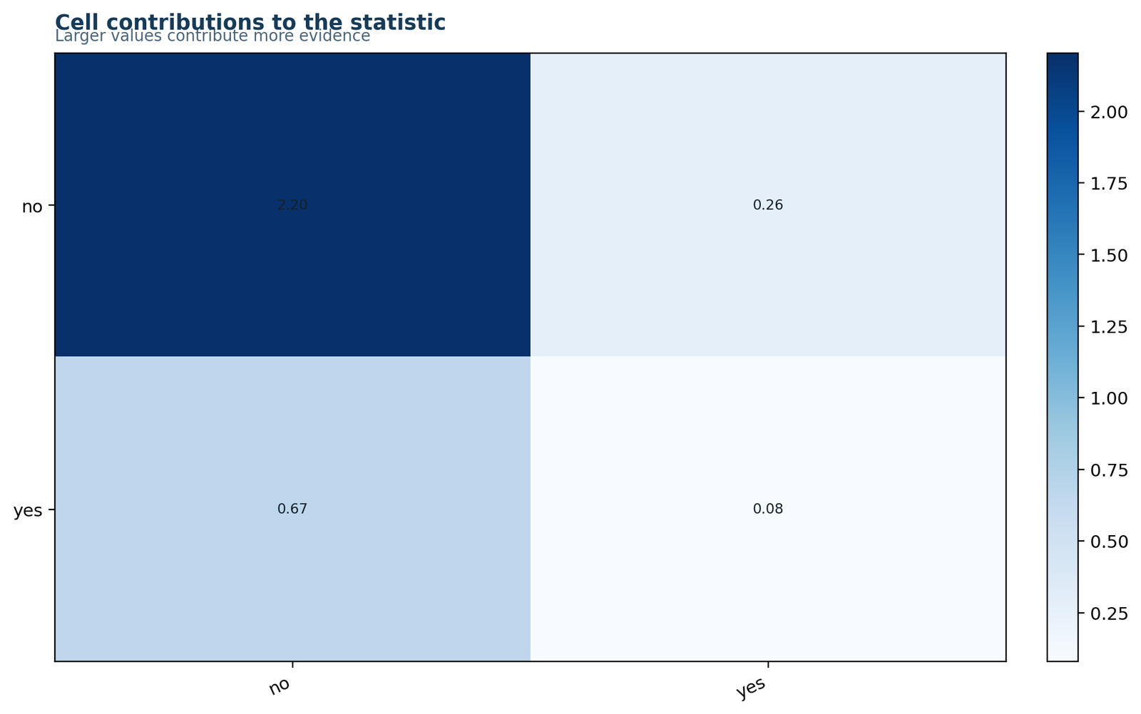
The no-internet/no-higher cell dominates the statistic, followed by the internet/no-higher cell.
Contributions: 2.2023, 0.2620, 0.6678 and 0.0794; total = 3.2115. The first cell contributes 68.57%.
A large contribution means that a cell has a relatively large observed-to-expected discrepancy, not that the cell is a separate hypothesis test.
Contribution analysis prevents vague statements that the whole table differs uniformly.
Chart 5: Within-Internet Row PercentagesPython
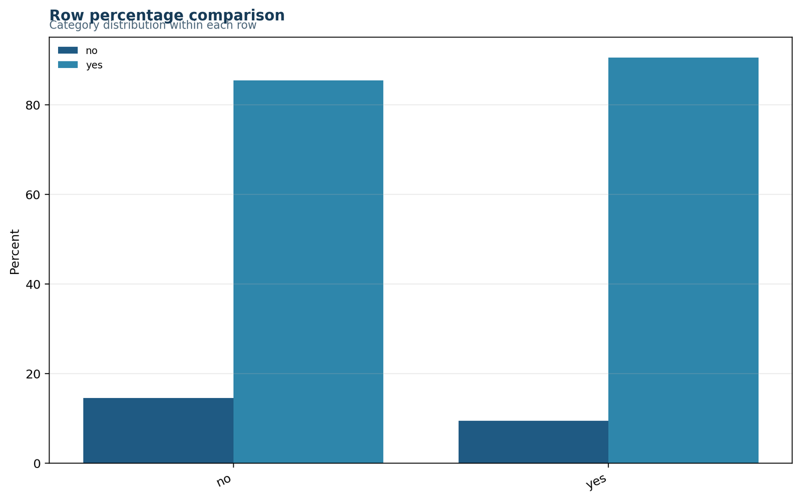
The higher-education intention segment is larger among students with internet access.
Higher intention: 85.43% without internet and 90.56% with internet. Difference = 5.13 percentage points.
The descriptive difference favours the internet-access group, but the inferential result is p = .073 and the effect is very small.
Percentages answer the substantive question more directly than raw counts when row totals differ.
Chart 6: Model DiagnosticsPython
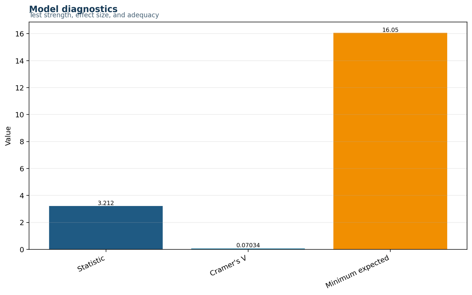
The expected-count condition is comfortably satisfied, while the effect-size bar remains close to zero.
N = 649; df = 1; minimum expected = 16.0539; cells below 5 = 0; Cramér’s V = 0.0703.
The chi-square approximation is suitable. The small effect size shows that a non-significant p-value is not hiding a large observed association.
Diagnostics distinguish a valid null result from an inconclusive result caused by sparse cells.
Chart 7: Pearson Versus Continuity-Corrected ResultPython
P-values are scaled from 0 to .12. Both results remain above the α = .05 decision threshold.
Yates correction reduces the statistic and increases the p-value, as expected for a continuity adjustment.
Pearson: χ² = 3.2115, p = .0731. Yates: χ² = 2.6941, p = .1007.
Neither method rejects at .05. The correction affects the numerical strength but not the conclusion.
Software defaults differ, so analysts must state whether correction was applied.
R Chi Square Test of Independence Chart Pairs
The Chi Square Test of Independence R charts reproduce the same verified counts and statistics in three paired rows.
The R section presents six figures in three paired rows. Each chart has a dedicated explanation box, matching the permanent post layout.
The R count heatmap reproduces 22, 129, 47 and 451. It confirms the exact contingency table used by the test.
The expected table is 16.0539, 134.9461, 52.9461 and 445.0539. Every expected frequency exceeds five.
The largest absolute Pearson residual is +1.4840 in the no-internet/no-higher cell. None reaches ±2.
The no-internet/no-higher cell contributes 2.2023 of the total 3.2115, or 68.57%.
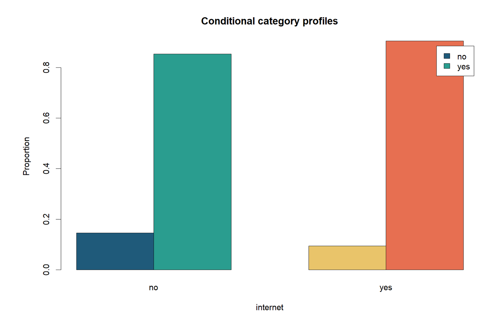
R summary: minimum expected count = 16.0539; expected cells below five = 0.
Higher-education intention is 85.43% without internet and 90.56% with internet. The descriptive gap is 5.13 points.
The R summary reports χ² = 3.2115, df = 1, p = .0731, Cramér’s V = .0703 and minimum expected = 16.0539.
Chi Square Test of Independence in Python, R, SPSS, Excel and Other Software
The Chi Square Test of Independence software workflow must preserve table orientation and correction settings across programs.
Chi Square Test of Independence in Python
Use scipy.stats.chi2_contingency with correction=False for the primary Pearson result. Preserve row and column labels separately because the numeric array alone does not retain their meanings.
- Build the 2 × 2 count table.
- Run Pearson without correction.
- Save expected counts, residuals and contributions.
- Calculate Cramér’s V.
- Run Yates and Fisher only as declared sensitivity checks.
Chi Square Test of Independence in R
Create a labelled matrix and use chisq.test(tab, correct = FALSE). The returned object contains observed counts, expected counts, Pearson residuals, statistic, degrees of freedom and p-value.
- Use
prop.table(tab, 1)for row profiles. - Square residuals for cell contributions.
- Use
fisher.test(tab)for an exact sensitivity result. - Report the correction setting.
Chi Square Test of Independence in SPSS
Use Analyze → Descriptive Statistics → Crosstabs. Put internet in rows and higher in columns. Request Chi-square and Phi/Cramér’s V, then request counts, expected counts, row percentages and standardized residuals.
- Pearson χ² = 3.212, p = .073.
- Continuity correction = 2.694, p = .101.
- Fisher two-sided p = .096.
- Phi and Cramér’s V = .070.
Chi Square Test of Independence in Excel
Excel can calculate margins, expected counts, contributions and the p-value. Use CHISQ.DIST.RT for a statistic-based result or CHISQ.TEST with observed and expected ranges.
- Expected = row total × column total ÷ grand total.
- Contribution = (observed − expected)² ÷ expected.
- df = (rows − 1)(columns − 1).
- Cramér’s V = SQRT(χ²/(N × MIN(r−1,c−1))).
TI-84 and TI-Nspire
Enter observed counts in a matrix, run the χ²-Test command and store the expected matrix. Confirm that the calculator reports χ² ≈ 3.212, p ≈ .0731 and df = 1.
- Do not enter row percentages as counts.
- Check matrix dimensions.
- Round only after the final result.
StatCrunch, Minitab, Jamovi and JASP
Choose a contingency-table analysis, select row and column variables, and request expected counts, row percentages, residuals and association measures.
- Verify whether continuity correction is enabled.
- Check the test label and sampling design.
- Export the full output, not only the p-value.
SAS
Use PROC FREQ with a two-way table and the CHISQ option. Add EXPECTED, DEVIATION and cell-percentage options as needed.
Stata
Use tabulate internet higher, chi2 expected row. Add exact options for a 2 × 2 sensitivity analysis when needed.
Expandable Chi Square Test of Independence Code
The Chi Square Test of Independence code examples use the same observed table so every platform can be cross-checked.
Python code
import numpy as np
from scipy.stats import chi2_contingency, fisher_exact

observed = np.array([[22, 129],
                     [47, 451]])

chi2, p_value, df, expected = chi2_contingency(
    observed, correction=False
)
residuals = (observed - expected) / np.sqrt(expected)
contributions = (observed - expected) ** 2 / expected
n = observed.sum()
cramers_v = np.sqrt(chi2 / (n * min(observed.shape[0]-1,
                                     observed.shape[1]-1)))

yates_chi2, yates_p, _, _ = chi2_contingency(
    observed, correction=True
)
fisher_odds, fisher_p = fisher_exact(observed)

print(chi2, p_value, df)
print(expected)
print(residuals)
print(contributions)
print(cramers_v, yates_chi2, yates_p, fisher_p)
R code
tab <- matrix(c(22, 129,
                47, 451),
              nrow = 2, byrow = TRUE,
              dimnames = list(
                internet = c("no", "yes"),
                higher = c("no", "yes")
              ))

fit <- chisq.test(tab, correct = FALSE)
fit$observed
fit$expected
fit$residuals
fit$residuals^2
prop.table(tab, margin = 1)

n <- sum(tab)
cramers_v <- sqrt(as.numeric(fit$statistic) /
                  (n * min(nrow(tab)-1, ncol(tab)-1)))

chisq.test(tab, correct = TRUE)
fisher.test(tab)
cramers_v
SPSS syntax
CROSSTABS
 /TABLES=internet BY higher
 /FORMAT=AVALUE TABLES
 /STATISTICS=CHISQ PHI
 /CELLS=COUNT EXPECTED ROW COLUMN RESID SRESID
 /COUNT ROUND CELL.
Excel formula map
Observed table: B5:C6
Row totals: D5 = SUM(B5:C5), D6 = SUM(B6:C6)
Column totals: B7 = SUM(B5:B6), C7 = SUM(C5:C6)
Grand total: D7 = SUM(D5:D6)

Expected B10 = $D5*B$7/$D$7
Contribution B14 = (B5-B10)^2/B10
Statistic = SUM(B14:C15)
Degrees of freedom = (ROWS(B5:C6)-1)*(COLUMNS(B5:C6)-1)
P-value = CHISQ.DIST.RT(statistic_cell, df_cell)
Cramer's V = SQRT(statistic_cell/(D7*MIN(ROWS(B5:C6)-1,COLUMNS(B5:C6)-1)))
Reproducibility Checklist
- Record the dataset version and valid N.
- Preserve category labels and ordering.
- State whether Yates correction was applied.
- Save observed, expected, residual and contribution tables.
- Report an effect size and conditional percentages.
- Export software output with the analysis date and version.
Advanced Chi Square Test of Independence Topics
The Chi Square Test of Independence advanced topics matter when tables are ordinal, clustered, weighted, sparse or exploratory.
The Chi Square Test of Independence does not adjust automatically for confounding variables or complex sampling.
Effect Size: Phi and Cramér’s V
For a 2 × 2 table, phi and Cramér’s V are identical. The value .0703 is conventionally small. Thresholds are only rough guides; practical interpretation should consider the decision context and the variables’ importance.
Power and Non-Significant Results
A non-significant result can occur because the variables are truly independent, because the association is small, or because the sample lacks power. Here N = 649 is substantial and the effect estimate is very small. The confidence intervals still allow modest positive or null effects, so the correct conclusion is uncertainty rather than proof of exact independence.
Structural Zeros Versus Sampling Zeros
A sampling zero is a possible cell that happened to receive no observations. A structural zero is impossible by definition. Standard expected-count calculations can be inappropriate when structural zeros exist because the sample space is constrained.
Large Tables and Residual Follow-Up
When an r × c test is significant, inspect adjusted residuals to identify important cells. Apply a multiplicity correction such as Holm or Bonferroni when making formal cellwise claims. Report the global test before post-hoc results.
Ordinal Categories
The ordinary Chi Square Test of Independence ignores category order. When both variables are ordinal, a linear-by-linear association, Mantel trend test, ordinal regression or rank-based method may provide a more focused analysis.
Survey Weights and Complex Samples
Ordinary Pearson chi-square assumes simple independent observations. Survey weights, stratification and clusters require design-adjusted procedures such as Rao–Scott chi-square. Treating weighted counts as ordinary independent cases can produce misleading standard errors.
Clustered Students
Students may be nested within schools or classes. If only a small number of clusters contribute data, ordinary p-values can be too optimistic. Multilevel logistic regression or generalized estimating equations can model the dependence directly.
Missing Data
The present analysis has 649 valid cases and no missing observations for the two variables. In other datasets, complete-case analysis can bias results when missingness depends on either variable or related covariates. Always report the number excluded.
Multiple Chi-Square Tests
Running many association tests increases the probability of at least one false positive. Use a planned analysis set, adjust for multiplicity where appropriate and distinguish exploratory from confirmatory findings.
Equivalence and Evidence for Independence
Failing to reject H0 is not the same as establishing meaningful equivalence. To support a claim that any association is smaller than a practically important threshold, predefine that threshold and use confidence intervals or an equivalence framework.
Bayesian Alternatives
Bayesian contingency-table models can quantify evidence for independence versus association and provide posterior distributions for effect measures. They require explicit priors and should not be presented as automatic replacements for design-based reasoning.
APA Reporting for a Chi Square Test of Independence
The Chi Square Test of Independence APA report should state the non-significant decision without claiming proof of independence.
An APA-style report should identify the variables, sample size, statistic, degrees of freedom, p-value and effect size. Include conditional percentages when they help readers understand direction.
Non-Significant Result Template
Primary result
A Pearson Chi Square Test of Independence examined the association between variable 1 and variable 2.
The association was not statistically significant, χ²(df, N = N) = statistic, p = p, Cramér’s V = V.
The data did not provide sufficient evidence that the variables were associated in the target population.
Significant Result Template
Use when p < α
The variables were significantly associated, χ²(df, N = N) = statistic, p operator and value, Cramér’s V = V.
Conditional percentages and adjusted residuals indicated that describe the main cells.
Worked APA Report
Use for this dataset
A Pearson Chi Square Test of Independence indicated that internet access was not significantly associated with intention to pursue higher education, χ²(1, N = 649) = 3.21, p = .073, Cramér’s V = .07. Higher-education intention was reported by 90.56% of students with internet access and 85.43% of students without internet access. The observed association was very small.
A Yates-corrected analysis led to the same conclusion, χ²(1) = 2.69, p = .101.
Do not write “accepted the null.” Use “failed to reject the null” or “did not find sufficient evidence of association.”
APA Table Note
Note. Expected counts ranged from 16.05 to 445.05; no expected cells were below five. Pearson residuals ranged from −0.82 to 1.48. Percentages are calculated within internet-access categories.
Reporting Exact P-Values
Report p = .073 rather than p > .05. Very small p-values may be written as p < .001, but never as p = .000.
Common Chi Square Test of Independence Mistakes
The Chi Square Test of Independence mistakes below are preventable through design checks, formula checks and transparent reporting.
Mistakes in Design and Data
- Calling a homogeneity design an independence design without checking sampling.
- Using percentages instead of counts as the test input.
- Counting the same participant more than once.
- Ignoring clustered students or repeated records.
- Creating categories after seeing the result.
- Treating missing values as a substantive category without justification.
Mistakes in Interpretation
- Claiming causation from association.
- Writing “accept H0” after p > .05.
- Calling p = .073 “significant” or “almost significant.”
- Reporting no effect size or percentages.
- Interpreting every cell contribution as a separate test.
- Switching between Pearson, Yates and Fisher to obtain a preferred decision.
How to Correct the Most Common Errors
| Mistake | Correction |
|---|---|
| Wrong table orientation | State row and column variables; verify labels before calculation. |
| Wrong expected counts | Use row total × column total ÷ N for every cell. |
| Wrong df | Use (r − 1)(c − 1), not N − 1. |
| Ignoring assumptions | Report independence, sampling and expected-count checks. |
| P-value-only report | Add conditional percentages, Cramér’s V and residual interpretation. |
| Causal language | Use “associated with,” not “caused by,” for observational data. |
| Correction ambiguity | State whether continuity correction was applied. |
Quality-Control Checklist
- The four observed counts total 649.
- The expected counts reproduce all margins.
- Contributions sum to 3.211522.
- Degrees of freedom equal 1.
- Pearson p equals .073121.
- Cramér’s V equals .070345.
- No expected count is below five.
- The conclusion says “fail to reject,” not “prove independence.”
Chi Square Test of Independence Practice Problems
The Chi Square Test of Independence practice problems cover recognition, calculation, conditions and interpretation.
Use these original questions to practise design recognition, manual calculation and interpretation. Answers appear directly below each question.
Practice 1: Identify the Correct Test
Answer: A Chi Square Test of Independence, because two categorical variables are measured on one sample.
Practice 2: State Hypotheses
Answer: H0: the variables are independent. H1: the variables are associated.
Practice 3: Calculate an Expected Count
Answer: E = 151 × 69 ÷ 649 = 16.0539.
Practice 4: Calculate Degrees of Freedom
Answer: (3 − 1)(4 − 1) = 6.
Practice 5: Interpret a Residual
Answer: The observed count is above expectation by 2.6 expected standard-deviation units. In a larger significant table, it may be an important cell, subject to multiplicity control.
Practice 6: Interpret P = .073
Answer: Fail to reject H0. Do not call the result significant and do not claim that independence has been proven.
Practice 7: Compare Row Percentages
Answer: 90.56% − 85.43% = 5.13 percentage points.
Practice 8: Choose Fisher or Pearson
Answer: Fisher’s exact test or another exact procedure, because the Pearson approximation may be unreliable.
Practice 9: Explain Cramér’s V
Answer: The standardized association is very small. It does not indicate a strong practical relationship.
Practice 10: Independence Versus Homogeneity
Answer: Chi square test for homogeneity, because several populations are compared on one categorical response.
Practice 11: Causality
Answer: No. A categorical association test alone does not establish causal direction or remove confounding.
Practice 12: Report the Worked Result
Answer: Internet access was not significantly associated with higher-education intention, χ²(1, N = 649) = 3.21, p = .073, Cramér’s V = .07.
Chi Square Test of Independence AP Statistics Study Notes
The Chi Square Test of Independence AP Statistics notes emphasize design recognition before calculator use.
AP Statistics Recognition
For AP Statistics, identify the sampling design before selecting the procedure. A Chi Square Test of Independence uses one sample or one population and two categorical variables. A homogeneity test uses two or more populations or treatments and one categorical response.
Conditions to State
- Random: data come from a random sample or randomized process when population inference is intended.
- Independent: observations are independent; when sampling without replacement, the sample is no more than 10% of the population.
- Large counts: every expected count is at least 5 under the common AP rule.
Expected-Count Work
Show at least one expected-count calculation and state that the remaining expected counts meet the condition. For this table, the smallest expected count is 16.05.
Conclusion in Context
Write the decision in the language of the research question: “Because p = .073 is greater than α = .05, we fail to reject the null hypothesis. There is not convincing evidence of an association between internet access and higher-education intention in the population represented by the sample.”
Calculator Output
On a graphing calculator, the expected matrix should be inspected. Do not copy only χ² and p. Degrees of freedom and conditions are part of the answer.
Chi Square Test of Independence Downloads
The Chi Square Test of Independence downloads contain the verified Python, R, SPSS and Excel outputs used in this guide.
Download the verified reports and worked workbook used for this Chi Square Test of Independence guide.
Frequently Asked Questions
The Chi Square Test of Independence FAQs answer the most common questions about hypotheses, calculation and reporting.
What is a Chi Square Test of Independence?
It is a test of association between two categorical variables measured on the same independent observational units. It compares observed contingency-table counts with expected counts under independence.
When should I use a Chi Square Test of Independence?
Use it when you have one sample, two categorical variables, independent observations, frequency data and adequate expected counts.
What is the null hypothesis?
The null hypothesis states that the two categorical variables are independent in the population. In a Chi Square Test of Independence, this is a statement about the population joint distribution.
What is the alternative hypothesis?
The alternative states that the variables are associated, meaning at least one conditional distribution differs.
How do I calculate expected counts?
Multiply the cell’s row total by its column total and divide by the grand total. The Chi Square Test of Independence obtains every expected count from the observed margins.
How are degrees of freedom calculated?
Use (number of rows − 1)(number of columns − 1). For a 2 × 2 table, df = 1.
What does p = .073 mean?
At α = .05, the result is not statistically significant. The data do not provide sufficient evidence to reject independence. For this Chi Square Test of Independence, .073 exceeds the prespecified .05 level.
Can I say the variables are independent because p is above .05?
No. You can say that the analysis failed to find sufficient evidence of association. Failure to reject does not prove exact independence.
What is Cramér’s V?
Cramér’s V is a standardized effect-size measure for contingency tables. In this analysis V = .070, a very small association. It complements the Chi Square Test of Independence p-value by describing standardized association magnitude.
What is the difference between Pearson and Yates results?
Yates continuity correction adjusts the 2 × 2 statistic downward. Here Pearson p = .073 and Yates p = .101; both are non-significant. The Chi Square Test of Independence report must state which version is primary.
Should I use Fisher’s exact test?
Fisher is especially useful for sparse 2 × 2 tables. Here all expected counts exceed 16, so Pearson is suitable; Fisher p = .096 is a sensitivity result.
What is the difference between independence and homogeneity?
Independence uses one sample and two variables. Homogeneity compares one categorical response across separately sampled populations or groups.
Can the test establish causation?
No. It tests association. Causal claims require an appropriate design and control of confounding.
How do I interpret residuals?
Positive residuals indicate more cases than expected; negative residuals indicate fewer. Larger absolute values identify cells contributing more strongly to the association. In a Chi Square Test of Independence, residuals connect the global statistic to particular cells.
Why are row percentages important?
They compare the conditional distribution of the column variable across row categories and are not distorted by unequal row totals. A Chi Square Test of Independence becomes substantively readable when the correct conditional percentages accompany it.
What software can run the test?
Python, R, SPSS, Excel, SAS, Stata, Minitab, StatCrunch, Jamovi, JASP, TI-84 and TI-Nspire can all perform the core analysis.
What should an APA report include?
Include the variable names, χ² statistic, df, N, exact p-value, Cramér’s V and useful conditional percentages. A complete Chi Square Test of Independence report should also state whether expected counts were adequate.
What are the worked observed counts?
The table is [[22, 129], [47, 451]] with rows internet no/yes and columns higher no/yes.
What are the worked expected counts?
The expected table is [[16.0539, 134.9461], [52.9461, 445.0539]].
What is the final conclusion?
Internet access was not significantly associated with higher-education intention in this sample, and the observed association was very small. The Chi Square Test of Independence therefore supports a cautious non-significant conclusion rather than proof of no relationship.
Conclusion
The Chi Square Test of Independence conclusion integrates the p-value, effect size, percentages and design limitations.
The Chi Square Test of Independence is most useful when the final explanation preserves both statistical uncertainty and practical context.
The Chi Square Test of Independence is the correct procedure when two categorical variables are recorded from one set of independent observations and the research question concerns association. In the worked student dataset, internet access and higher-education intention produced Pearson χ²(1) = 3.2115, p = .0731, with Cramér’s V = .0703.
The expected-count condition was satisfied, no cell had an absolute Pearson residual of 2 or greater, and Pearson, Yates, likelihood-ratio and Fisher procedures all led to the same non-significant decision. The observed higher-intention rate was 5.13 percentage points higher among students with internet access, but the standardized association was very small and the confidence intervals included the null.
A complete report therefore fails to reject independence, avoids causal wording, includes the conditional percentages and effect size, and documents the valid expected-count diagnostics. The downloadable Python, R, SPSS and Excel files reproduce the full calculation.

