
Binomial Test: Formula, Calculator, Example, Python, R, SPSS and Excel Guide
Binomial Test is an exact hypothesis test for deciding whether an observed binary proportion is compatible with a specified population probability. This complete guide explains the Binomial Test formula, assumptions, calculator logic, one-tailed and two-tailed alternatives, exact confidence intervals, APA reporting, eight cross-software Python and R charts, SPSS output, Excel formulas and a worked example with 649 students.
549 successes
Observed proportion 0.8459
Exact p = 5.997 × 10−76
Binomial Test Model Overview
What the method is: the Binomial Test, also called the exact binomial test, evaluates a simple hypothesis about the probability of success in a sequence of binary trials. It compares the observed number of successes, x, with the distribution expected when the population success probability equals a hypothesized value, p0.
Definition of a Binomial Test
A Binomial Test is a one-sample proportion test. Every observation is classified into one of two categories, such as success/failure, yes/no, present/absent or pass/fail. The word success is only a coding label; it does not have to represent a desirable outcome. If the assumptions are satisfied, the total number of successes follows a binomial distribution under the null hypothesis.
The observed test information is the number of successes x, the fixed number of trials n, the hypothesized success probability p0, and the selected alternative. The exact p-value is calculated directly from binomial probabilities rather than from a continuous large-sample reference distribution.
Research Question in the Worked Example
The source variable is G3, the final grade. A student is coded as a success when G3 is at least 10 and as a failure when G3 is below 10. The Binomial Test asks whether the population proportion meeting this threshold differs from 0.50.
When the Binomial Test Is Used
Use a Binomial Test when there is one sample, one binary outcome, a fixed number of observations, independent trials, a constant success probability and a specific null proportion. The method can be used with small or large samples; exactness is not limited to small samples. With very large samples, a one-proportion z-test may give a similar decision, but the exact Binomial Test remains valid under the binomial model.
When the Binomial Test Is Not Used
Do not use a one-sample Binomial Test to compare two independent groups. A two-group question requires a two-proportion z-test, Fisher-type exact procedure or an appropriate regression model. Do not use it for paired binary observations, clustered observations, outcomes with more than two categories, a changing probability across trials or a quantitative outcome that should remain quantitative.
Binomial Test Versus a “Binomial T Test”
The search phrase binomial t test combines two different methods. A t-test evaluates a mean for a quantitative variable using a t reference distribution. A Binomial Test evaluates a probability for a binary variable using the binomial distribution. There is no standard procedure called a binomial t test.
Exact Binomial Test Versus a General Test for Binomial Distribution
A Binomial Test does not test whether an entire observed count distribution has the general shape of a binomial distribution across many repeated experiments. It tests one observed success count against one hypothesized probability. Therefore, the phrases test for binomial distribution and binomial distribution test should be interpreted carefully: the method is a test of a binomial proportion, not a general distribution-fitting procedure.
Current Worked Result
Among 649 students, 549 met the success definition and 100 did not. The observed proportion is 0.845917. Under H0, the expected counts are 324.5 successes and 324.5 failures. The exact two-sided p-value is 5.9969047562e-76, and the Clopper-Pearson 95% confidence interval is [0.815805, 0.872838].
Quick Answer: Binomial Test Result
Hypothesis Decision
- Success: G3 ≥ 10
- Null proportion: p0 = 0.50
- Alternative: two-sided
- Alpha: .05
- Decision: reject H0
Best Interpretation
- 549 of 649 students met the threshold.
- The observed rate was 84.59%.
- The difference from 0.50 was 34.59%.
- The exact 95% CI was [0.8158, 0.8728].
- Cohen's h was 0.764.
Table of Contents
- What is a Binomial Test?
- Binomial hypothesis test and alternatives
- Binomial Test assumptions
- Binomial Test formula and exact p-value
- Worked Binomial Test example
- Binomial Test calculator steps
- Complete results and effect size
- Exact test versus z-test and related methods
- Eight Python and R chart interpretations
- Binomial Test in Python, R, SPSS and Excel
- Expandable software code
- One-tailed, two-tailed, power and advanced topics
- APA reporting for the Binomial Test
- Common mistakes and corrections
- Reports and worked Excel download
- Related Salar Cafe guides
- Frequently asked questions
- Conclusion
What Is a Binomial Test?
A Binomial Test is an exact test of a population proportion. It answers whether an observed success count is reasonably compatible with a specified success probability. The test is built from the binomial probability model and is sometimes described as a one-sample exact proportion test.
Four Pieces of Information
The fixed number of independent observations. Here, n = 649.
The count in the event category. Here, x = 549.
The population probability stated by H0. Here, p0 = 0.50.
Two-sided, greater or less. The worked analysis is two-sided.
p̂ = x/n = 0.845917.
The result includes an exact p-value and a Clopper-Pearson interval.
Why the Test Is Called Exact
The exact Binomial Test calculates probabilities from the finite binomial distribution. It does not replace the distribution with a normal curve. This makes it valid for sparse or extreme results when the binomial assumptions hold. The word exact refers to the probability calculation, not to an absence of assumptions.
What “Success” Means
Success is the category counted by x. It can mean recovery, failure, disease, approval, a correct answer or any other binary event. In this guide, success means G3 ≥ 10. Changing the success definition changes the count, proportion, confidence interval and p-value.
Binomial Test Interpretation
A small p-value means that outcomes with probability no greater than the observed outcome have little total probability under H0. It does not measure the probability that H0 is true. The confidence interval and effect size are needed to interpret magnitude and uncertainty.
How to Tell Whether a Question Is Binomial
A suitable question has two possible outcomes per observation, independent observations, a fixed number of observations and approximately the same probability for each observation. When those conditions fail, a different model is required.
Binomial Hypothesis Test and Alternative Hypotheses
A binomial hypothesis test compares the unknown population success probability, p, with a specified null value, p0. The alternative determines which tail probabilities contribute to the p-value.
| Alternative | Hypotheses | Question answered | Probability used |
|---|---|---|---|
| Two-sided | H0: p = p0 H1: p ≠ p0 | Is the probability different in either direction? | Probability-ordered outcomes at least as unlikely as the observed outcome. |
| Greater | H0: p = p0 H1: p > p0 | Is the probability higher? | P(X ≥ x | p0) |
| Less | H0: p = p0 H1: p < p0 | Is the probability lower? | P(X ≤ x | p0) |
Worked Hypotheses
The two-sided alternative was selected because both a lower and a higher success proportion would contradict the 0.50 hypothesis. The direction was not chosen after inspecting the observed result.
One-Tailed Binomial Test
A one tailed binomial test is appropriate only when the research hypothesis specifies a direction in advance. For this sample, the upper-tail probability for p > 0.50 is 2.9985e-76. Because p0 = 0.50 creates a symmetric null distribution, the two-sided exact p-value is exactly twice this upper-tail probability in the present example.
Two-Tailed Binomial Test
A two tailed binomial test is not always calculated by simply doubling the smaller one-sided tail. For an asymmetric binomial distribution, standard exact software typically sums outcomes whose probability under H0 is no greater than the observed outcome's probability. This probability-ordering rule should be reproduced when calculating an exact two-sided result in Excel.
Binomial Test Assumptions
Required Conditions
- The outcome is binary.
- The number of trials is fixed.
- Observations are independent.
- The probability of success is constant across trials.
- Each observation is classified once.
- The null probability is specified before testing.
Warning Signs
- Repeated observations from the same participant
- Students clustered within classes or schools
- More than two outcome categories
- Changing exposure or probability across trials
- Outcome misclassification near the cutpoint
- Threshold selected after reviewing results
Binary Outcome
The analysed variable must have two categories. The original G3 variable is quantitative, so it is converted to G3 ≥ 10 and G3 < 10. The threshold should have an educational meaning; otherwise, analysing the full grade scale can be more informative.
Independence
One student's outcome should not determine another student's outcome. The Binomial Test does not correct for repeated measurements, paired observations, family clustering, classroom clustering or school-level dependence. When clustering is important, a generalized model may be needed.
Fixed Number of Trials
The model treats n as fixed. The number of observed successes changes from sample to sample, while the number of trials is set by the design or observed dataset.
Constant Probability
Every trial should have the same success probability under the simple binomial model. The school and sex charts show that observed proportions vary across subgroups. Those descriptive differences suggest that an unadjusted one-probability model may hide heterogeneity, although they do not invalidate the arithmetic of the complete-sample test by themselves.
Random Sampling and Finite Populations
Random or representative sampling supports population inference. When sampling without replacement from a finite population, independence is approximate if the sample is a small fraction of the population. If the sampling fraction is large, a hypergeometric model may better represent the design.
No Distribution-Shape Assumption for a Quantitative Variable
The Binomial Test does not require normality of G3 because the analysis uses a binary indicator. However, this does not make the test assumption-free. The relevant assumptions concern binary coding, independence, fixed n and constant probability.
Binomial Test Formula and Exact P-Value
Binomial Probability Formula
Here, k is a possible number of successes, n is the fixed number of trials, p0 is the hypothesized success probability and C(n, k) is the number of ways to arrange k successes among n trials.
Observed Proportion
Expected Counts Under H0
Probability of the Observed Count
This is the probability of exactly 549 successes under the null. It is not the complete two-sided p-value because the p-value also includes other outcomes that are no more probable than the observed count.
Exact Two-Sided P-Value
For the symmetric p0 = 0.50 distribution, the included counts are 0 through 100 and 549 through 649. Their combined probability is:
X = 0 to 100
Probability = 2.9985e-76
X = 549 to 649
Probability = 2.9985e-76
Exact Clopper-Pearson Confidence Interval
The exact 95% interval is [0.815805378, 0.872838333]. The Clopper-Pearson method guarantees at least the stated coverage under the binomial model, but it can be wider than approximate intervals.
Cohen's h for a One-Sample Proportion
Cohen's h describes the standardized distance between the observed and null proportions. The value 0.764 lies well above the conventional medium benchmark of .50 and close to the conventional large benchmark of .80.
Worked Binomial Test Example
Step 1: Define the Binary Outcome
The source variable is G3. Values at or above 10 are coded 1, and values below 10 are coded 0. The complete dataset contains 649 valid cases.
| Outcome category | Definition | Observed count | Observed proportion |
|---|---|---|---|
| Success | G3 ≥ 10 | 549 | 0.845917 |
| Failure | G3 < 10 | 100 | 0.154083 |
| Total | All valid cases | 649 | 1.000000 |
Step 2: State the Null Model
Under H0, success and failure each have probability .50. Therefore, the expected counts are 324.5 and 324.5.
Step 3: Compare Observed and Expected Counts
The success count is 224.5 above its null expectation. The failure count is the same amount below its expectation.
Step 4: Calculate the Exact P-Value
The probability of exactly 549 successes under H0 is 2.4547e-76. The probability-ordered two-sided region adds every outcome with probability no greater than this observed probability, producing p = 5.9969e-76.
Step 5: Make the Decision
Because 5.9969e-76 is far below α = .05, reject H0. The data are not compatible with a population success probability of 0.50 under the stated binomial assumptions.
Step 6: Interpret the Confidence Interval
The exact interval [0.8158, 0.8728] indicates that plausible population success probabilities are approximately 81.58% to 87.28%. The entire interval is above 50%, supporting the test decision.
Step 7: Interpret Practical Magnitude
The observed proportion exceeds the null by 34.59%. Cohen's h = 0.764, indicating a substantial standardized departure from the hypothesized probability.
Binomial Test Calculator: Inputs, Output and Decision
A useful binomial test calculator requires the number of successes, number of trials, expected probability and alternative hypothesis. A complete calculator should also return an exact confidence interval and explain the success category.
Calculator Inputs
| Input | Worked value |
|---|---|
| Successes, x | 549 |
| Trials, n | 649 |
| Null probability, p0 | 0.50 |
| Alternative | Two-sided |
| Confidence level | 95% |
Calculator Output
| Output | Worked result |
|---|---|
| Observed proportion | 0.845916795 |
| Exact p-value | 5.9969047562e-76 |
| Exact 95% CI | [0.815805378, 0.872838333] |
| Cohen's h | 0.764025 |
| Decision | Reject H0 |
How to Use an Exact Binomial Test Calculator
- Define success before entering the counts.
- Enter x and n; confirm that 0 ≤ x ≤ n.
- Enter a null probability between 0 and 1.
- Select two-sided, greater or less before examining the p-value.
- Request an exact confidence interval.
- Read the p-value with the observed proportion and effect size.
What a Calculator Should Not Do
An exact two-sided calculator should not automatically use 2 × the smaller tail for every asymmetric binomial problem. It should reproduce the selected software's exact two-sided ordering. It should also avoid reporting p = 0 when the probability is merely extremely small.
Complete Binomial Test Results
Complete binary outcomes
G3 ≥ 10
G3 < 10
Successes divided by n
Two-sided probability ordering
Standardized proportion difference
Core Result Table
| Measure | Value | Interpretation |
|---|---|---|
| Success definition | G3 ≥ 10 | Binary event counted by the test |
| Sample size | 649 | Number of valid trials |
| Success count | 549 | Observed number of events |
| Failure count | 100 | Observed non-events |
| Observed success proportion | 0.845916795 | Estimated population proportion |
| Null proportion | 0.50 | Probability stated by H0 |
| Observed minus null | 0.345916795 | 34.59% above p0 |
| Probability of exactly x | 2.4546982222e-76 | PMF at the observed count |
| Exact two-sided p-value | 5.9969047562e-76 | Probability-ordered exact tail |
| Exact 95% CI | [0.815805378, 0.872838333] | Clopper-Pearson interval |
| Cohen's h | 0.764025 | Substantial standardized difference |
| Decision | Reject H0 | Exact p-value is below .05 |
Descriptive Subgroup Results
| Subgroup | n | Successes | Failures | Success proportion | Exact 95% CI |
|---|---|---|---|---|---|
| School GP | 423 | 391 | 32 | 0.924350 | [0.8949, 0.9477] |
| School MS | 226 | 158 | 68 | 0.699115 | [0.6348, 0.7582] |
| Female | 383 | 333 | 50 | 0.869452 | [0.8315, 0.9015] |
| Male | 266 | 216 | 50 | 0.812030 | [0.7598, 0.8571] |
The school and sex values are descriptive subgroup summaries. The formal Binomial Test reported above uses the complete sample and tests one population probability against 0.50. Separate subgroup inferences require separate hypotheses and, when comparing groups directly, a two-sample proportion method.
Statistical Decision
The exact p-value is far below α = .05, so H0 is rejected. The sample provides overwhelming evidence that the population proportion is not 0.50 under the stated model.
Practical Interpretation
The observed success rate is 84.59%, which is 34.59% above the null value. The exact confidence interval remains well above 0.50. Cohen's h = 0.764, showing a substantial difference in addition to statistical significance.
Exact Binomial Test Versus Z-Test and Related Methods
One observed proportion versus a fixed p0, using exact binomial probabilities.
One observed proportion versus p0, using a normal approximation.
Directly compares probabilities in two independent groups.
Models a binary outcome with one or more predictors and covariates.
| Question | Recommended method | Reason |
|---|---|---|
| Does one binary proportion equal 0.50? | Binomial Test | Direct exact test of one probability. |
| Does one large-sample proportion equal p0? | Binomial Test or one-proportion z-test | Exact and approximate approaches answer the same basic hypothesis. |
| Do female and male proportions differ? | Two-proportion test or exact 2 × 2 method | The null compares two unknown group probabilities. |
| Does success vary by school, sex and prior grades? | Binary logistic regression | Covariate adjustment and multiple predictors are required. |
| Are paired before/after binary outcomes different? | Paired binary method | Observations are dependent, not independent Bernoulli trials. |
Exact Binomial Test Versus One-Proportion Z-Test
The exact test uses the finite binomial distribution. The z-test standardizes the observed proportion using the null standard error and compares the result with the standard normal distribution. In this example, the null-standardized difference is approximately z = 17.625, so both methods would strongly reject H0.
Binomial Test Versus Chi-Square Goodness of Fit
With two categories and a fully specified expected proportion, a chi-square goodness-of-fit test can address a related question. The exact Binomial Test is preferable when an exact discrete calculation is desired, especially with small expected counts or extreme proportions.
Binomial Test Versus Sign Test
A sign test often uses a Binomial Test internally with p0 = 0.50, but its binary outcomes come from signs of paired differences. The substantive design and preprocessing are different even though the final count follows a binomial null model.
Binomial Test Versus Binary Logistic Regression
The Binomial Test estimates one overall probability. Binary logistic regression explains how probability changes with predictors. The subgroup patterns by school and sex show why an adjusted model may be useful after the one-sample question has been answered.
Eight Python and R Binomial Test Chart Interpretations
The Python and R reports use the same eight figures. Each image is shown once in four paired rows, followed by one complete interpretation that applies across both software workflows. This prevents duplicated visual sections while preserving exact values and statistical meaning.
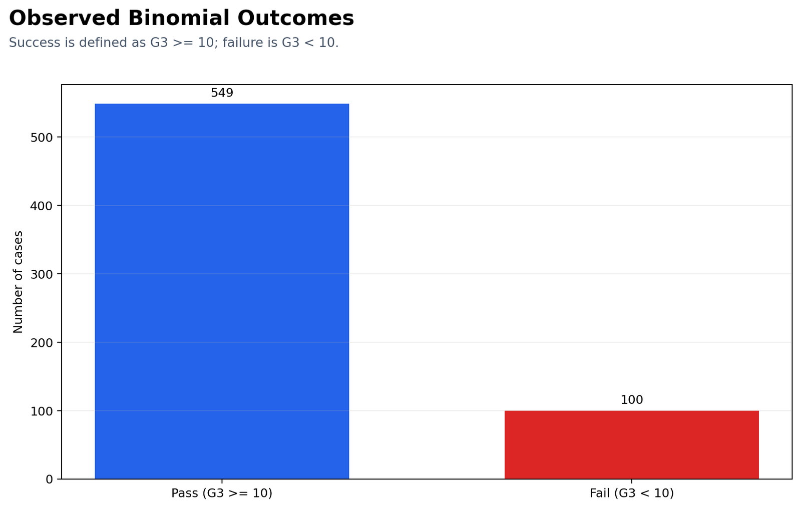
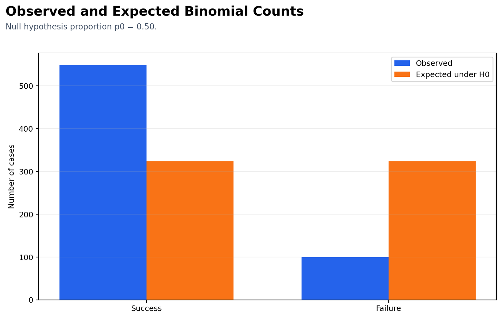
Chart 1: Observed Success and Failure Counts
The count contrast is large: 549 students meet the threshold and 100 do not. The bar heights represent raw frequency, so the success bar is approximately 5.49 times the failure bar. This figure establishes the sample information used by every later Binomial Test calculation.
Chart 2: Observed Versus Expected Counts
Under p0 = .50, both categories have an expected count of 324.5. The observed success count is 224.5 above expectation, and the failure count is 224.5 below expectation. The symmetric deviations explain the extremely small p-value.
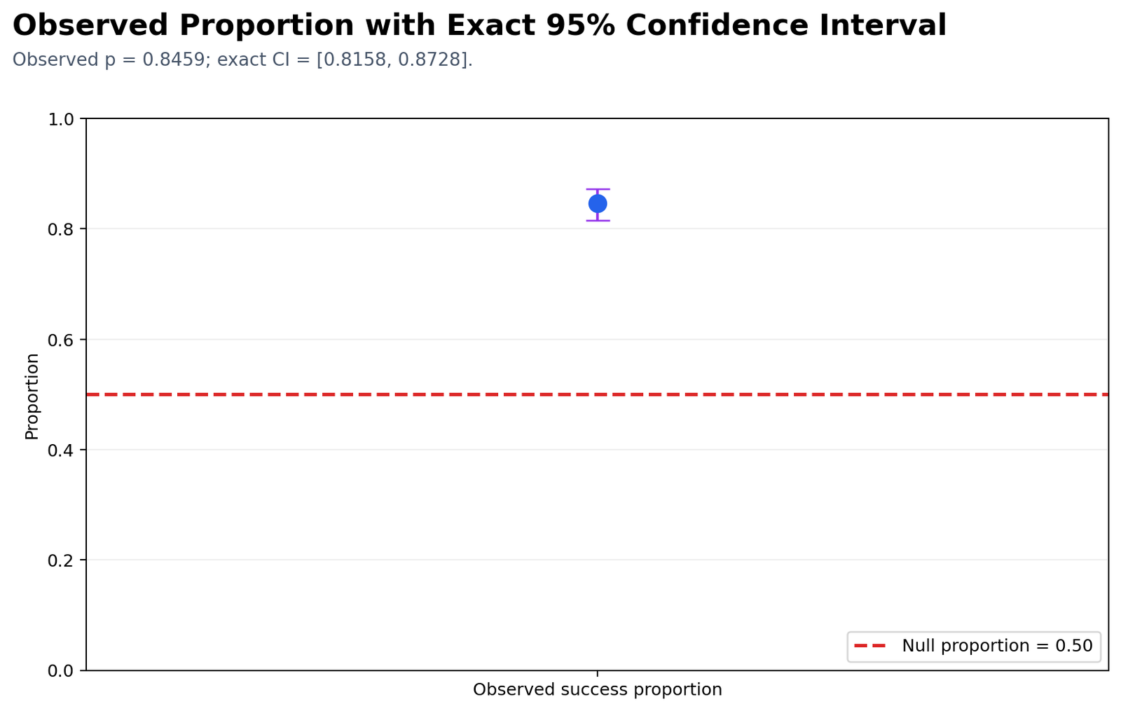
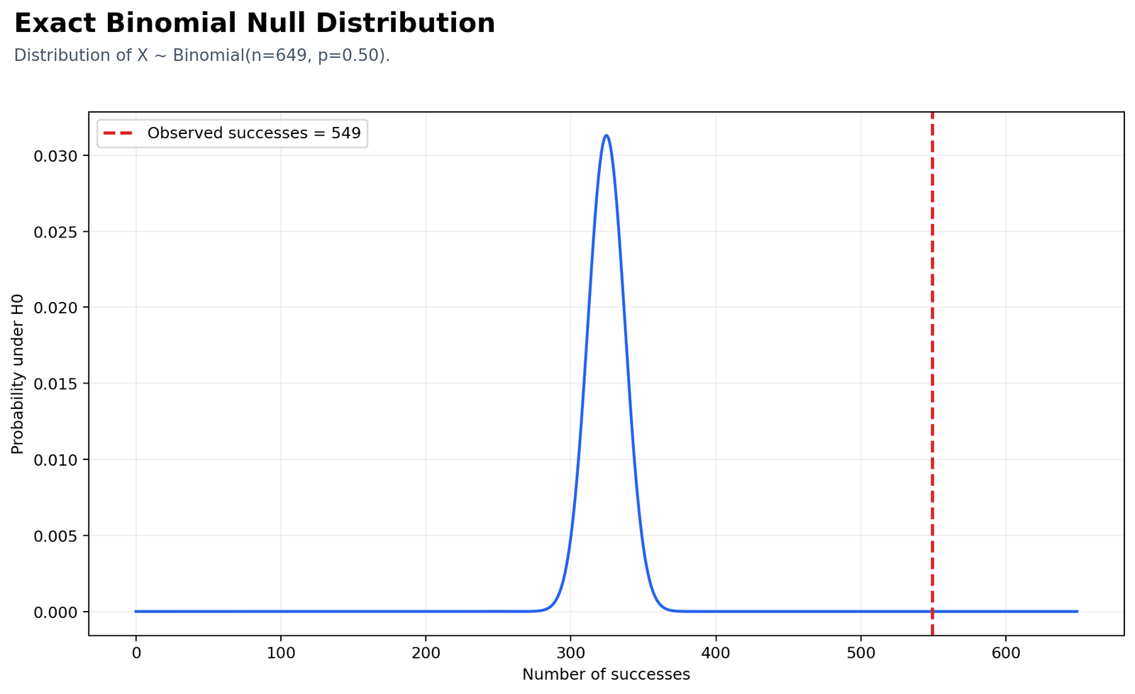
Chart 3: Observed Proportion with Exact 95% CI
The point estimate is 0.8459. The exact interval from 0.8158 to 0.8728 lies entirely above the null line at .50. The chart therefore displays both the estimated magnitude and the uncertainty supporting rejection.
Chart 4: Exact Binomial Null Distribution
The distribution is centred at 324.5 with a standard deviation of 12.7377. The observed count 549 sits 17.62 null standard deviations above the mean and is visually separated from the main probability mass.
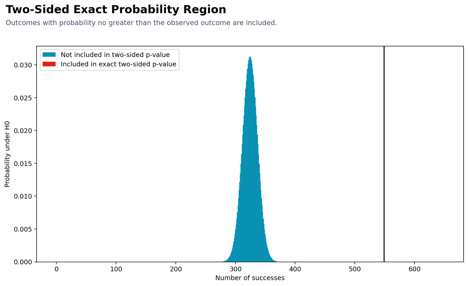
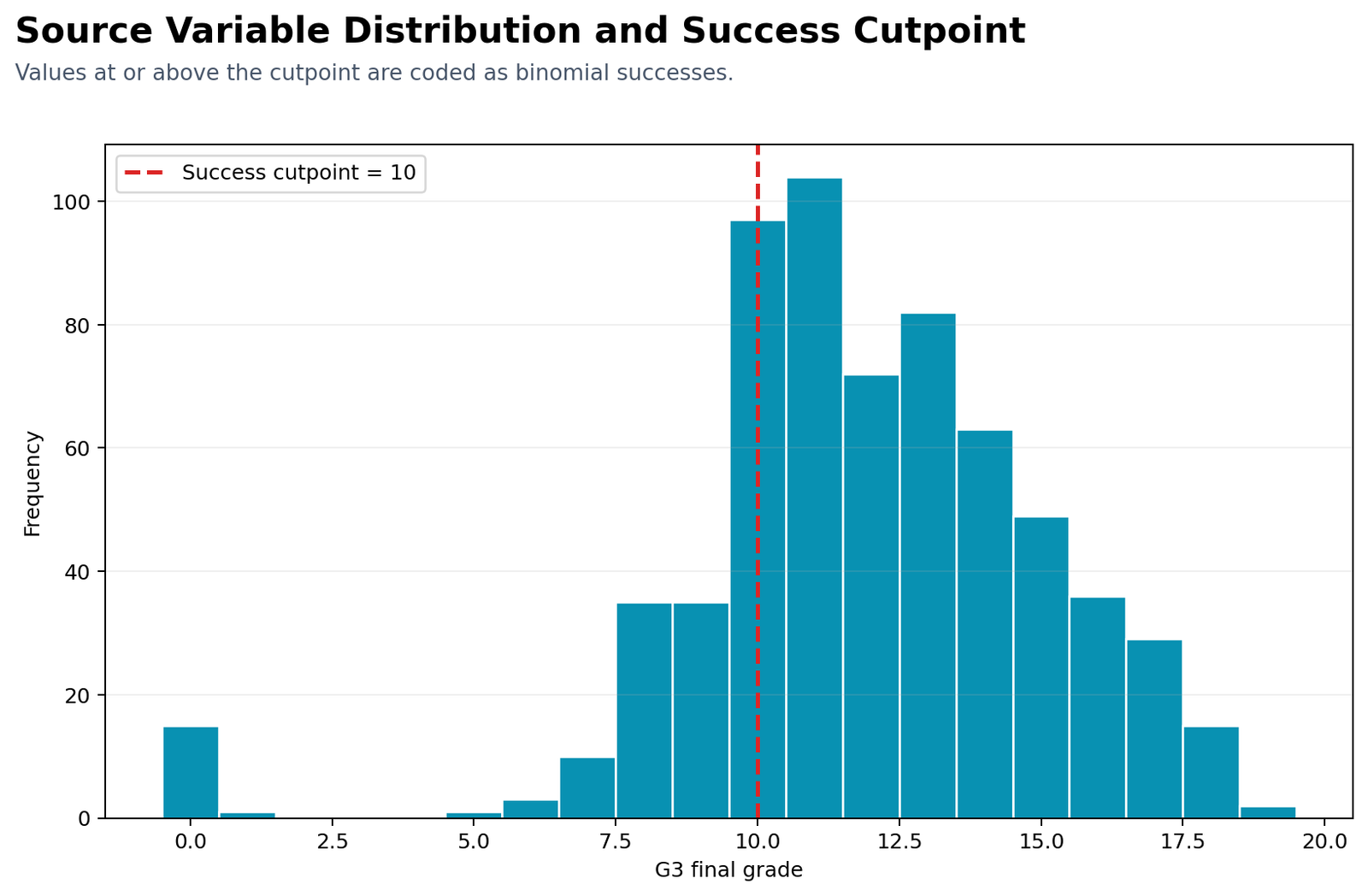
Chart 5: Two-Sided Exact Probability Region
The included outcomes are the far lower and upper probability regions. Because p0 = .50 is symmetric, counts from 0 through 100 match counts from 549 through 649. For an asymmetric null probability, the included two-sided outcomes do not have to be equal-distance tails.
Chart 6: G3 Distribution and Success Cutpoint
The threshold at 10 divides the quantitative grade distribution into 100 values below the cutpoint and 549 at or above it. The most frequent grades are 11, 10, 13, 12 and 14. The chart makes the information loss from dichotomization visible.
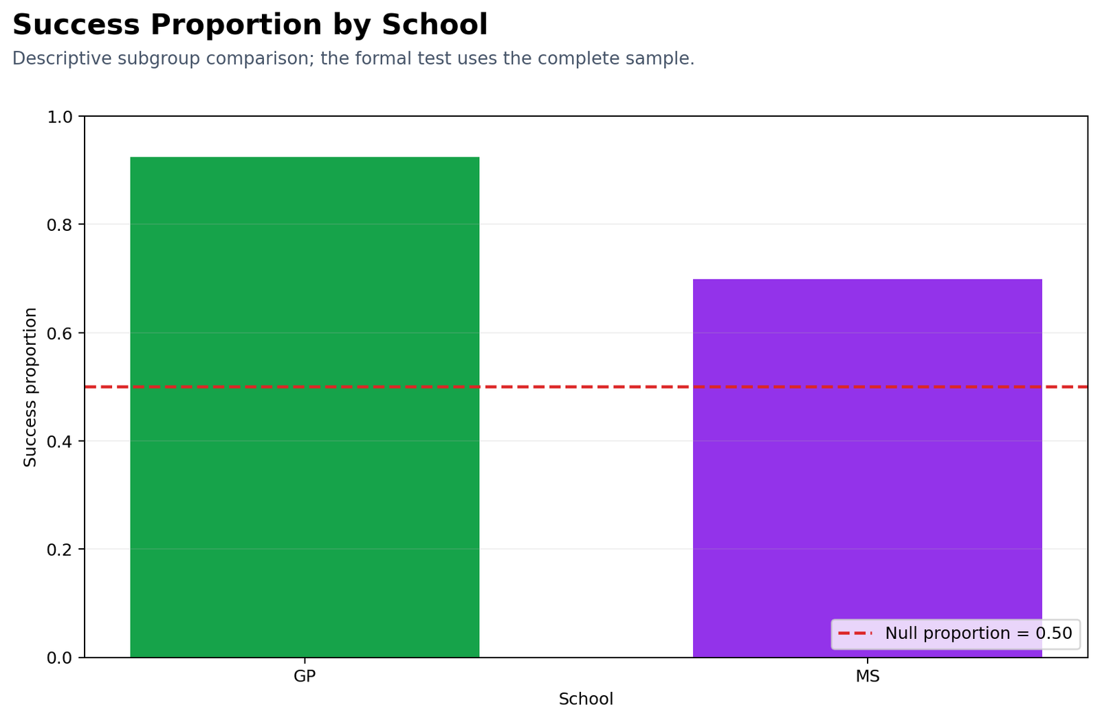
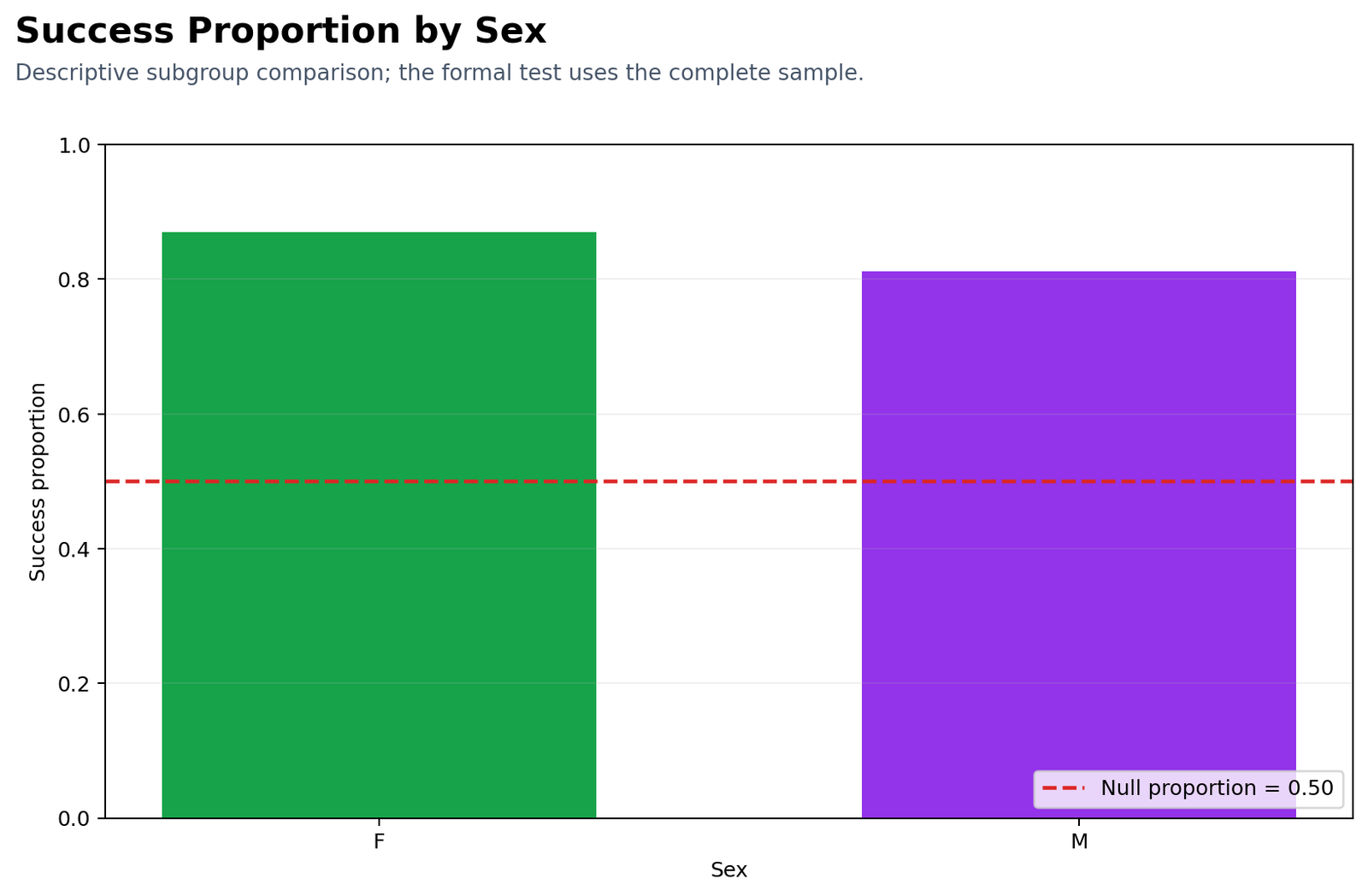
Chart 7: Success Proportion by School
GP has a success proportion of 0.9243, while MS has 0.6991. Both exceed .50, but the school difference is 0.2252, or 22.52%. This is a descriptive subgroup comparison, not the formal one-sample test.
Chart 8: Success Proportion by Sex
Female students have a success proportion of 0.8695, and male students have 0.8120. The difference is 0.0574, or 5.74%. Both subgroup rates remain above the .50 null reference.
Binomial Test in Python, R, SPSS and Excel
Binomial Test in Python
- Use
scipy.stats.binomtest. - Supply k = 549, n = 649, p = 0.50.
- Select
alternative="two-sided". - Request the exact proportion interval from the result object.
- Report p̂, p-value, confidence interval and effect size.
Expected result: p̂ = 0.845917, p = 5.9969e-76, exact 95% CI [0.815805, 0.872838].
Binomial Test in R
- Use
binom.test()from the basestatspackage. - Enter x, n, p, alternative and confidence level.
- R returns the success count, trials, exact p-value and Clopper-Pearson interval.
- The two-sided calculation uses an exact discrete probability rule.
- Use the printed estimate as the observed success proportion.
Expected result: x = 549, n = 649, p-value = 5.9969e-76, estimate = 0.845917.
Binomial Test in SPSS
- Create a numeric binary variable: 1 = G3 ≥ 10, 0 = G3 < 10.
- Use Analyze > Nonparametric Tests > One Sample or the Binomial legacy dialog.
- Set the hypothesized proportion to 0.50.
- Identify 1 as the success category.
- Request a Clopper-Pearson interval when available.
The SPSS hypothesis summary rounds the significance to .000 and rejects H0. Report this as p < .001, not p = .000. The full exact numerical probability is available from Python, R and the worked Excel calculation.
Binomial Test in Excel
- Use
BINOM.DISTfor exact point and cumulative probabilities. - Enumerate all counts from 0 through n for a general two-sided exact p-value.
- Include probabilities no greater than the observed count's probability.
- Use
BETA.INVfor Clopper-Pearson limits. - Use the downloadable workbook for a formula-driven complete analysis.
Important: 2*MIN(lower tail, upper tail) is not a universal replacement for the probability-ordered exact two-sided calculation.
Cross-Software Result Reconciliation
| Software | Primary function or procedure | Worked result | Reporting note |
|---|---|---|---|
| Python | scipy.stats.binomtest | p = 5.9969e-76 | Exact p and exact confidence interval |
| R | binom.test | p = 5.9969e-76 | Exact test with Clopper-Pearson interval |
| SPSS | One-Sample Binomial Test | Sig. displayed as .000 | Write p < .001; verify significance type in the selected procedure |
| Excel | BINOM.DIST + probability-ordering table | p = 5.9969e-76 | Formula-driven reconstruction of all possible counts |
Expandable Binomial Test Code
Python exact Binomial Test and exact confidence interval
from scipy.stats import binomtest
import math

successes = 549
trials = 649
null_proportion = 0.50

result = binomtest(
    k=successes,
    n=trials,
    p=null_proportion,
    alternative="two-sided",
)

exact_ci = result.proportion_ci(
    confidence_level=0.95,
    method="exact",
)

observed_proportion = successes / trials
cohens_h = (
    2 * math.asin(math.sqrt(observed_proportion))
    - 2 * math.asin(math.sqrt(null_proportion))
)

print("Observed proportion:", observed_proportion)
print("Exact p-value:", result.pvalue)
print("Exact 95% CI:", exact_ci.low, exact_ci.high)
print("Cohen's h:", cohens_h)
Python subgroup summaries used in Charts 7 and 8
import pandas as pd
from scipy.stats import binomtest

df = pd.read_csv("dataset.csv")
df["success"] = (df["G3"] >= 10).astype(int)

for variable in ["school", "sex"]:
    summary = (
        df.groupby(variable)["success"]
          .agg(["sum", "count", "mean"])
          .rename(columns={"sum": "successes", "count": "n", "mean": "proportion"})
    )

    intervals = []
    for _, row in summary.iterrows():
        ci = binomtest(
            int(row["successes"]),
            int(row["n"]),
        ).proportion_ci(method="exact")
        intervals.append((ci.low, ci.high))

    summary["exact_ci"] = intervals
    print(variable)
    print(summary)
R exact Binomial Test
successes <- 549
trials <- 649
null_proportion <- 0.50

result <- binom.test(
  x = successes,
  n = trials,
  p = null_proportion,
  alternative = "two.sided",
  conf.level = 0.95
)

print(result)
print(result$estimate)
print(result$conf.int)
print(result$p.value)

observed_proportion <- successes / trials
cohens_h <- 2 * asin(sqrt(observed_proportion)) -
             2 * asin(sqrt(null_proportion))
print(cohens_h)
SPSS one-sample Binomial Test syntax
* Create the binary outcome.
COMPUTE binomial_success = (G3 >= 10).
VALUE LABELS binomial_success
  0 "Failure: G3 below 10"
  1 "Success: G3 at least 10".
EXECUTE.

* Modern one-sample nonparametric workflow.
NPTESTS
  /ONESAMPLE TEST (binomial_success)
    BINOMIAL(
      TESTVALUE=0.50
      SUCCESSCATEGORICAL=LIST(1)
      CLOPPERPEARSON
    )
  /MISSING SCOPE=ANALYSIS USERMISSING=EXCLUDE
  /CRITERIA ALPHA=0.05 CILEVEL=95.

* Legacy Binomial Test; p=.50 gives a two-tailed probability.
NPAR TESTS
  /BINOMIAL(.50)=binomial_success(0,1).
Read the output footnote to determine whether the selected SPSS procedure displays an exact or asymptotic significance value. Never write p = .000.
Excel formulas for the worked Binomial Test
Assume:
B4 = success cutpoint
B5 = null proportion
B6 = alpha
B7 = confidence level

Data sheet:
G2 = --(B2 >= Inputs!$B$4)
Fill G2 downward for all cases.

Summary formulas:
n = COUNT(Data!G2:G650)
x = SUM(Data!G2:G650)
Failures = n-x
Observed proportion = x/n
Expected successes = n*p0
Expected failures = n*(1-p0)
Observed probability = BINOM.DIST(x,n,p0,FALSE)

Exact Clopper-Pearson lower limit:
=IF(x=0,0,BETA.INV(alpha/2,x,n-x+1))

Exact Clopper-Pearson upper limit:
=IF(x=n,1,BETA.INV(1-alpha/2,x+1,n-x))

Cohen's h:
=2*ASIN(SQRT(x/n))-2*ASIN(SQRT(p0))

General exact two-sided p-value:
1. List k = 0,1,...,n.
2. Calculate BINOM.DIST(k,n,p0,FALSE) for each k.
3. Calculate the observed probability at x.
4. Flag each k whose probability is <= observed probability.
5. Sum the flagged probabilities.
Advanced Binomial Testing Topics
Why the exact two-sided p-value is not always twice one tail
The binomial distribution is discrete and can be asymmetric when p0 differs from .50. Doubling the smaller tail can select a different set of outcomes from the probability-ordering rule used by common exact software. State the software or exact definition in reproducible work.
Exact confidence interval and conservatism
The Clopper-Pearson interval is obtained by inverting equal-tailed binomial tests. Its coverage is at least the requested confidence level, which can make it wider than Wilson or likelihood-based intervals. “Exact” does not mean shortest or perfectly centred around p̂.
Does the Binomial Test have a test statistic?
The essential observed information is x and p̂. R labels the success count as the statistic, while SciPy returns the observed proportion as the result statistic. Unlike the one-proportion z-test, the exact calculation does not require a normal-reference z statistic.
Normal approximation for the current sample
Under H0, np0 and n(1−p0) both equal 324.5, so the normal approximation is numerically reasonable. The standardized difference is z ≈ 17.625. The exact Binomial Test is still preferred here because the complete exact probability is readily available.
Power of a Binomial Test
Power depends on n, p0, the true alternative probability, alpha and the alternative direction. Exact power is the sum of alternative-distribution probabilities for counts in the rejection region. See Statistical Power before planning a study.
Sample size for a Binomial Test
Sample-size planning should specify the smallest meaningful difference from p0, target power, alpha and one-sided or two-sided testing. A larger n narrows the confidence interval and allows smaller departures from p0 to be detected.
Multiple Binomial Tests
Running a separate test for many outcomes, subgroups or thresholds increases the familywise false-positive risk. Prespecify the primary outcome and apply a multiplicity strategy when many hypotheses are tested.
Equivalence and noninferiority
Failure to reject p = p0 does not establish that the probability is practically equivalent to p0. Equivalence requires prespecified margins and tests designed to show that the difference is sufficiently small.
Constant probability and observed subgroup differences
The complete-sample Binomial Test treats the sample as one set of trials with one probability. The school proportions 0.924 and 0.699 suggest heterogeneity. If explaining that heterogeneity is the goal, use stratified analysis or logistic regression.
Dichotomization of G3
The threshold analysis discards differences within each side of the cutpoint. A grade of 10 and a grade of 19 both count as success. The binary analysis should be justified by the research question and can be supplemented with analysis of the original G3 scale.
Mid-p Binomial Test
A mid-p procedure subtracts half the probability of the observed count from a conventional exact tail. It can reduce conservatism but does not provide the same exact size guarantee. Label a mid-p result explicitly and do not mix it with the full exact p-value.
Bayesian alternative
A Bayesian one-sample binomial analysis combines a prior distribution with the observed successes and failures to obtain a posterior distribution for p. It answers probability statements about p rather than a frequentist tail-probability question.
Finite population sampling
When a large fraction of a finite population is sampled without replacement, the Bernoulli trials are dependent. A hypergeometric model or finite-population correction may be more appropriate than the ordinary Binomial Test.
APA Reporting for the Binomial Test
The APA reporting section should state the success definition, number of successes, total sample size, observed proportion, null proportion, alternative, exact p-value, exact confidence interval and substantive interpretation. The exact p-value is extremely small in this example, so the main prose uses p < .001 while the technical table retains the scientific-notation value.
Full APA-Style Result for the Worked Example
An exact two-sided Binomial Test showed that the proportion of students with G3 ≥ 10 (549/649, p̂ = 0.846) was significantly different from the hypothesized proportion of 0.50, p < .001, exact 95% CI [0.816, 0.873]. The observed proportion was 34.59% above the null value, and Cohen's h was 0.764, indicating a substantial standardized difference.
Concise APA-Style Result
The G3 ≥ 10 proportion was 0.846 (549/649), which differed from .50, exact p < .001, 95% CI [0.816, 0.873].
APA-Style Methods Sentence
A two-sided exact Binomial Test was used to compare the observed proportion of students with G3 ≥ 10 with a hypothesized population proportion of .50. Exact Clopper-Pearson confidence limits were calculated at the 95% level.
APA-Style Results Table
| Measure | Value | APA presentation |
|---|---|---|
| Success definition | G3 ≥ 10 | State in text or table note |
| Successes / total | 549 / 649 | 549/649 |
| Observed proportion | 0.845916795 | .846 |
| Null proportion | 0.50 | .50 |
| Exact p-value | 5.9969047562e-76 | < .001 in prose |
| Exact 95% CI | [0.815805378, 0.872838333] | [.816, .873] |
| Cohen's h | 0.764025 | .764 |
Reusable APA Templates for the Binomial Test
Significant Two-Sided Binomial Test
An exact two-sided Binomial Test evaluated whether the outcome proportion differed from p0. The outcome occurred in x of n observations (p̂ = observed proportion).
The observed proportion differed significantly from the null proportion, exact p = p-value.
The exact 95% confidence interval was [lower, upper], and the effect size was Cohen's h = h.
Use the exact numerical p-value when it is readable; use p < .001 when the value is extremely small.
Nonsignificant Two-Sided Binomial Test
An exact two-sided Binomial Test compared the observed outcome proportion (x/n, p̂ = proportion) with p0.
The result was not statistically significant, exact p = p-value.
The analysis did not provide sufficient evidence that the population proportion differed from p0; it did not prove that the two values were identical.
Always include the confidence interval so readers can see which population proportions remain plausible.
Prespecified Directional Binomial Test
A one-sided exact Binomial Test evaluated the prespecified hypothesis that the outcome probability was greater than / less than p0.
The result was statistically significant / not statistically significant, exact p = p-value.
The observed proportion was proportion, based on x successes in n trials.
Use directional wording only when the alternative was selected before examining the data.
APA Rounding and Language
| Avoid | Use instead | Reason |
|---|---|---|
| p = .000 | p < .001 | The probability is extremely small, not zero. |
| The Binomial Test proved p ≠ .50 | The test provided evidence that p differed from .50 | Hypothesis tests do not prove a population statement. |
| The result was important because it was significant | The result was significant and the observed difference was 34.59 percentage points | Magnitude and significance are separate. |
| The null was accepted | The null was not rejected | Nonsignificance does not establish equality. |
| The success rate was 0.846% | The success rate was 84.6% | Proportion-to-percentage conversion must multiply by 100. |
Common Binomial Test Mistakes and How to Correct Them
| Common mistake | Why it is wrong | Correct approach |
|---|---|---|
| Calling the method a binomial t test | A t-test evaluates means, not one binary probability. | Use “Binomial Test” or “exact Binomial Test.” |
| Using the test to compare two groups | A one-sample Binomial Test compares one p with a fixed p0. | Use a two-proportion or exact 2 × 2 method. |
| Doubling the smaller tail automatically | This can disagree with probability-ordering for asymmetric discrete distributions. | Use the exact definition implemented by the selected software. |
| Reporting p = .000 | The probability is not exactly zero. | Report p < .001 or the scientific-notation value. |
| Ignoring the success definition | Readers cannot reproduce x or interpret direction. | State the event category and cutpoint. |
| Assuming exact means assumption-free | The binomial model still requires binary, independent, constant-probability trials. | Assess the design assumptions directly. |
| Selecting one-sided after seeing the result | This inflates false-positive risk. | Prespecify the alternative. |
| Using separate subgroup bars as a group-comparison test | Descriptive proportions do not test equality between groups. | Use a direct two-group method. |
| Reporting only the p-value | Magnitude and uncertainty are missing. | Report p̂, exact CI and an effect measure. |
| Ignoring dichotomization | The binary threshold discards information in G3. | Justify the cutpoint and consider a full-scale analysis. |
| Using a normal approximation with tiny expected counts | The z reference can be inaccurate. | Use the exact Binomial Test. |
| Interpreting nonsignificance as equality | Failure to reject is not proof of no difference. | Interpret the interval and consider equivalence methods. |
Binomial Test Reports and Worked Excel Download
R Binomial Test ReportExact binom.test output, interpretation and eight chart pages.
SPSS Binomial Test OutputBinary frequencies, hypothesis summary, G3 distribution and subgroup crosstabs.
Worked Binomial Test Excel WorkbookFormula-driven data, exact null distribution, confidence interval, reporting and editable inputs.
Frequently Asked Questions About the Binomial Test
The Binomial Test questions below address assumptions, formula, calculator use, exact probability, software, interpretation and APA reporting without repeating the full worked sections above.
What is a Binomial Test?
A Binomial Test is an exact one-sample test of whether a binary outcome probability equals a specified value.
What are the Binomial Test hypotheses?
The null is p = p0. The alternative can be p ≠ p0, p > p0 or p < p0.
When should a Binomial Test be used?
Use it for one sample of binary, independent, constant-probability observations with a fixed n and a prespecified null probability.
What are the Binomial Test assumptions?
The outcome is binary, trials are independent, n is fixed, the success probability is constant and the null probability is specified.
Is the Binomial Test only for small samples?
No. It is exact for any sample size under the binomial model. Approximate methods become more accurate as n grows.
What is the exact Binomial Test formula?
It uses P(X=k)=C(n,k)p0^k(1-p0)^(n-k) and sums the probabilities in the selected exact tail region.
How is a two-sided exact p-value calculated?
Common software sums probabilities of outcomes no more probable than the observed outcome under H0.
Can I always double a one-sided p-value?
No. That shortcut can disagree with probability-ordering when the null binomial distribution is asymmetric.
What is a one tailed Binomial Test?
It tests whether p is specifically greater than or less than p0 and should be selected before viewing the result.
What is a two tailed Binomial Test?
It tests whether p differs from p0 in either direction.
What is the observed proportion in this example?
The observed proportion is 549/649 = 0.845917, or 84.59%.
What is the exact p-value in this example?
The exact two-sided p-value is approximately 5.9969e-76.
What is the exact confidence interval?
The Clopper-Pearson 95% interval is [0.815805, 0.872838].
What does Cohen's h mean?
Cohen's h standardizes the difference between p-hat and p0. Here h = 0.764, close to the conventional large benchmark.
Does the Binomial Test have a test statistic?
R reports the success count, while SciPy reports the observed proportion. The exact test does not need a normal-reference z statistic.
What is a binomial t test?
It is usually a mistaken phrase. Use a t-test for a quantitative mean and a Binomial Test for a binary probability.
Is a Binomial Test nonparametric?
Software may place it among nonparametric tests, but it still assumes a specific binomial probability model.
Can a Binomial Test compare two groups?
Not directly. Use a two-proportion test or a suitable exact 2 x 2 method.
Can a Binomial Test adjust for covariates?
No. Use binary logistic regression when predictors or adjustment variables are required.
How do I run a Binomial Test in Python?
Use scipy.stats.binomtest with k, n, p and an alternative.
How do I run a Binomial Test in R?
Use binom.test(x, n, p, alternative, conf.level).
How do I run a Binomial Test in SPSS?
Create or select a dichotomous variable, set the test proportion and identify the success category in the one-sample nonparametric procedure.
How do I run a Binomial Test in Excel?
Use BINOM.DIST for each possible count, sum probability-ordered outcomes and use BETA.INV for exact confidence limits.
Why does SPSS display .000?
SPSS rounds very small significance values. Report p < .001 rather than p = .000.
What is the difference between exact and approximate tests?
The exact test uses the finite binomial distribution; an approximate z-test uses a normal reference.
Does the Binomial Test require normality?
No. The binary count follows a binomial model, not a normal outcome distribution.
Why is the school chart descriptive?
The formal test uses the complete sample. Comparing school proportions directly requires a two-group test.
Why can subgroup probabilities differ?
The simple one-sample model averages across subgroup heterogeneity. Different predictors may be related to the outcome.
What is the success cutpoint in this example?
Success is defined as G3 at least 10.
How should the result be reported in APA style?
Report 549/649, p-hat = .846, p0 = .50, exact p < .001, exact 95% CI [.816, .873] and Cohen's h = .764.
What is the main conclusion?
The observed success rate of 84.59% is substantially higher than the hypothesized 50% rate.
Binomial Test Conclusion
The Binomial Test is an exact one-sample method for evaluating a binary population proportion. It is appropriate when the outcome is binary, the trials are independent, the number of trials is fixed and the probability is constant under the simple model.
In the worked example, 549 of 649 students had G3 ≥ 10, giving an observed proportion of 0.845917. The exact two-sided p-value was 5.9969e-76, and the exact 95% confidence interval was [0.8158, 0.8728]. The null proportion of .50 was rejected.
The difference was also substantial in magnitude: the observed proportion was 34.59% above the null, and Cohen's h was 0.764. The final report should include the success definition, x, n, p̂, p0, exact p-value, exact confidence interval and effect size.

