
Simple Linear Regression: Formula, Slope, R-Squared, Prediction, Python, R, SPSS and Excel
Simple Linear Regression estimates a straight-line relationship between one predictor and one continuous outcome. This complete worked guide predicts final grade G3 from second-period grade G2 for 649 student records, verifies the equation, correlation, ANOVA, confidence and prediction bands, residuals, influence diagnostics and Python, R, SPSS and Excel evidence.
Simple Linear Regression Model Overview
Simple Linear Regression is the ordinary least-squares model used when one continuous predictor is expected to explain or predict one continuous outcome through a straight-line conditional mean. The model answers a focused question: how much does the expected outcome change when the predictor increases by one unit?
In the worked analysis, G3 is the final-grade outcome and G2 is the second-period-grade predictor. The model uses 649 complete records and estimates the equation G3̂ = 0.121966 + 1.018490(G2). The slope is interpreted in original grade points, making the result immediately understandable to a new student.
Simple Linear Regression differs from correlation because the model explicitly names an outcome and supplies a prediction equation. Pearson correlation remains symmetric and unit-free. It differs from Multiple Linear Regression because no additional predictors are controlled. The simple slope therefore summarizes the total sample association between G2 and G3 rather than the conditional effect of G2 after adjustment.
Ordinary least squares chooses the intercept and slope that minimize the sum of squared vertical residuals. The method gives large residuals disproportionate influence because every residual is squared. This fitting rule creates exact algebraic properties: residuals sum to zero, the line passes through the sample means, and the overall F test equals the squared slope t test when only one predictor is included.
A Simple Linear Regression coefficient is interpreted on the outcome scale. The fitted G2 coefficient of 1.018490 means that a one-point increase in G2 is associated with an estimated 1.018490-point increase in expected G3. This is an association under the one-predictor model, not proof that changing G2 would causally change G3 by that amount.
The method supports a continuous outcome and a numeric predictor, or a binary predictor coded numerically when a two-group mean comparison is intended. Its central assumptions remain a meaningful straight-line conditional mean, independent observations, suitable residual variance treatment and no small set of cases dominating the equation. Normal residuals are most important for exact small-sample t and F inference; they are not required merely to calculate the fitted line.
The advantages are transparency, direct hand calculation, clear slope units and a close connection among correlation, R² and ANOVA. The limitations are omitted-variable vulnerability, an unbounded fitted line for a bounded grade outcome, sensitivity to large residuals and the danger of confusing strong prediction with causation.
The worked evidence is unusually strong in the central relationship: Pearson r = 0.918548, R² = 0.843730 and slope t = 59.103989. At the same time, the residual distribution contains a severe negative tail, with skewness −2.941425 and kurtosis 21.789655. The correct conclusion must therefore combine strong average fit with transparent individual-level diagnostic limitations.
Quick Answer
The verified Simple Linear Regression evidence supports a strong positive line and a nearly one-for-one grade relationship.
Stable Simple Linear Regression evidence
- G2 slope = 1.018490.
- 95% slope CI = [0.984653, 1.052328].
- F(1,647) = 3493.281566.
- Python, R, SPSS and Excel reproduce the core equation.
Important diagnostic limits
- Residual skewness = −2.941425.
- Residual kurtosis = 21.789655.
- Maximum |studentized residual| = 7.602273.
- Maximum Cook’s distance = 0.086831.
Table of Contents
- Model Overview
- Quick Answer
- Why Simple Linear Regression Is Needed
- How Simple Linear Regression Works
- Variables and Coding
- Verified Results
- Python Chart Stories
- R Chart Pairs
- Coefficient Interpretation
- Predictions and Meaning
- Assumptions and Diagnostics
- Python, R, SPSS and Excel
- Code and Formulas
- Advanced Topics
- APA-Style Reporting
- Publication Checklist
- Downloads
- Related Guides
- Frequently Asked Questions
- Conclusion
Why This Analysis Needs Simple Linear Regression
The research question contains one continuous predictor, G2, and one continuous outcome, G3. The scatterplot shows a strong positive pattern, and the purpose is to quantify that pattern with one slope, one intercept, explained variance and prediction uncertainty.
A simple model is valuable before richer adjustment because it provides a transparent benchmark. It shows how much predictive information G2 contains by itself and supplies exact values against which Multiple Linear Regression, Polynomial Regression or robust alternatives can be compared.
The method does not need additional predictors to answer the unadjusted prediction question. Adding variables would change the estimand from the total sample relationship to a conditional one. That richer question may be useful, but it is not identical to the Simple Linear Regression question answered here.
How Simple Linear Regression Works
Least-Squares Objective
The residual for each student is observed G3 minus fitted G3. Squared residuals are summed, and the equation with the smallest total is selected.
Slope and Intercept
The intercept anchors the line through the sample means. The slope converts one predictor point into expected outcome points.
Four-Step Calculation Flow
Worked Prediction
If the observed G3 is 11, the residual is −0.325360. The negative sign means the observed outcome is below the fitted average.
Variables Used, Coding and Standardization
The analysis uses the original grade-point units. No automatic standardization is applied to the primary equation, so the slope remains directly interpretable.
| Role | Variable | Definition | Coding or unit | Simple Linear Regression use |
|---|---|---|---|---|
| Outcome | G3 | Final grade | Continuous grade; observed range 0–19 | Predicted conditional mean |
| Predictor | G2 | Second-period grade | Continuous grade; observed range 0–19 | One-point slope interpretation |
| Model output | Fitted G3 | Predicted average final grade | Continuous | 0.121966 + 1.018490×G2 |
| Diagnostic output | Residual | Observed G3 minus fitted G3 | Continuous error | Positive above line; negative below line |
| Uncertainty | Mean confidence band | Average G3 at one G2 value | 95% interval | Narrower near mean G2 |
| Uncertainty | Prediction interval | One future G3 at one G2 value | 95% interval | Includes residual outcome variation |
The same 649 complete rows and intercept convention are used in every software implementation. Changing missing-data handling or removing the intercept would change the equation and invalidate a direct comparison.
Verified Simple Linear Regression Results
Model Performance
| Metric | Exact value | Interpretation |
|---|---|---|
| Observations | 649 | All complete G2–G3 pairs |
| Pearson correlation | 0.918548 | Strong positive linear association |
| R² | 0.843730 | 84.373% of fitted-sample G3 variance explained |
| Adjusted R² | 0.843489 | Nearly identical because one predictor is used |
| RMSE | 1.276125 | Squared-error prediction summary in G3 points |
| MAE | 0.808023 | Average absolute fitted error |
| Residual standard error | 1.278096 | Conditional noise estimate using 647 df |
| AIC | 2144.9520 | Information criterion for this fitted Gaussian model |
| BIC | 2158.3823 | Information criterion with stronger complexity penalty |
The difference between RMSE and residual standard error is expected because the denominators differ. The residual standard error uses 647 residual degrees of freedom, whereas the reported RMSE uses the number of observations.
Regression ANOVA
| Source | Sum of squares | df | Mean square | F | p-value |
|---|---|---|---|---|---|
| Regression | 5706.373839 | 1 | 5706.373839 | 3493.281566 | 5.6424 × 10−263 |
| Residual | 1056.892725 | 647 | 1.633528 | — | — |
| Total | 6763.266564 | 648 | — | — | — |
The overall F statistic tests whether the one-predictor model improves on an intercept-only mean model. Because only one slope is tested, F equals the squared slope t statistic.
Coefficient Estimates
| Term | B | SE | t | p | 95% CI | Simple Linear Regression reading |
|---|---|---|---|---|---|---|
| Intercept | 0.121966 | 0.205593 | 0.593240 | .553228 | [−0.281745, 0.525677] | Baseline at G2 = 0 is imprecise |
| G2 | 1.018490 | 0.017232 | 59.103989 | 5.6424 × 10−263 | [0.984653, 1.052328] | Strong positive grade-point slope |
G2 provides the substantive result. Its interval is narrow, positive and centered near one. The intercept is retained because the fitted model requires a baseline and because removing it would change the slope, R² and residual structure.
Download the Simple Linear Regression Reports
The same report links appear again in the Downloads section.
Python Charts and Exact-Value Explanations
The five verified Python assets are explained with the attached format’s pattern, key values, interpretation and practical reason each figure matters.
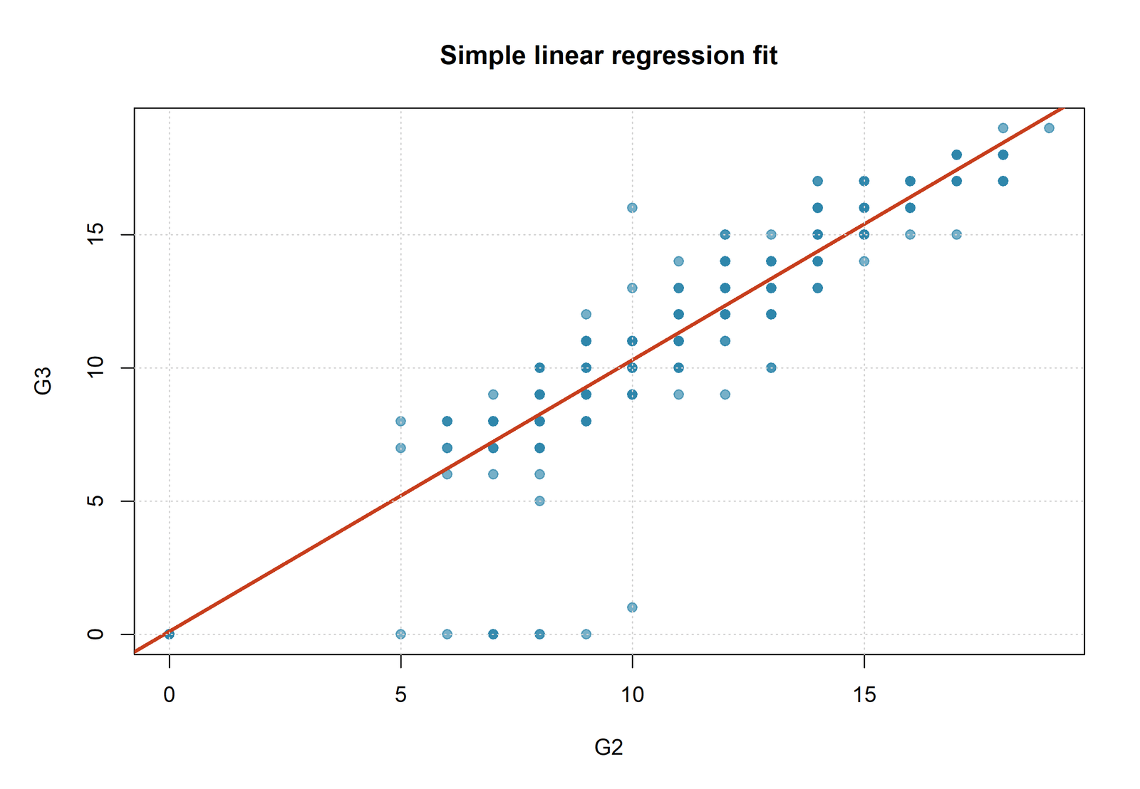
Python Chart 1: G2–G3 Scatterplot and Fitted Line
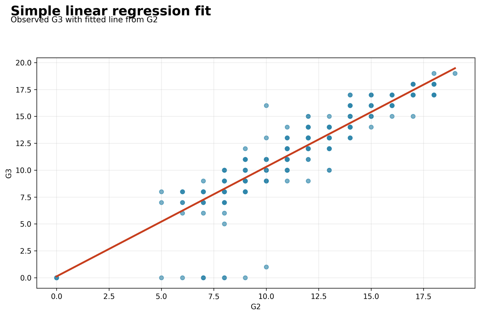
The points form a dense upward diagonal band. A smaller group of zero final grades lies far below the main pattern even when G2 is in the ordinary range.
The fitted equation is G3̂ = 0.121966 + 1.018490(G2). Pearson r = 0.918548 and R² = 0.843730.
Expected G3 increases almost one point for each additional G2 point. The zero-grade cases do not erase the central positive relationship, but they create the largest negative residuals.
The chart establishes the mean structure and reveals why Outlier Detection and residual review remain necessary.
Python Chart 2: Mean Confidence Band around the Fitted Line
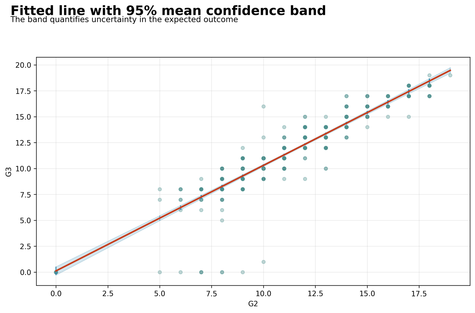
The band is narrowest around mean G2 and widens toward the predictor edges. The fitted line remains the center of the band at every G2 value.
At G2 = 11, predicted G3 is 11.325360 and the 95% mean-response interval is approximately [11.224974, 11.425746].
The band estimates the population mean G3 for a given G2. It does not describe the likely range for one individual student.
The distinction is essential when reporting a Confidence Interval rather than a prediction interval.
Python Chart 3: Residuals versus Predicted Values
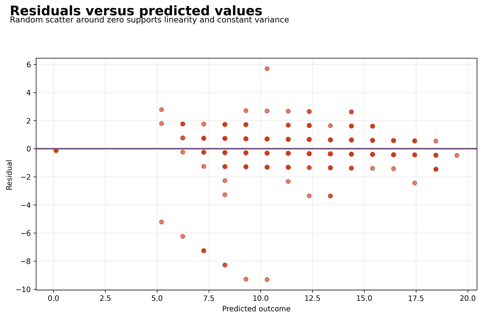
Residual bands arise because G3 is recorded in integer grade points. Several observations extend sharply downward from the main cloud.
RMSE = 1.276125, MAE = 0.808023 and residual standard error = 1.278096.
Most errors are modest, but a small number of extreme negative errors dominate tail diagnostics. Strong overall fit therefore coexists with important individual misses.
Inspect Studentized Residuals, Cook’s Distance and Influence Diagnostics.
Python Chart 4: Residual Normal Q-Q Plot
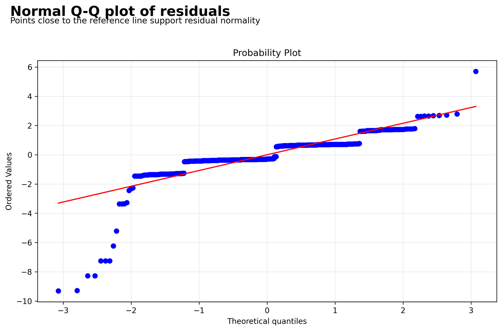
The central residuals are much closer to the reference line than the lower tail. The most negative errors bend dramatically away from normal-theory expectations.
Shapiro–Wilk W = 0.710847, p = 6.0596 × 10⁻³², skewness = −2.941425 and kurtosis = 21.789655.
Exact normal-error assumptions are not supported. The large sample helps slope estimation, but conventional prediction and tail inference still deserve sensitivity analysis.
Use the Q-Q Plot Normality Check, Shapiro-Wilk Test and Skewness and Kurtosis guides.
Python Chart 5: Observed versus Predicted G3
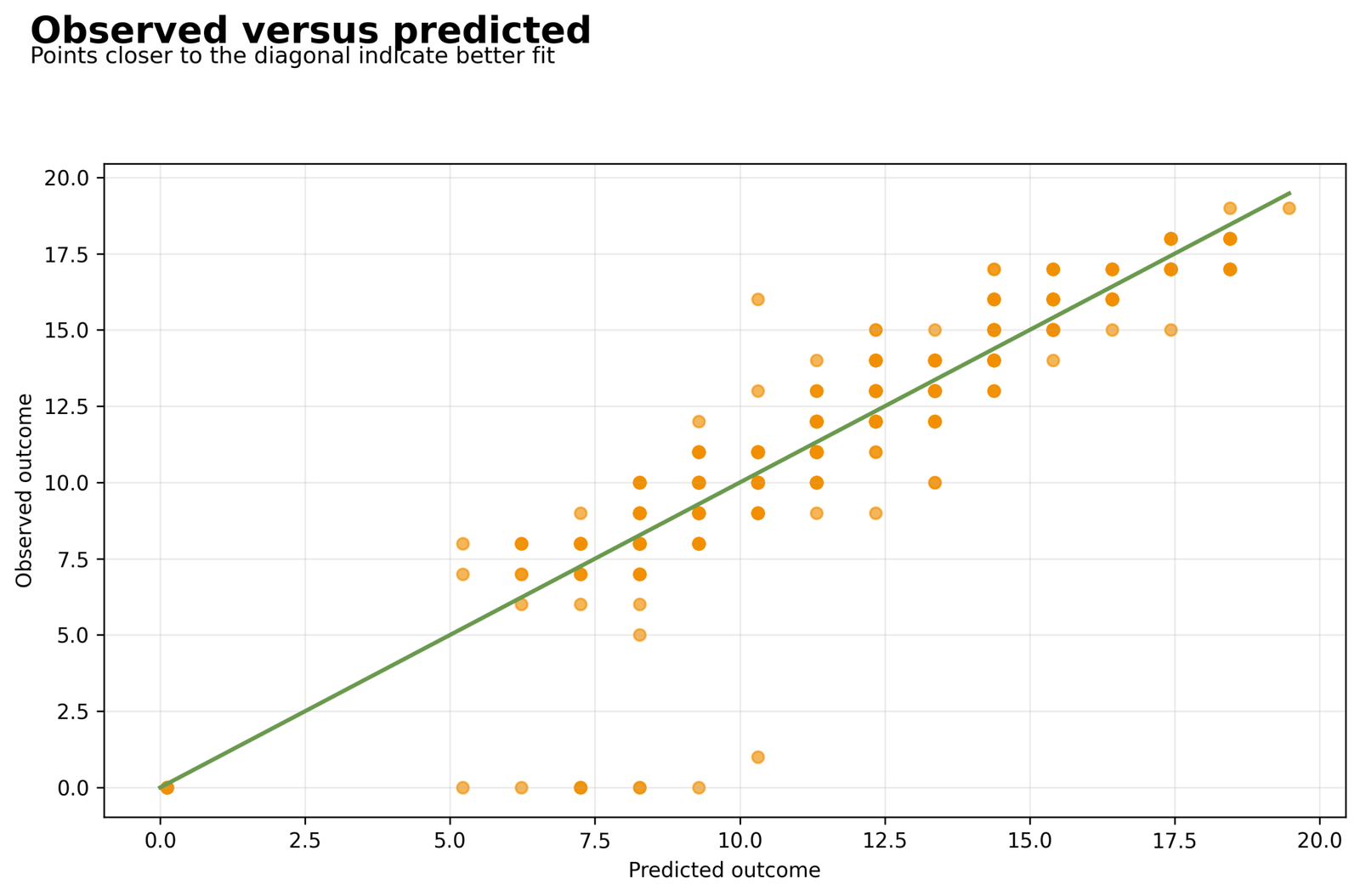
Most points follow the diagonal in the central grade range. Horizontal bands reflect integer observed grades, while several zero outcomes fall far below the diagonal.
R² = 0.843730, adjusted R² = 0.843489 and F(1,647) = 3493.281566.
The model reproduces overall grade ordering very well, but individual prediction is weaker for the extreme low-outcome cases.
Report Adjusted R-Squared with error metrics rather than describing R² as the percentage of students predicted correctly.
R Charts and Paired Explanations
The R evidence independently cross-checks the Simple Linear Regression calculations. Four unique R assets are arranged in two matched pairs with a dedicated explanation beneath each chart.
R Chart 1: Mean Confidence and Individual Prediction Bands
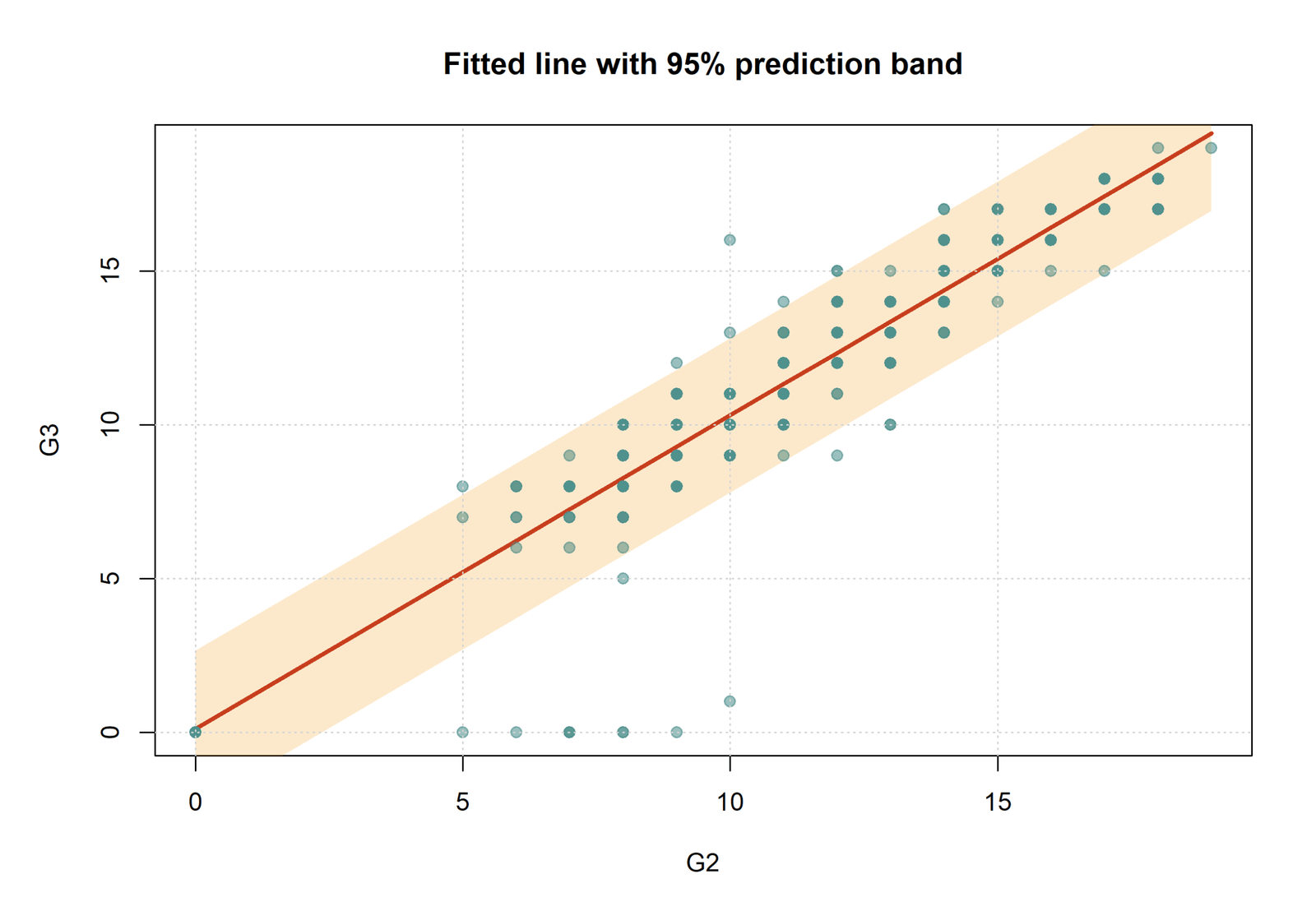
Pattern: The narrow band estimates the average response and the wider band estimates one future outcome. Both are centered on the same fitted line.
Key values: At G2 = 11, the mean interval is approximately [11.2250, 11.4257], while the individual prediction interval is approximately [8.8136, 13.8371].
Interpretation: Individual prediction uncertainty is much larger because residual variation is added to line-estimation uncertainty.
R Chart 2: Residual Distribution
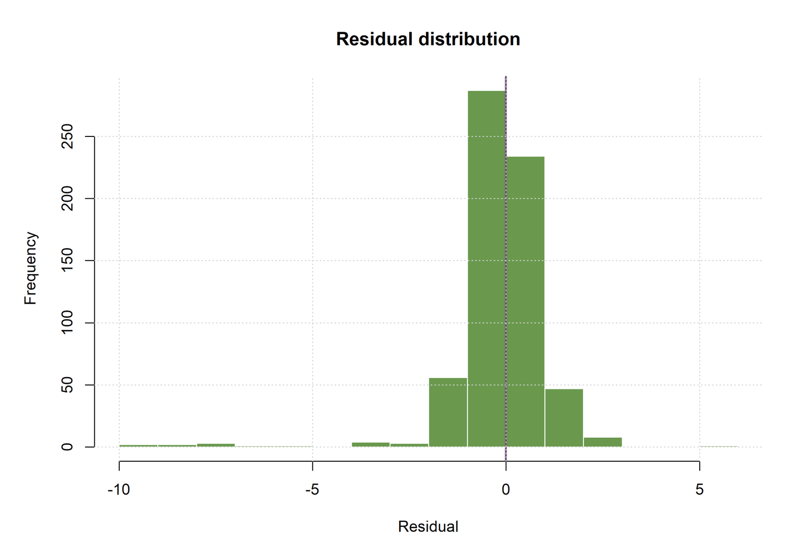
Pattern: The central residual mass is concentrated near zero, but the lower tail is much longer than the upper tail.
Key values: Residual skewness is −2.9414, kurtosis is 21.7897 and the Shapiro–Wilk p-value is 6.06 × 10⁻³².
Interpretation: The histogram confirms that a few extremely negative errors drive the non-normal tail rather than a broad failure of the central fitted relationship.
R Chart 3: Leverage, Studentized Residuals and Cook’s Distance
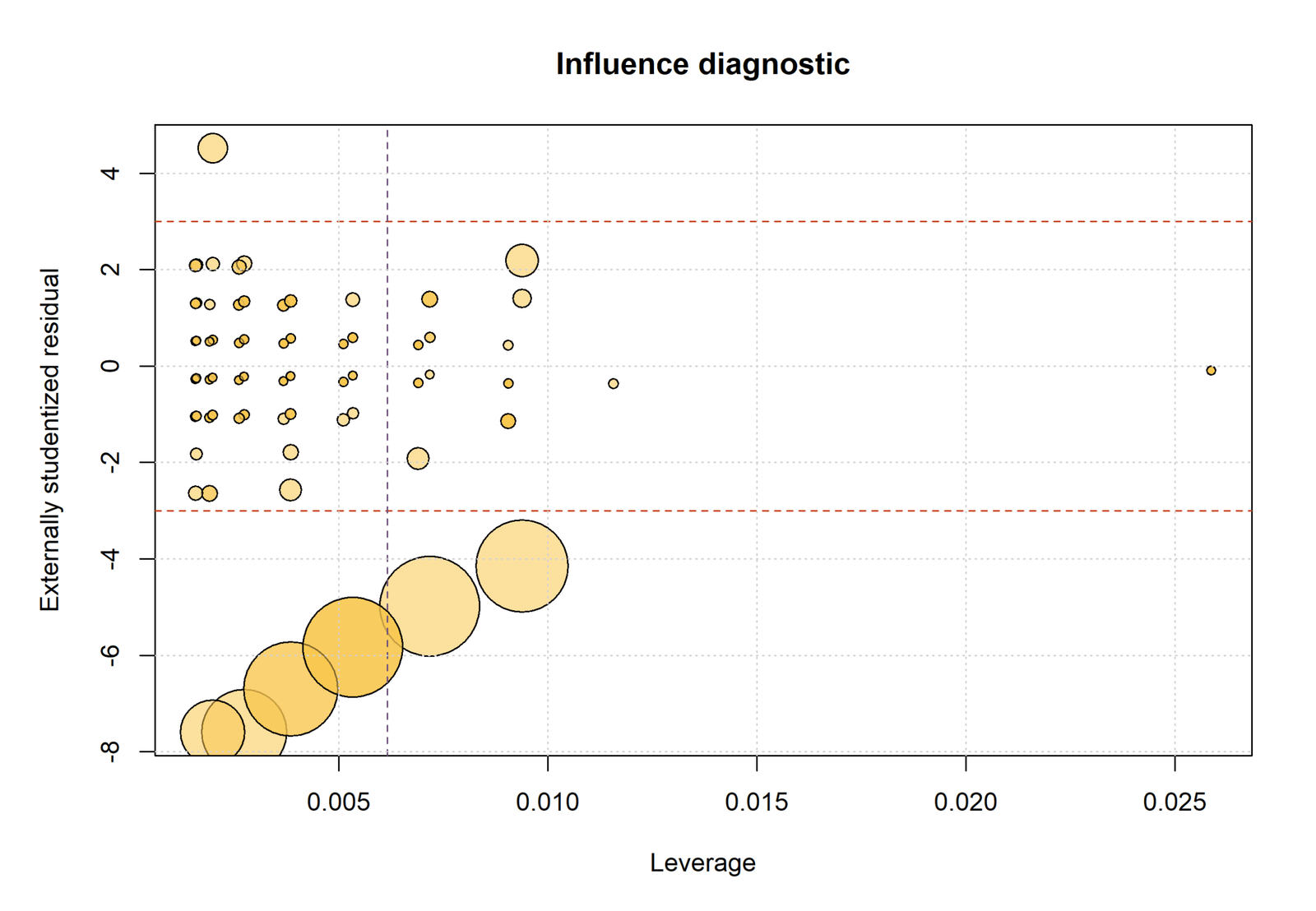
Pattern: Most observations have low leverage and modest residuals. A smaller group combines large vertical errors with enough leverage to affect the fitted line.
Key values: Maximum |studentized residual| = 7.602273, maximum leverage = 0.025876 and maximum Cook’s distance = 0.086831.
Interpretation: Influence is not the same as being unusual on G3 alone. It reflects residual size, predictor position and their effect on the estimated equation.
R Chart 4: Independent Fitted-Line Verification
Pattern: The R plot reproduces the same positive line and the same difficult zero-grade observations visible in Python.
Key values: R and Python agree on intercept 0.121966, slope 1.018490, Pearson r 0.918548 and R² 0.843730.
Interpretation: Cross-software agreement confirms the core calculation when rows, formula and intercept convention are identical.
Simple Linear Regression Coefficient and Parameter Interpretation
Primary Equation
The G2 coefficient is the expected G3 difference associated with a one-point G2 difference. Holding nothing else constant because no other predictor is included, a student one point higher on G2 has approximately 1.0185 points higher fitted G3.
The slope confidence interval [0.984653, 1.052328] indicates that every plausible value under the classical model is positive and close to one grade point. Statistical precision is high because the sample is large, G2 varies substantially and the G2–G3 association is strong.
The intercept of 0.121966 is the fitted G3 at G2 = 0. Its p-value is .553228. The intercept is not the main research target, and its nonsignificance does not justify a no-intercept model.
Pearson r = 0.918548 and R² = 0.843730 describe association strength and explained sample variation. Neither statistic measures causal effect, individual prediction certainty or the proportion of students predicted exactly.
Predictions, Effects and Model Meaning
A Simple Linear Regression prediction is obtained by substituting a G2 value into the fitted equation. At G2 = 11, the fitted mean G3 is 11.325360.
The mean-response interval is narrow because it estimates the average outcome for a predictor value. The individual interval is much wider because it includes person-to-person residual variation around that average.
The prediction is not automatically constrained to the grade scale. The fitted equation should therefore be used within the observed G2 range and interpreted cautiously near boundaries.
Simple Linear Regression Assumptions and Diagnostics
The expected G3 relationship should be reasonably straight across G2.
Students should be independent at the modeled sampling level.
No few observations should determine the slope and intercept.
Linearity
The scatterplot shows a strong straight-line pattern, but residual plots should still be inspected for curvature. Use Ramsey RESET Test and compare with Polynomial Regression if a systematic bend remains.
Residual Variance
Use Breusch-Pagan Test and White Test. Heteroskedasticity changes classical uncertainty even when the OLS point estimates remain unchanged.
Residual Shape
The residual distribution is strongly negatively skewed and heavy-tailed. Use Q-Q Plot Normality Check, Shapiro-Wilk Test and Skewness and Kurtosis.
High Leverage and Influence
Review leverage, Studentized Residuals and Cook’s Distance. The maximum |studentized residual| is 7.602273 and maximum Cook’s distance is 0.086831.
Independence
Durbin–Watson is 1.846403, which does not indicate strong first-order autocorrelation under the row order. Independence still depends mainly on the study design.
Simple Linear Regression in Python, R, SPSS and Excel
Python
Python fits the one-predictor OLS equation, exports ANOVA, coefficients, confidence and prediction intervals, and produces the five verified chart stories.
- statsmodels OLS with an intercept
- Coefficient confidence interval
- Row-level prediction summary
- Influence measures and residual diagnostics
R
R uses lm(G3 ~ G2) to independently reproduce the same equation and diagnostic evidence.
summary()andanova()confint()for slope boundspredict()for mean and individual intervals- Four unique paired R charts
SPSS
SPSS places G3 in the Dependent box and G2 in the Independent box, then reports Model Summary, ANOVA and Coefficients tables.
- 95% coefficient confidence intervals
- Predicted and residual variables
- Studentized residual, leverage and Cook’s distance
- Archived SPV and PDF output
Excel
The worked workbook exposes the complete calculation rather than hiding the equation behind a command.
- Sxx, Sxy, slope and intercept
- Observed, fitted and residual columns
- ANOVA sums of squares
- Mean confidence and individual prediction formulas
Code and Formula Panels
Python: OLS, intervals and influence
import pandas as pd
import statsmodels.api as sm

df = pd.read_csv("dataset.csv")[["G2", "G3"]].dropna()
X = sm.add_constant(df[["G2"]])
y = df["G3"]

fit = sm.OLS(y, X).fit()
print(fit.summary())
print(fit.conf_int(alpha=0.05))

prediction = fit.get_prediction(X).summary_frame(alpha=0.05)
influence = fit.get_influence().summary_frame()
R: lm, confidence band and prediction band
dat <- read.csv("dataset.csv")
dat <- na.omit(dat[c("G2", "G3")])

fit <- lm(G3 ~ G2, data = dat)
summary(fit)
anova(fit)
confint(fit, level = 0.95)

mean_band <- predict(fit, interval = "confidence", level = 0.95)
pred_band <- predict(fit, interval = "prediction", level = 0.95)
influence.measures(fit)
Excel: slope, intercept and prediction formulas
Slope:
=SXY/SXX

Intercept:
=Mean_G3-Slope*Mean_G2

Predicted G3:
=Intercept+Slope*G2

Residual:
=Observed_G3-Predicted_G3

Mean SE:
=Residual_SE*SQRT(1/N+(G2-Mean_G2)^2/SXX)

Prediction SE:
=Residual_SE*SQRT(1+1/N+(G2-Mean_G2)^2/SXX)
SPSS: one-predictor regression and saved diagnostics
REGRESSION
 /MISSING LISTWISE
 /STATISTICS COEFF OUTS R ANOVA CI(95)
 /DEPENDENT G3
 /METHOD=ENTER G2
 /SAVE PRED(Predicted_G3) RESID(Residual_G3)
       ZPRED(ZPred_G3) ZRESID(ZResid_G3)
       SRESID(Studentized_Residual) COOK(Cooks_Distance) LEVER(Leverage).

OUTPUT SAVE
 /OUTFILE='D:\DATA ANALYSIS\H Regression Tests and Models\Simple Linear Regression\SPSS_Output\spv\Simple-Linear-Regression.spv'.

OUTPUT EXPORT
 /CONTENTS EXPORT=ALL LAYERS=PRINTSETTING MODELVIEWS=PRINTSETTING
 /PDF DOCUMENTFILE='D:\DATA ANALYSIS\H Regression Tests and Models\Simple Linear Regression\SPSS_Output\pdf\Simple-Linear-Regression-SPSS-Output.pdf'.
Advanced Simple Linear Regression Topics
The advanced section follows the attached two-column expandable grid so technical detail remains available without overwhelming the beginner reading path.
1. Simple Linear Regression Estimand and Research Question
- The estimand is the population mean difference in G3 associated with one unit of G2 under a straight-line conditional mean.
- The fitted slope is an associational parameter unless the design justifies causation.
- The one-predictor estimand differs from the conditional G2 slope in a multiple-predictor model.
2. Ordinary Least-Squares Geometry
- The fitted line minimizes the sum of squared vertical residuals.
- The normal equations force residuals to sum to zero and be orthogonal to G2.
- The line passes through mean G2 and mean G3 when an intercept is included.
3. Why R-Squared Equals Pearson r Squared
- With one predictor and an intercept, fitted values are a linear transformation of G2.
- The explained proportion therefore equals the squared sample correlation.
- The identity is exact apart from rounding and does not generalize to individual multiple-regression slopes.
4. Why the Overall F Statistic Equals the Slope t Statistic Squared
- The model has exactly one non-intercept coefficient.
- The F test and two-sided t test evaluate the same null hypothesis that the slope equals zero.
- 59.103989 squared equals approximately 3493.281566.
5. Slope Units and Practical Interpretation
- The slope is measured in final-grade points per second-period-grade point.
- A one-point G2 difference corresponds to approximately 1.0185 points in expected G3.
- The original units make the effect easy to communicate without standardization.
6. Intercept Interpretation
- The intercept estimates expected G3 when G2 equals zero.
- Its confidence interval crosses zero and its p-value is .5532.
- A nonsignificant intercept is not a valid reason to force the line through the origin.
7. Centering G2
- Subtracting mean G2 makes the intercept equal predicted G3 at average G2.
- Centering does not change slope, fitted values, residuals, R² or tests of slope.
- It can make the baseline interpretation more useful.
8. Standardized Simple Linear Regression
- Standardizing both G2 and G3 produces a slope equal to Pearson r.
- The standardized slope is 0.918548.
- Use the unstandardized slope for grade-point interpretation and the standardized slope for scale-free comparison.
9. Regression ANOVA Decomposition
- Total sum of squares equals regression plus residual sum of squares.
- 5706.373839 + 1056.892725 equals 6763.266564.
- The F ratio compares regression mean square with residual mean square.
10. RMSE, MAE and Residual Standard Error
- RMSE uses n in the denominator, while residual standard error uses n − 2.
- That difference explains 1.276125 versus 1.278096.
- MAE of 0.808023 is less sensitive to extreme errors than RMSE.
11. Mean Confidence Band
- The band estimates the average G3 at a chosen G2.
- It is narrowest near mean G2 and widens at predictor edges.
- It should not be used to forecast one student.
12. Individual Prediction Interval
- The interval adds residual variance to uncertainty about the fitted mean.
- It is much wider than the mean confidence band.
- It is the correct interval for one future G3 at a specified G2.
13. Discrete Grade Bands in Diagnostic Plots
- Observed grades are integers while fitted values are continuous.
- Residual and observed-versus-predicted plots therefore form visible diagonal or horizontal bands.
- The banding is expected and should not be mistaken for a software error.
14. Bounded Outcome Scale
- Observed G3 lies between 0 and 19 in the complete data.
- The fitted linear equation is mathematically unbounded.
- Predictions outside the observed G2 range can become implausible or impossible.
15. Residual Normality
- The Q-Q plot and Shapiro-Wilk Test show a severe negative tail.
- Large-sample slope estimates can remain informative, but exact Gaussian prediction assumptions are questionable.
- Valid zero outcomes should not be deleted merely to improve normality.
16. Heteroskedasticity
- Use Breusch-Pagan Test and White Test.
- Changing residual variance can make classical standard errors and intervals unreliable.
- Robust standard errors alter uncertainty but do not alter the OLS fitted line.
17. Linearity and Omitted Curvature
- Use Ramsey RESET Test and residual plots.
- Compare with Polynomial Regression or Nonlinear Regression when curvature is supported.
- A high R² does not prove that the straight-line mean is perfectly specified.
18. Studentized Residuals
- Studentization scales residuals by their estimated case-specific standard deviation.
- The maximum absolute studentized residual is 7.602273.
- Such a value warrants verification and sensitivity analysis.
19. Leverage
- Leverage measures how unusual a G2 value is relative to the sample distribution.
- The maximum leverage is 0.025876.
- High leverage becomes especially consequential when paired with a large residual.
20. Cook’s Distance
- Cook’s distance summarizes how much the fitted equation changes when one case is removed.
- The maximum value is 0.086831.
- Thresholds are screening guides rather than automatic deletion rules.
21. Association versus Causation
- G2 precedes G3 but timing alone does not establish causality.
- Omitted variables and shared grading mechanisms can contribute to the strong relationship.
- Use predictive or associational wording unless design assumptions support a causal claim.
22. Adding Covariates
- Multiple Linear Regression can adjust for G1, failures, studytime and other variables.
- The conditional G2 slope may differ from the simple slope.
- The simple model remains a transparent benchmark for comparison.
23. External Validation
- R² and error metrics are calculated on the fitted 649 cases.
- Performance on another school, year or cohort may be lower.
- Use cross-validation or an external test sample for future prediction claims.
24. Bootstrap Sensitivity
- Bootstrap resampling can estimate slope and prediction uncertainty with fewer distributional assumptions.
- The entire fitting process must be repeated in each resample.
- Report the resampling unit, number of resamples and interval method.
25. Robust Regression Sensitivity
- A robust estimator can reduce the coefficient influence of extreme residuals.
- It targets a different estimating equation than ordinary least squares.
- Compare slope stability and interpretation rather than expecting identical fit metrics.
26. Reproducibility across Python, R, SPSS and Excel
- The core equation should match when the same rows and intercept convention are used.
- AIC or BIC can differ slightly because of software likelihood conventions.
- Fitted values, slope, intercept, R² and ANOVA provide the strongest cross-software checks.
APA-Style Reporting
Model report: A Simple Linear Regression was conducted to examine whether second-period grade G2 predicted final grade G3 among 649 students. The model was significant, F(1, 647) = 3493.28, p < .001, and explained 84.37% of G3 variance, R² = .844, adjusted R² = .843.
Coefficient report: G2 was strongly positively associated with G3, B = 1.018, SE = 0.017, t(647) = 59.10, p < .001, 95% CI [0.985, 1.052]. The fitted equation was G3̂ = 0.122 + 1.018(G2).
Diagnostic report: residual standard error was 1.278 grade points. Residuals showed substantial negative skew and heavy tails, and influence screening identified several cases requiring review. The result should therefore be described as a strong sample association with transparent diagnostic limitations.
Publication Checklist
- Name G3 as the outcome and G2 as the predictor.
- Report n = 649 and the observed grade ranges.
- Write the complete fitted equation.
- Report slope, SE, t, p and 95% confidence interval.
- Retain and interpret the intercept appropriately.
- Report Pearson r, R² and adjusted R².
- Include RMSE, MAE and residual standard error.
- Separate mean confidence bands from prediction intervals.
- Discuss residual normality, variance and influence.
- State that the result is associational.
- Avoid unsupported extrapolation beyond observed G2.
- Verify Python, R, SPSS and Excel agreement.
Downloads and Verification Resources
Frequently Asked Questions
What is Simple Linear Regression?
Simple Linear Regression predicts one continuous outcome from one predictor using one intercept and one slope.
What are the variables in this example?
G3 is the final-grade outcome and G2 is the second-period-grade predictor.
How many observations are analyzed?
The fitted model uses 649 complete G2–G3 pairs.
What is the fitted equation?
The equation is G3̂ = 0.121966 + 1.018490(G2).
What does the slope mean?
A one-point higher G2 is associated with approximately 1.0185 higher expected G3 points.
Is the slope statistically significant?
Yes. t(647) = 59.104, p < .001, with 95% CI [0.984653, 1.052328].
Is the intercept statistically significant?
No. The intercept p-value is .5532 and its interval includes zero.
What is Pearson r?
Pearson r is 0.918548, indicating a strong positive linear association.
What is R-squared?
R² is 0.843730, meaning the fitted line explains 84.373% of sample G3 variation.
Why does R-squared equal r squared?
That identity holds for ordinary least squares with one predictor and an intercept.
What is the prediction when G2 equals 11?
The fitted mean is approximately 11.325360.
What is the difference between a confidence band and prediction interval?
The confidence band targets the average G3, while the prediction interval targets one future individual G3.
Are the residuals normally distributed?
No. The residuals have a severe negative tail and formal normality tests reject the normal model.
Should the zero final grades be deleted?
No. They should be verified and examined through transparent sensitivity analysis rather than removed automatically.
Does the model prove that G2 causes G3?
No. The model estimates a strong association and prediction relationship, not causation.
Can the results be reproduced in Python, R, SPSS and Excel?
Yes. The same rows, intercept convention and formulas reproduce the core equation and fit statistics.
Simple Linear Regression Conclusion
Simple Linear Regression results are most trustworthy when numerical agreement and diagnostic evidence support the same conclusion.
Simple Linear Regression predictions should stay within the observed predictor range unless extrapolation is scientifically justified.
Simple Linear Regression remains a benchmark model even when later analyses add covariates or use robust estimators.
Simple Linear Regression interpretation should connect the slope, fitted line, explained variance, residual error and prediction limits.
Simple Linear Regression results are most trustworthy when numerical agreement and diagnostic evidence support the same conclusion.
Simple Linear Regression predictions should stay within the observed predictor range unless extrapolation is scientifically justified.
Simple Linear Regression remains a benchmark model even when later analyses add covariates or use robust estimators.
Simple Linear Regression interpretation should connect the slope, fitted line, explained variance, residual error and prediction limits.
Simple Linear Regression results are most trustworthy when numerical agreement and diagnostic evidence support the same conclusion.
Simple Linear Regression predictions should stay within the observed predictor range unless extrapolation is scientifically justified.
Simple Linear Regression remains a benchmark model even when later analyses add covariates or use robust estimators.
Simple Linear Regression interpretation should connect the slope, fitted line, explained variance, residual error and prediction limits.
Simple Linear Regression results are most trustworthy when numerical agreement and diagnostic evidence support the same conclusion.
Simple Linear Regression predictions should stay within the observed predictor range unless extrapolation is scientifically justified.
Simple Linear Regression remains a benchmark model even when later analyses add covariates or use robust estimators.
Simple Linear Regression interpretation should connect the slope, fitted line, explained variance, residual error and prediction limits.
Simple Linear Regression results are most trustworthy when numerical agreement and diagnostic evidence support the same conclusion.
Simple Linear Regression predictions should stay within the observed predictor range unless extrapolation is scientifically justified.
Simple Linear Regression remains a benchmark model even when later analyses add covariates or use robust estimators.
Simple Linear Regression interpretation should connect the slope, fitted line, explained variance, residual error and prediction limits.
Simple Linear Regression results are most trustworthy when numerical agreement and diagnostic evidence support the same conclusion.
Simple Linear Regression predictions should stay within the observed predictor range unless extrapolation is scientifically justified.
Simple Linear Regression remains a benchmark model even when later analyses add covariates or use robust estimators.
Simple Linear Regression interpretation should connect the slope, fitted line, explained variance, residual error and prediction limits.
Simple Linear Regression results are most trustworthy when numerical agreement and diagnostic evidence support the same conclusion.
Simple Linear Regression predictions should stay within the observed predictor range unless extrapolation is scientifically justified.
Simple Linear Regression remains a benchmark model even when later analyses add covariates or use robust estimators.
Simple Linear Regression interpretation should connect the slope, fitted line, explained variance, residual error and prediction limits.
Simple Linear Regression results are most trustworthy when numerical agreement and diagnostic evidence support the same conclusion.
Simple Linear Regression predictions should stay within the observed predictor range unless extrapolation is scientifically justified.
Simple Linear Regression remains a benchmark model even when later analyses add covariates or use robust estimators.
Simple Linear Regression interpretation should connect the slope, fitted line, explained variance, residual error and prediction limits.
Simple Linear Regression results are most trustworthy when numerical agreement and diagnostic evidence support the same conclusion.
Simple Linear Regression predictions should stay within the observed predictor range unless extrapolation is scientifically justified.
Simple Linear Regression remains a benchmark model even when later analyses add covariates or use robust estimators.
Simple Linear Regression interpretation should connect the slope, fitted line, explained variance, residual error and prediction limits.
Simple Linear Regression results are most trustworthy when numerical agreement and diagnostic evidence support the same conclusion.
Simple Linear Regression predictions should stay within the observed predictor range unless extrapolation is scientifically justified.
Simple Linear Regression remains a benchmark model even when later analyses add covariates or use robust estimators.
Simple Linear Regression interpretation should connect the slope, fitted line, explained variance, residual error and prediction limits.
Simple Linear Regression results are most trustworthy when numerical agreement and diagnostic evidence support the same conclusion.
Simple Linear Regression predictions should stay within the observed predictor range unless extrapolation is scientifically justified.
Simple Linear Regression remains a benchmark model even when later analyses add covariates or use robust estimators.
Simple Linear Regression interpretation should connect the slope, fitted line, explained variance, residual error and prediction limits.
Simple Linear Regression results are most trustworthy when numerical agreement and diagnostic evidence support the same conclusion.
Simple Linear Regression predictions should stay within the observed predictor range unless extrapolation is scientifically justified.
Simple Linear Regression remains a benchmark model even when later analyses add covariates or use robust estimators.
Simple Linear Regression interpretation should connect the slope, fitted line, explained variance, residual error and prediction limits.
Simple Linear Regression results are most trustworthy when numerical agreement and diagnostic evidence support the same conclusion.
Simple Linear Regression predictions should stay within the observed predictor range unless extrapolation is scientifically justified.
Simple Linear Regression remains a benchmark model even when later analyses add covariates or use robust estimators.
Simple Linear Regression interpretation should connect the slope, fitted line, explained variance, residual error and prediction limits.
Simple Linear Regression results are most trustworthy when numerical agreement and diagnostic evidence support the same conclusion.
Simple Linear Regression predictions should stay within the observed predictor range unless extrapolation is scientifically justified.
Simple Linear Regression remains a benchmark model even when later analyses add covariates or use robust estimators.
Simple Linear Regression interpretation should connect the slope, fitted line, explained variance, residual error and prediction limits.
Simple Linear Regression results are most trustworthy when numerical agreement and diagnostic evidence support the same conclusion.
Simple Linear Regression predictions should stay within the observed predictor range unless extrapolation is scientifically justified.
Simple Linear Regression remains a benchmark model even when later analyses add covariates or use robust estimators.
Simple Linear Regression interpretation should connect the slope, fitted line, explained variance, residual error and prediction limits.
Simple Linear Regression results are most trustworthy when numerical agreement and diagnostic evidence support the same conclusion.
Simple Linear Regression predictions should stay within the observed predictor range unless extrapolation is scientifically justified.
Simple Linear Regression remains a benchmark model even when later analyses add covariates or use robust estimators.
Simple Linear Regression interpretation should connect the slope, fitted line, explained variance, residual error and prediction limits.
Simple Linear Regression results are most trustworthy when numerical agreement and diagnostic evidence support the same conclusion.
Simple Linear Regression predictions should stay within the observed predictor range unless extrapolation is scientifically justified.
Simple Linear Regression remains a benchmark model even when later analyses add covariates or use robust estimators.
Simple Linear Regression interpretation should connect the slope, fitted line, explained variance, residual error and prediction limits.
Simple Linear Regression results are most trustworthy when numerical agreement and diagnostic evidence support the same conclusion.
Simple Linear Regression predictions should stay within the observed predictor range unless extrapolation is scientifically justified.
Simple Linear Regression remains a benchmark model even when later analyses add covariates or use robust estimators.
Simple Linear Regression interpretation should connect the slope, fitted line, explained variance, residual error and prediction limits.
Simple Linear Regression results are most trustworthy when numerical agreement and diagnostic evidence support the same conclusion.
Simple Linear Regression predictions should stay within the observed predictor range unless extrapolation is scientifically justified.
Simple Linear Regression remains a benchmark model even when later analyses add covariates or use robust estimators.
Simple Linear Regression interpretation should connect the slope, fitted line, explained variance, residual error and prediction limits.
Simple Linear Regression results are most trustworthy when numerical agreement and diagnostic evidence support the same conclusion.
Simple Linear Regression predictions should stay within the observed predictor range unless extrapolation is scientifically justified.
Simple Linear Regression remains a benchmark model even when later analyses add covariates or use robust estimators.
Simple Linear Regression interpretation should connect the slope, fitted line, explained variance, residual error and prediction limits.
Simple Linear Regression results are most trustworthy when numerical agreement and diagnostic evidence support the same conclusion.
Simple Linear Regression predictions should stay within the observed predictor range unless extrapolation is scientifically justified.
Simple Linear Regression remains a benchmark model even when later analyses add covariates or use robust estimators.
Simple Linear Regression interpretation should connect the slope, fitted line, explained variance, residual error and prediction limits.
Simple Linear Regression results are most trustworthy when numerical agreement and diagnostic evidence support the same conclusion.
Simple Linear Regression predictions should stay within the observed predictor range unless extrapolation is scientifically justified.
Simple Linear Regression remains a benchmark model even when later analyses add covariates or use robust estimators.
Simple Linear Regression interpretation should connect the slope, fitted line, explained variance, residual error and prediction limits.
Simple Linear Regression results are most trustworthy when numerical agreement and diagnostic evidence support the same conclusion.
Simple Linear Regression predictions should stay within the observed predictor range unless extrapolation is scientifically justified.
Simple Linear Regression remains a benchmark model even when later analyses add covariates or use robust estimators.
Simple Linear Regression interpretation should connect the slope, fitted line, explained variance, residual error and prediction limits.
Simple Linear Regression results are most trustworthy when numerical agreement and diagnostic evidence support the same conclusion.
Simple Linear Regression predictions should stay within the observed predictor range unless extrapolation is scientifically justified.
Simple Linear Regression remains a benchmark model even when later analyses add covariates or use robust estimators.
Simple Linear Regression interpretation should connect the slope, fitted line, explained variance, residual error and prediction limits.
Simple Linear Regression results are most trustworthy when numerical agreement and diagnostic evidence support the same conclusion.
Simple Linear Regression predictions should stay within the observed predictor range unless extrapolation is scientifically justified.
Simple Linear Regression remains a benchmark model even when later analyses add covariates or use robust estimators.
Simple Linear Regression interpretation should connect the slope, fitted line, explained variance, residual error and prediction limits.
Simple Linear Regression results are most trustworthy when numerical agreement and diagnostic evidence support the same conclusion.
Simple Linear Regression predictions should stay within the observed predictor range unless extrapolation is scientifically justified.
Simple Linear Regression remains a benchmark model even when later analyses add covariates or use robust estimators.
Simple Linear Regression interpretation should connect the slope, fitted line, explained variance, residual error and prediction limits.
Simple Linear Regression results are most trustworthy when numerical agreement and diagnostic evidence support the same conclusion.
Simple Linear Regression predictions should stay within the observed predictor range unless extrapolation is scientifically justified.
Simple Linear Regression remains a benchmark model even when later analyses add covariates or use robust estimators.
Simple Linear Regression interpretation should connect the slope, fitted line, explained variance, residual error and prediction limits.
Simple Linear Regression results are most trustworthy when numerical agreement and diagnostic evidence support the same conclusion.
Simple Linear Regression predictions should stay within the observed predictor range unless extrapolation is scientifically justified.
Simple Linear Regression remains a benchmark model even when later analyses add covariates or use robust estimators.
Simple Linear Regression interpretation should connect the slope, fitted line, explained variance, residual error and prediction limits.
Simple Linear Regression results are most trustworthy when numerical agreement and diagnostic evidence support the same conclusion.
Simple Linear Regression predictions should stay within the observed predictor range unless extrapolation is scientifically justified.
Simple Linear Regression remains a benchmark model even when later analyses add covariates or use robust estimators.
Simple Linear Regression interpretation should connect the slope, fitted line, explained variance, residual error and prediction limits.
Simple Linear Regression results are most trustworthy when numerical agreement and diagnostic evidence support the same conclusion.
Simple Linear Regression predictions should stay within the observed predictor range unless extrapolation is scientifically justified.
Simple Linear Regression remains a benchmark model even when later analyses add covariates or use robust estimators.
Simple Linear Regression interpretation should connect the slope, fitted line, explained variance, residual error and prediction limits.
Simple Linear Regression finds a strong positive relationship between G2 and G3. The fitted slope is 1.018490, the 95% interval is [0.984653, 1.052328], Pearson r is 0.918548 and R² is 0.843730.
The equation is transparent and useful within the observed grade range. It predicts an average G3 of 11.325360 when G2 equals 11. However, individual prediction remains wider than mean-response uncertainty, and a small group of extreme low outcomes creates substantial residual non-normality and influence.
The verified Python, R, SPSS and Excel evidence supports the same core result. Correct use requires a justified straight-line mean, residual and influence diagnostics, careful interval interpretation, validation for future prediction and honest reporting that the relationship is associative rather than causal.

