
Regression Coefficients: Formula, Meaning, Interpretation, Python, R, SPSS and Excel
Learn how to read unstandardized B, standardized beta, standard errors, confidence intervals, partial correlations, unique contributions, fitted values, and influential observations in one complete worked model.
Six-predictor OLS model
Eight Python charts
Four R validation charts
Regression Coefficients files
Open the software reports or the worked workbook while reading the interpretation.
Regression Coefficients Model Overview
This guide explains Regression Coefficients through an ordinary least squares model predicting final grade G3 from G1, G2, studytime, failures, absences, and age. The same 649 complete observations and the same six predictors are used in Python, R, SPSS, and Excel.
The analysis separates quantities that are often mixed together. Unstandardized B values remain in original units and build the prediction equation. Standardized beta compares conditional effects on a common scale. A confidence interval describes plausible slope values. Partial and semi-partial correlations describe adjusted association and unique contribution.
Quick Answer
Largest conditional effect
G2 B = 0.883399 and standardized β = 0.796713. Holding the other predictors fixed, one additional G2 point is associated with 0.883399 higher fitted G3.
Additional positive predictor
G1 B = 0.142169, 95% CI [0.070321, 0.214016]. Its raw correlation is large, but its unique R² is only 0.003513 after G2 and the other predictors are controlled.
Negative coefficient
Failures B = −0.233156, 95% CI [−0.419571, −0.046742]. The estimate is negative within the complete equation.
Small conditional coefficient
Absences B = 0.022679, p = 0.037398. The positive sign is small and conditional; it must not be described as evidence that absence improves performance.
Regression Coefficients should be read as a coordinated set of conditional estimates rather than as isolated numbers.
Table of Contents
- Quick Answer
- What Regression Coefficients Mean and When They Are Used
- How Regression Coefficients Are Estimated
- Variables, Coding and Analysis Sample
- Worked Regression Coefficients Results
- Eight Python Chart Stories
- Four R Charts and Explanations
- How to Interpret Every Coefficient Measure
- Prediction, Residuals and Influence
- Assumptions and Diagnostic Consequences
- Python, R, SPSS and Excel Workflows
- Regression Coefficients Code
- Advanced Topics
- APA-Style Reporting
- Publication Checklist
- Downloads
- Related Salar Cafe Guides
- Frequently Asked Questions
- Conclusion
What Regression Coefficients Mean and When They Are Used
Definition
Regression Coefficients are numerical parameters that describe how the expected value of an outcome changes as predictors change within a fitted regression model. In multiple linear regression, each slope represents the expected outcome difference for a one-unit increase in one predictor while every other listed predictor is held constant.
The method answers a conditional question. In this worked example, the G2 coefficient asks: among observations with the same G1, studytime, failures, absences, and age, how much higher is fitted G3 when G2 is one point higher? That question is narrower than a simple correlation and more informative for a multivariable equation.
When Regression Coefficients are appropriate
Use linear Regression Coefficients when the outcome is quantitative, the conditional mean can be represented adequately by the stated equation, and the goal is to estimate adjusted associations or make predictions. Continuous, count-like, ordinal, and binary predictors can enter the design matrix when coded correctly. Categorical predictors require indicator variables and an explicit reference category.
Do not assume that the same interpretation applies to every regression family. Logistic regression coefficients are changes in log odds, Poisson coefficients are changes in log expected counts, and survival-model coefficients may describe log hazards or log time. This article focuses on multiple linear regression and the original-unit G3 scale.
Why a simple correlation is not enough
A correlation between G2 and G3 does not control G1 or any other variable. The zero-order correlation is 0.918548, whereas the adjusted G2 slope is 0.883399 and its partial correlation is 0.713781. These statistics answer different questions. The coefficient isolates the conditional linear contribution of G2 within the selected predictor set.
The contrast is even more striking for G1. Its zero-order correlation with G3 is 0.826387, but its semi-partial correlation is only 0.059268 after the shared information in G2 and the other predictors is removed. Squaring the semi-partial value gives a unique R² contribution of 0.003513.
How to choose the interpretation scale
None of these measures is universally best. B is most transparent when the units have substantive meaning. Beta is sample-dependent but useful for within-model ranking. Semi-partial correlation squared is especially useful when the question concerns how much full-model R² one predictor uniquely contributes.
Advantages and limitations
The advantages of Regression Coefficients are interpretability, a direct prediction equation, familiar uncertainty measures, and compatibility with diagnostics. Their limitations are equally important: estimates can change when predictors are added or removed, measurement error can attenuate slopes, omitted variables can bias them, interactions can make one-number summaries incomplete, and observational coefficients do not prove causal effects.
How Regression Coefficients Are Estimated
Least-squares objective
Ordinary least squares chooses the coefficient vector that minimizes the sum of squared residuals. With outcome vector y and design matrix X, the normal-equation solution is shown below. In applied work, software normally uses numerically stable matrix decompositions rather than explicitly inverting X′X.
The fitted value for observation i is the intercept plus the sum of every slope multiplied by that observation’s predictor value. The residual is observed G3 minus fitted G3. Squaring and summing those residuals defines the objective that the estimates minimize.
Exact fitted equation
For case 1, G1 = 0, G2 = 11, studytime = 2, failures = 0, absences = 4, and age = 18. Substitution gives a fitted G3 of 9.877488. The observed value is 11, so the raw residual is 1.122512.
Standard errors, t tests and confidence intervals
A standard error measures sampling uncertainty in a coefficient estimate under the model’s variance assumptions. Dividing B by its standard error produces the t statistic. For G2, 0.8833987583 ÷ 0.0342098621 = 25.8229266, evaluated with 642 residual degrees of freedom.
A 95% confidence interval is B ± the critical t value multiplied by the standard error. The G2 interval is [0.816222, 0.950576]. Unlike a p-value, an interval displays direction, precision, and the range of coefficient magnitudes compatible with the model and data.
Standardized coefficients
Standardized beta rescales a slope using the sample standard deviations of the predictor and outcome. It is calculated as B × SD(X) ÷ SD(Y). The fitted values do not change; only the interpretation scale changes.
Related quantities
The overall F test compares the six-predictor equation with an intercept-only model. R² describes the proportion of sample variation explained. Adjusted R² penalizes model size. These are model-level quantities and should not be substituted for term-level Regression Coefficients, standard errors, or intervals.
For a broader estimation background, see Ordinary Least Squares Regression. For the distinction between adjusted association and unique contribution, compare Partial Correlation with Semi-Partial Correlation.
Variables, Coding and Analysis Sample
The worked Regression Coefficients analysis uses 649 complete observations. The outcome is G3, and six numeric predictors are entered simultaneously. Complete-case handling, variable definitions, and model terms must remain identical across software before coefficient values can be compared.
| Variable | Role | Measurement and interpretation | Coefficient meaning |
|---|---|---|---|
| G3 | Outcome | Final grade recorded in grade points | All slopes are expressed as expected differences in fitted G3 unless standardized |
| G1 | Predictor | Earlier grade | Expected G3 difference for one additional G1 point, conditional on the other predictors |
| G2 | Predictor | Later prior grade | Expected G3 difference for one additional G2 point, conditional on the other predictors |
| studytime | Predictor | Ordered study-time category treated numerically | Expected difference for a one-category increase, assuming equal category spacing |
| failures | Predictor | Number of prior class failures | Expected G3 difference for one additional failure |
| absences | Predictor | Recorded absence count | Expected G3 difference for one additional absence within this adjusted model |
| age | Predictor | Age in years | Expected G3 difference for one additional year of age |
The analysis treats studytime as a numeric step score. That decision imposes equal spacing between adjacent categories. A sensitivity analysis could instead represent studytime with indicator variables and compare the resulting Regression Coefficients and predictions.
No categorical reference categories appear in the six-term equation. In a model containing school, sex, or address indicators, the corresponding coefficient would compare a coded category with the omitted reference category while holding the remaining variables fixed.
Worked Regression Coefficients Results
Term-level estimates
The complete model is statistically significant, F(6, 642) = 609.352742, p = 3.254 × 10⁻²⁶¹. It explains 85.0632% of the sample variation in G3, with adjusted R² = 0.849236 and RMSE = 1.254409. Strong overall fit does not imply that every predictor has a nonzero conditional slope.
| Term | B | Standard Error | t | p | 95% CI Lower | 95% CI Upper | Result |
|---|---|---|---|---|---|---|---|
| Intercept | -0.545315 | 0.762635 | -0.71504 | 0.474844 | -2.042876 | 0.952247 | Interval includes zero |
| G1 | 0.142169 | 0.036589 | 3.8856 | 0.000113 | 0.070321 | 0.214016 | Evidence of a nonzero slope |
| G2 | 0.883399 | 0.03421 | 25.822927 | 2.206e-101 | 0.816222 | 0.950576 | Evidence of a nonzero slope |
| studytime | 0.094579 | 0.061966 | 1.526303 | 0.127427 | -0.027102 | 0.216261 | Interval includes zero |
| failures | -0.233156 | 0.094932 | -2.456036 | 0.014312 | -0.419571 | -0.046742 | Evidence of a nonzero slope |
| absences | 0.022679 | 0.010874 | 2.085726 | 0.037398 | 0.001327 | 0.044031 | Evidence of a nonzero slope |
| age | 0.023641 | 0.043473 | 0.543809 | 0.586762 | -0.061726 | 0.109008 | Interval includes zero |
G2 is the strongest original-unit predictor. Holding G1, studytime, failures, absences, and age fixed, one additional G2 point is associated with 0.883399 higher fitted G3. Its narrow interval indicates substantially greater precision than the smaller and weaker slopes.
G1 remains positive after G2 is included, but the coefficient is only 0.142169. This is the additional expected G3 difference associated with G1 among observations that are equal on G2 and the other predictors—not the total simple relationship between G1 and G3.
Failures is negative at −0.233156 per additional failure. Absences is positive at 0.022679 per absence, but the estimate is small and should be interpreted as a conditional association. Studytime and age have intervals that include zero.
Standardized and unique contributions
| Term | B | Standardized β | Zero-Order r | Partial r | Semi-Partial r | Unique R² |
|---|---|---|---|---|---|---|
| G2 | 0.883399 | 0.796713 | 0.918548 | 0.713781 | 0.393882 | 0.155143 |
| G1 | 0.142169 | 0.120808 | 0.826387 | 0.15158 | 0.059268 | 0.003513 |
| failures | -0.233156 | -0.042814 | -0.393316 | -0.09648 | -0.037462 | 0.001403 |
| absences | 0.022679 | 0.032578 | -0.091379 | 0.08204 | 0.031814 | 0.001012 |
| studytime | 0.094579 | 0.024284 | 0.249789 | 0.060129 | 0.023281 | 0.000542 |
| age | 0.023641 | 0.008914 | -0.106505 | 0.021457 | 0.008295 | 6.880e-05 |
The standardized ranking reinforces the importance of G2. Its beta of 0.796713 is more than six times the G1 beta of 0.120808. The remaining absolute betas are all below 0.043.
The correlation measures reveal predictor overlap. G1 has a high zero-order correlation with G3, yet its unique contribution is 0.003513 because much of the relevant grade information overlaps with G2. G2 retains a unique R² contribution of 0.155143.
Collinearity context
| Predictor | VIF | Tolerance | Interpretation |
|---|---|---|---|
| G1 | 4.154857 | 0.240682 | Shared information requires care |
| G2 | 4.091388 | 0.244416 | Shared information requires care |
| studytime | 1.088056 | 0.91907 | Low collinearity concern |
| failures | 1.306096 | 0.765641 | Low collinearity concern |
| absences | 1.048621 | 0.953634 | Low collinearity concern |
| age | 1.154871 | 0.865898 | Low collinearity concern |
G1 and G2 have VIF values just above 4 and tolerances near 0.24. Those values indicate substantial shared information but do not, by themselves, require either predictor to be removed. The scientific role of prior grades and the stability of their Regression Coefficients should guide the decision.
Eight Python Chart Stories
The Python figures connect Regression Coefficients with uncertainty, standardized magnitude, probability evidence, prediction performance, residual behavior, and unique contribution. Each chart is interpreted using the fitted six-predictor model rather than by visual appearance alone.
Python Chart 1: Unstandardized Slopes With 95% Confidence Intervals
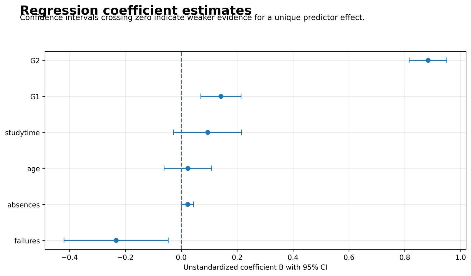
The interval plot places every original-unit slope on one horizontal scale. G2 is the dominant positive estimate, G1 is positive but much smaller, failures is negative, and absences is slightly positive. The studytime and age intervals cross zero.
G2: B = 0.883399, 95% CI [0.816222, 0.950576]. G1: B = 0.142169, 95% CI [0.070321, 0.214016]. Failures: B = −0.233156, 95% CI [−0.419571, −0.046742]. Absences: B = 0.022679, 95% CI [0.001327, 0.044031].
The plotted estimates are conditional changes in G3 for one-unit predictor increases while the other five predictors remain fixed. An interval excluding zero supplies evidence that the corresponding conditional slope differs from zero under the fitted model.
The plot prevents a common reporting error: comparing coefficient lengths without checking units and uncertainty. Original-unit Regression Coefficients are best for substantive interpretation and prediction, whereas standardized beta answers a different comparison question.
For Regression Coefficients, the interval endpoints are as important as the point estimates because they define the supported range of conditional slopes.
Python Chart 2: Standardized Beta Coefficients
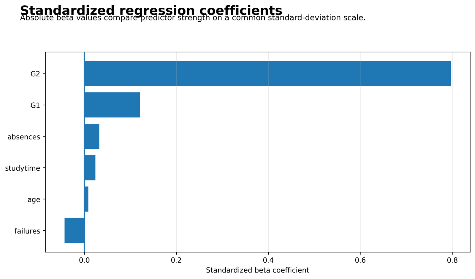
After rescaling the outcome and predictors into standard-deviation units, G2 remains far larger than every other term. G1 ranks second, while failures, absences, studytime, and age have comparatively small standardized magnitudes.
G2 β = 0.796713; G1 β = 0.120808; failures β = −0.042814; absences β = 0.032578; studytime β = 0.024284; age β = 0.008914.
A standardized beta estimates the expected standard-deviation change in G3 for a one-standard-deviation predictor increase, conditional on the other terms. It does not replace B in the original-unit prediction equation.
The ranking demonstrates that G2 supplies most of the model’s conditional grade signal. It also shows why statistical significance and standardized importance are not identical: a small beta can be significant in a large sample.
The standardized view helps compare Regression Coefficients, but original-unit B values remain necessary for prediction and substantive grade interpretation.
Python Chart 3: Regression Coefficient P-Values
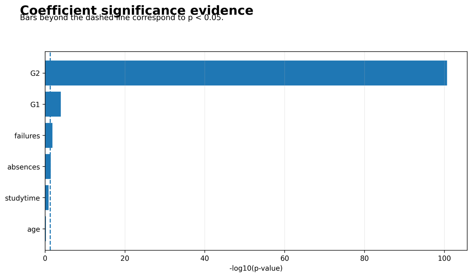
The probability-evidence chart separates the four predictors with p-values below .05 from studytime and age. G2 is visually extreme because its p-value is many orders of magnitude smaller than the others.
G2 p = 2.206 × 10⁻¹⁰¹; G1 p = 0.000113; failures p = 0.014312; absences p = 0.037398; studytime p = 0.127427; age p = 0.586762.
Each p-value evaluates a null hypothesis that one conditional slope equals zero, given the complete six-predictor equation. It does not measure effect size, practical importance, predictive value, or causality.
Reading this chart with the interval and beta plots prevents significance-only conclusions. G2 combines strong evidence with a large standardized effect, while absences combines threshold-level evidence with a very small effect.
Probability evidence should qualify Regression Coefficients rather than replace effect magnitude, interval width, and diagnostic evidence.
Python Chart 4: Observed Versus Predicted G3
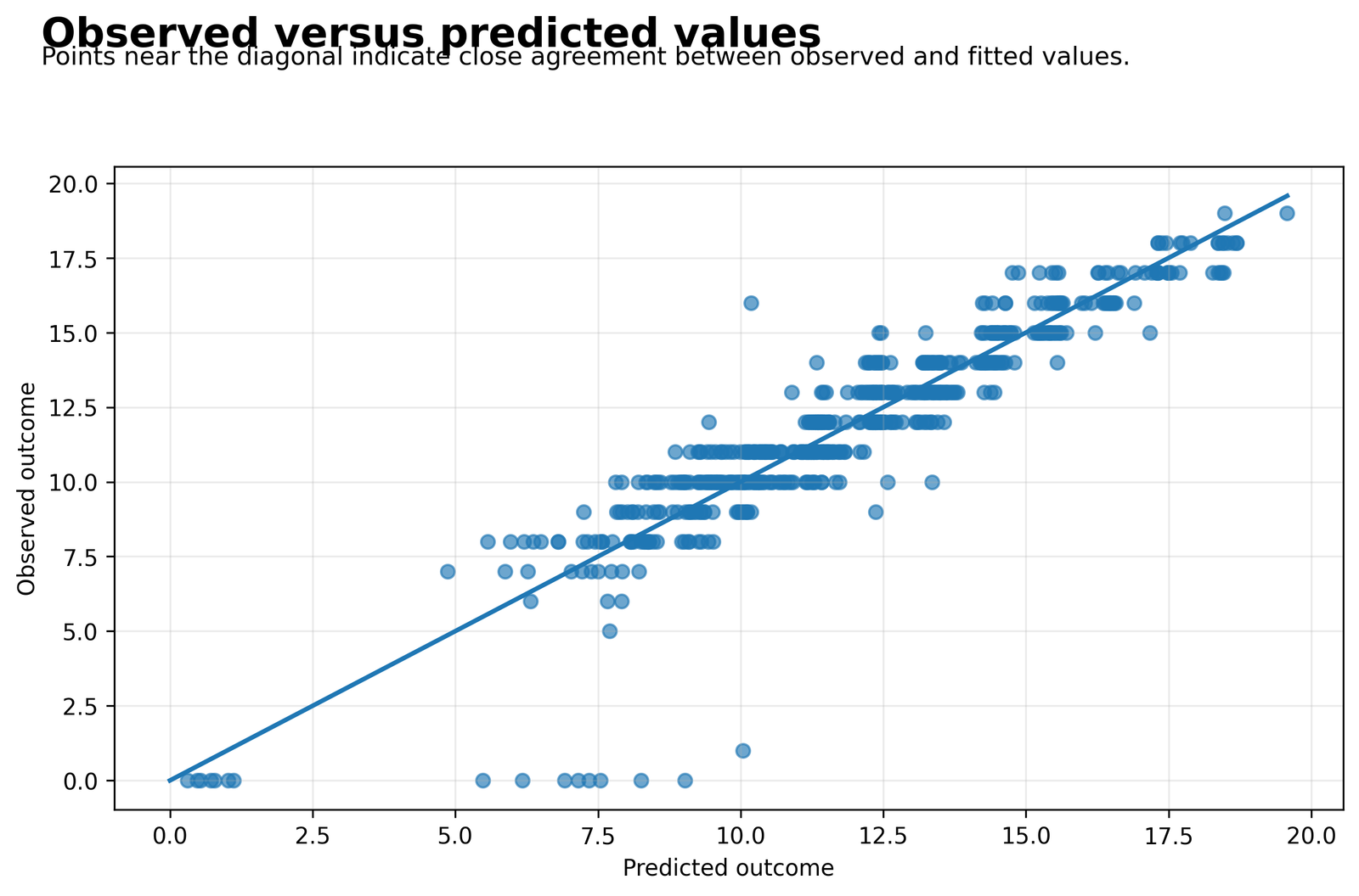
Most observations follow the identity line, with visible horizontal bands because G3 is recorded in integer grade points. The largest departures occur for several observations with very low or zero final grades that the linear equation predicts above zero.
R² = 0.850632, adjusted R² = 0.849236, RMSE = 1.254409, F(6, 642) = 609.352742, p = 3.254 × 10⁻²⁶¹.
The chart evaluates the complete equation rather than any single coefficient. Tight concentration around the identity line indicates strong in-sample reconstruction, but individual large errors remain even when overall R² is high.
Regression Coefficients should be interpreted alongside prediction error. A model can estimate a stable average slope and still perform poorly for unusual cases, especially near the lower grade boundary.
Prediction performance evaluates the full set of Regression Coefficients acting together, not the isolated importance of one predictor.
Python Chart 5: Residuals Versus Fitted Values
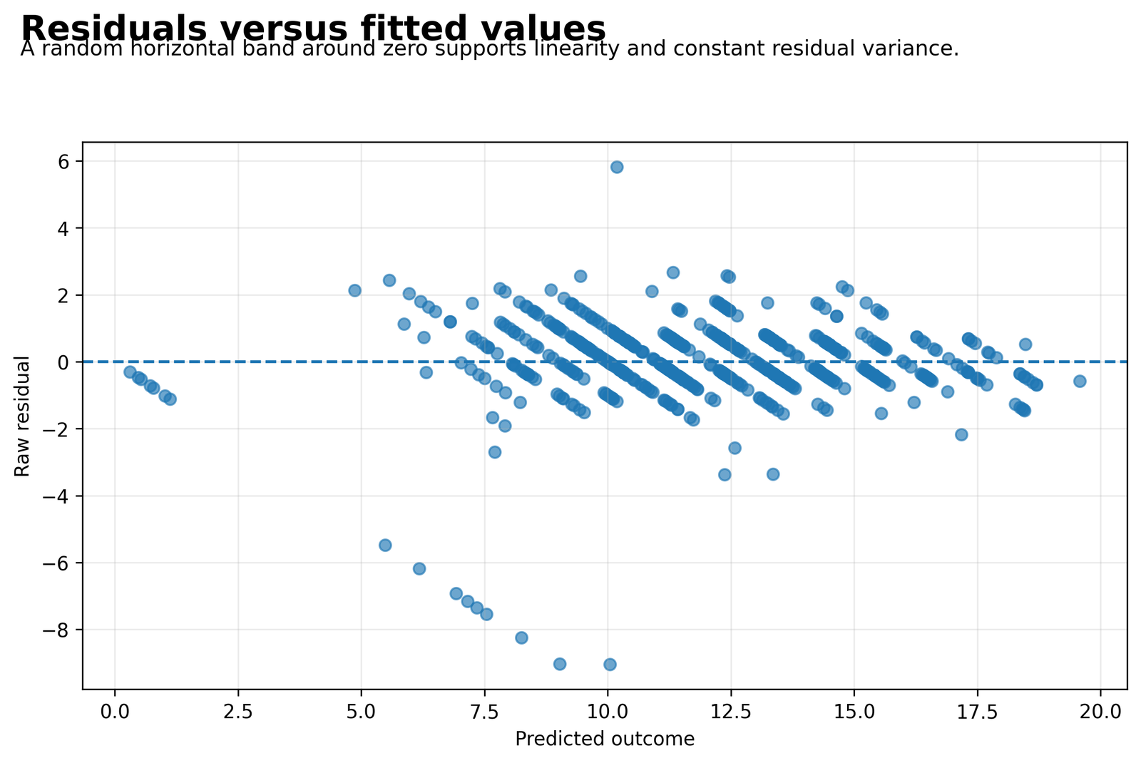
Residuals are generally centered around zero, but integer-grade banding is visible and the lower tail contains several severe negative errors. Those cases occur when predicted grades are moderate but observed G3 is zero or very low.
The most negative raw residual is about −9.044619 for case 173. Case 164 has residual −9.022936 and Cook’s distance 0.176952. The largest positive residual is 5.816804 for case 62.
Centering around zero follows from least squares with an intercept. The remaining structure is diagnostic: tail asymmetry, possible changing spread, and isolated influential cases can affect uncertainty and the stability of individual Regression Coefficients.
The plot directs the next analysis toward robust uncertainty, residual-distribution checks, and influence sensitivity rather than toward automatic deletion of every unusual observation.
Residual structure determines whether ordinary uncertainty around Regression Coefficients is sufficiently reliable for the intended report.
Python Chart 6: Residual Distribution
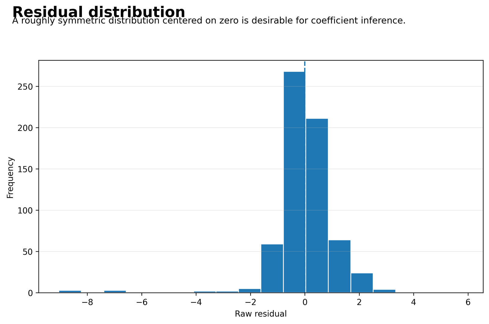
The residual histogram is concentrated near zero but has a much longer negative tail than a symmetric normal shape would produce. A smaller positive tail extends beyond five grade points.
The residual range is approximately −9.044619 to 5.816804. RMSE is 1.254409, so the most extreme residuals are several times larger than the typical model error.
Non-normal tails do not change the arithmetic definition of least-squares Regression Coefficients, but they can affect exact normal-theory inference and indicate that a small set of observations deserves influence review.
This distribution explains why coefficient tables alone are insufficient. The fitted slopes summarize the conditional mean, while the residual distribution reveals how unevenly individual cases conform to that mean.
The error distribution shows why Regression Coefficients need residual and influence evidence even when the mean model explains substantial variation.
Python Chart 7: Partial Regression Plot for G2
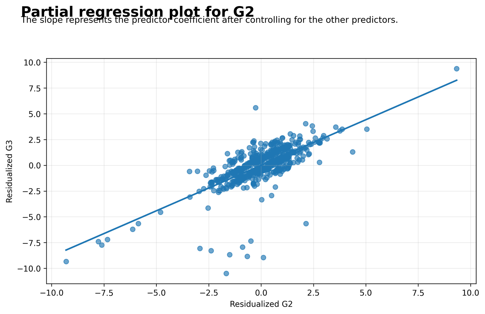
The added-variable plot remains strongly positive after the linear effects of G1, studytime, failures, absences, and age are removed from both G2 and G3. The residualized points follow a clear upward line.
G2 B = 0.883399; zero-order r = 0.918548; partial r = 0.713781; semi-partial r = 0.393882; unique R² = 0.155143.
The fitted slope in the partial regression plot equals the G2 coefficient in the complete model. The plot therefore visualizes the conditional relationship, not the larger unadjusted association between G2 and G3.
This is the clearest visual explanation of what Regression Coefficients mean in multiple regression: the G2 slope concerns the part of G2 variation not linearly explained by the other predictors.
The added-variable plot gives a direct visual interpretation of Regression Coefficients after the other predictors have been linearly controlled.
Python Chart 8: Zero-Order, Partial, and Semi-Partial Contributions
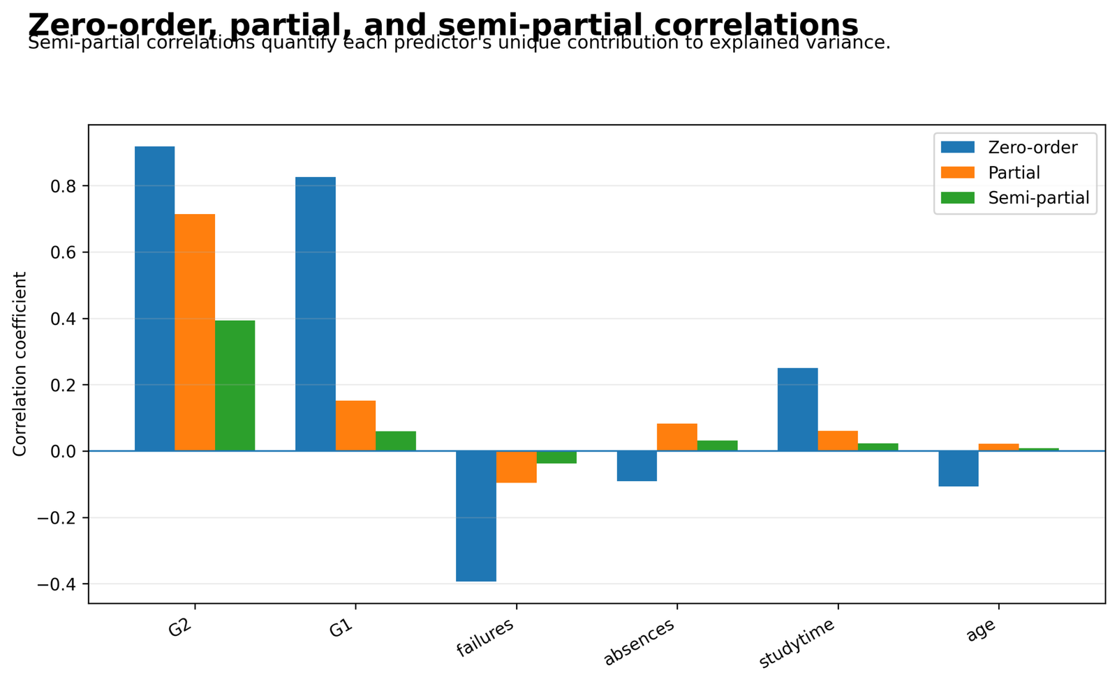
The comparison shows large reductions from simple association to adjusted and unique association for the two prior-grade variables. G2 retains a substantial unique contribution, whereas G1’s unique contribution becomes small once G2 is included.
G2: zero-order r = 0.918548, partial r = 0.713781, part r = 0.393882, unique R² = 0.155143. G1: zero-order r = 0.826387, partial r = 0.151580, part r = 0.059268, unique R² = 0.003513.
Zero-order correlation ignores the other predictors. Partial correlation removes them from both the predictor and outcome. Semi-partial correlation removes them only from the predictor, and its square equals the predictor’s unique contribution to full-model R².
The chart prevents simple correlations from being misreported as conditional effects. It also explains why G1 can have a high raw correlation with G3 but add relatively little unique fit after G2 is controlled.
The correlation comparison explains why Regression Coefficients can differ sharply from simple bivariate associations.
Four R Charts and Explanations
The R workflow uses the same formula, complete-case sample, and coefficient definitions. Agreement at full precision confirms that the Python and R results represent one model rather than similar-looking but different specifications.
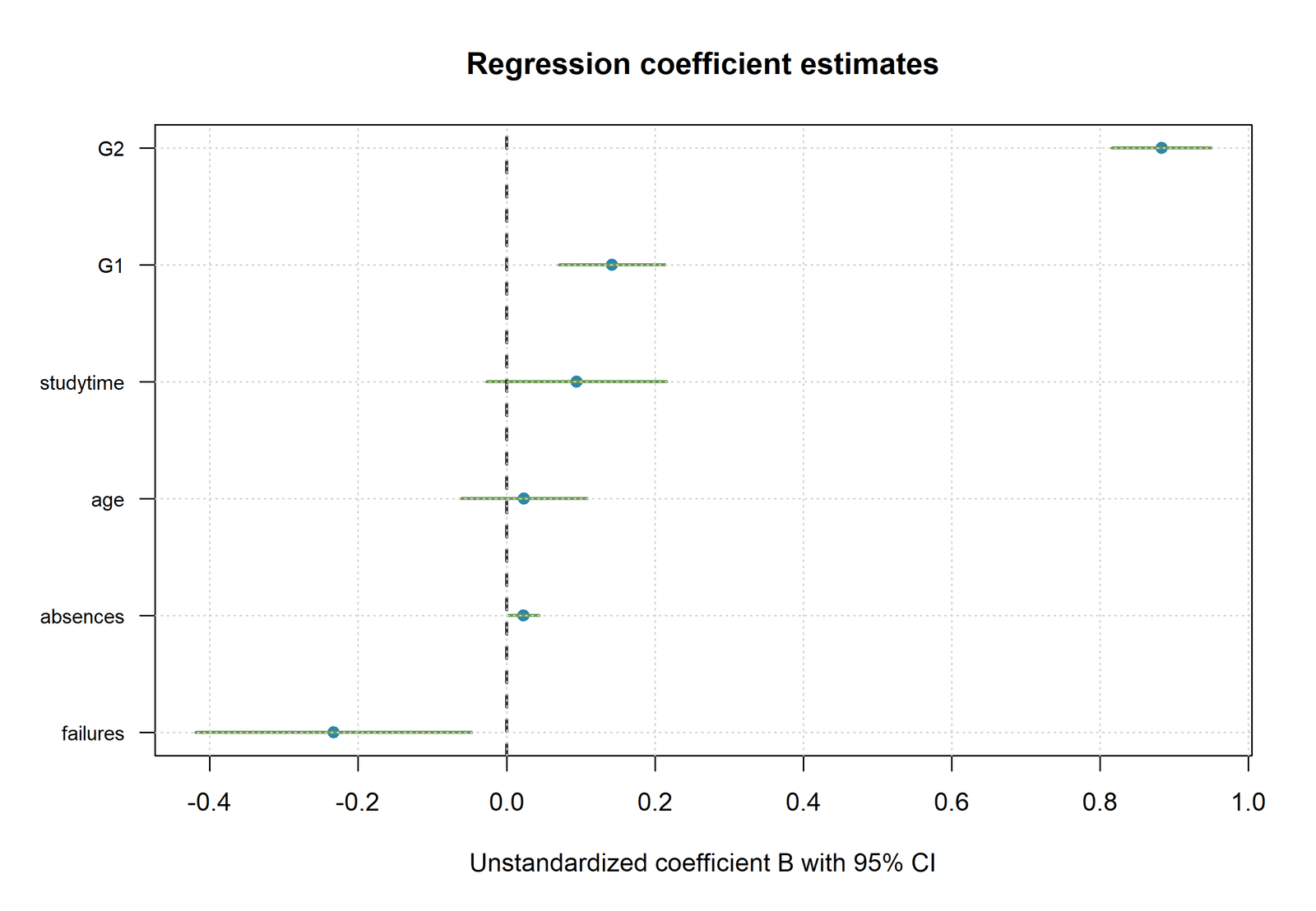
R Chart 1: Unstandardized Regression Coefficients
The R interval plot reproduces the original-unit ranking: G2 is the largest positive slope, G1 is positive, failures is negative, and absences is slightly positive. Studytime, age, and the intercept have intervals that include zero.
These Regression Coefficients remain on the original G3 scale.
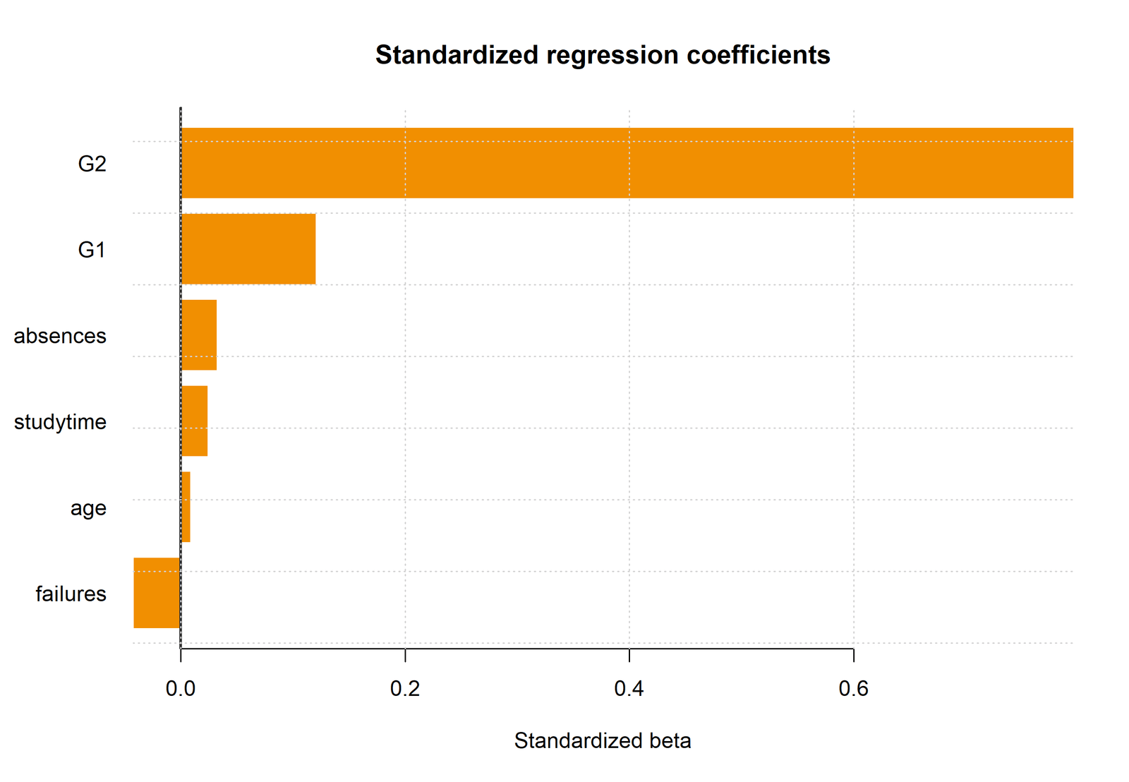
R Chart 2: Standardized Beta Ranking
The standardized R chart shows a steep drop after G2. The remaining predictors make much smaller conditional contributions on the standard-deviation scale.
These Regression Coefficients are expressed in standard-deviation units.
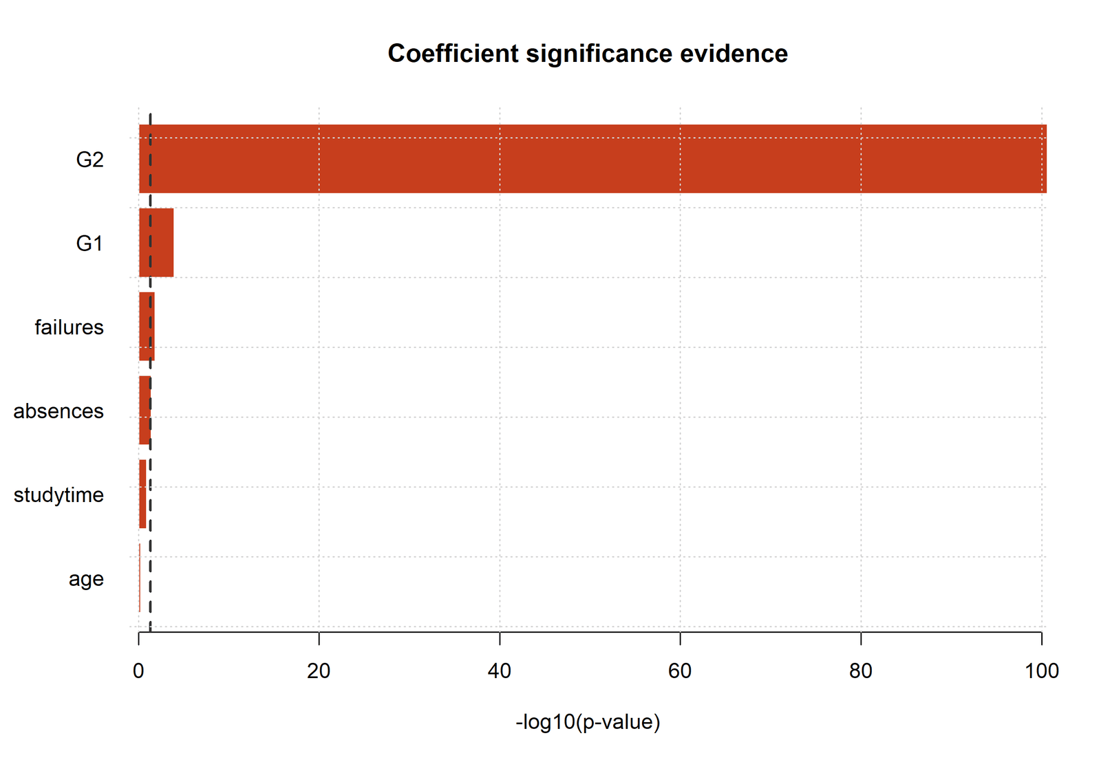
R Chart 3: P-Value Evidence
The R probability plot distinguishes G2 and G1 from the weaker terms and places failures and absences just below the .05 criterion. Studytime and age remain compatible with zero conditional slopes.
The p-value display evaluates zero-slope hypotheses for the fitted Regression Coefficients.
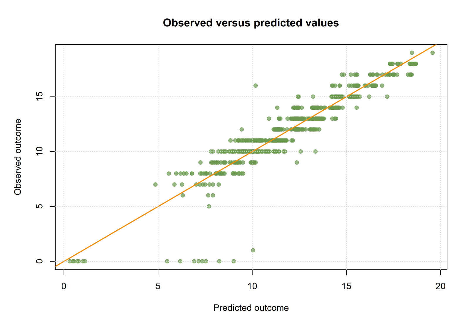
R Chart 4: Observed and Predicted Outcomes
The R observed-versus-predicted display confirms strong overall fit and the same integer-grade banding. The visibly large errors are concentrated among unusual low-outcome cases rather than spread evenly across every fitted value.
The observed-versus-predicted pattern reflects the complete set of Regression Coefficients.
How to Interpret Every Coefficient Measure
Unstandardized B
Unstandardized B is the slope used in the original prediction equation. G2 B = 0.883399 means that fitted G3 is expected to be 0.883399 points higher for a one-point G2 increase when G1, studytime, failures, absences, and age remain fixed. Because G2 and G3 use comparable grade-point units, this interpretation is direct.
Standardized beta
Standardized beta expresses both predictor and outcome changes in sample standard deviations. G2 β = 0.796713 indicates a large standardized conditional relationship. Beta is useful for ranking predictors measured in different units, but it depends on the sample’s standard deviations and is less transportable than B.
Intercept
The intercept is −0.545315. It is the fitted G3 value when G1, G2, studytime, failures, absences, and age all equal zero. That profile is not substantively representative because age and studytime cannot reasonably be zero in this sample. The intercept remains necessary to anchor the least-squares plane even when its standalone interpretation is weak.
Standard error and t statistic
The standard error describes coefficient precision under the variance model. The t statistic divides B by that standard error. A large absolute t value can result from a large slope, a precise estimate, or both. G2 combines a large slope with a small standard error, producing t = 25.822927.
P-value
The p-value evaluates the zero-slope null hypothesis within the complete equation. It does not give the probability that the null hypothesis is true, and it does not measure the chance that a reported sign will replicate. G2 has overwhelming evidence against a zero slope; the age estimate does not.
Confidence interval
A confidence interval is more informative than a binary significance label because it displays plausible magnitudes. G1’s interval [0.070321, 0.214016] supports a positive but modest conditional slope. Studytime’s interval [−0.027102, 0.216261] includes both a small negative value and a moderately positive value.
Zero-order, partial and semi-partial correlation
Zero-order correlation is the unadjusted bivariate association. Partial correlation removes the remaining predictors from both the focal predictor and outcome. Semi-partial correlation removes them only from the focal predictor; squaring it gives the unique increment to full-model R².
For G2, zero-order r = 0.918548, partial r = 0.713781, and semi-partial r = 0.393882. The differences quantify how much apparent association is shared with G1 and the other predictors.
Sign changes and suppression
Absences has zero-order r = −0.091379 but a positive coefficient B = 0.022679 and partial r = 0.082040. The sign change occurs after adjustment and may reflect shared relationships among grades, failures, age, and absence. It should be described as a suppression-like conditional pattern, not as a beneficial effect.
Unique contribution
Unique R² is the squared semi-partial correlation. G2 uniquely accounts for 0.155143 of total outcome variance beyond the other predictors. G1 uniquely accounts for 0.003513. Unique contribution is order-independent in the full simultaneous model when computed from the coefficient t statistic and full-model R².
Prediction, Residuals and Influence
How a prediction is calculated
A fitted value is constructed by multiplying each predictor by its unstandardized coefficient and adding the intercept. Standardized beta, p-values, and partial correlations are not inserted into this equation. The complete model produces one prediction for each of the 649 observations.
For case 1, the equation gives 9.877488 and the observed value is 11. The residual is therefore 11 − 9.877488 = 1.122512. A positive residual means the observed grade is higher than the model prediction.
Prediction uncertainty
A confidence interval for the mean response and a prediction interval for a new observation are different. The mean-response interval reflects uncertainty in the estimated conditional mean. A prediction interval is wider because it also includes individual residual variation. The fitted RMSE of 1.254409 summarizes typical in-sample error but is not a prediction interval.
Influential cases
Large residuals do not automatically imply high influence. Influence depends on residual magnitude and leverage together. Cook’s Distance combines those components to identify observations that may change the coefficient vector if removed.
| Case | Observed G3 | Predicted G3 | Raw Residual | Leverage | Cook’s Distance |
|---|---|---|---|---|---|
| 164 | 0 | 9.022936 | -9.022936 | 0.022859 | 0.176952 |
| 640 | 0 | 7.543323 | -7.543323 | 0.020231 | 0.108871 |
| 638 | 0 | 7.153776 | -7.153776 | 0.012981 | 0.061908 |
| 173 | 1 | 10.044619 | -9.044619 | 0.007263 | 0.054732 |
| 627 | 0 | 5.481558 | -5.481558 | 0.017505 | 0.049468 |
| 584 | 0 | 6.17939 | -6.17939 | 0.013203 | 0.047002 |
| 641 | 0 | 6.92062 | -6.92062 | 0.010225 | 0.045386 |
| 587 | 0 | 8.250282 | -8.250282 | 0.007161 | 0.044893 |
Case 164 is the strongest influence example: observed G3 = 0, predicted G3 = 9.022936, residual = −9.022936, leverage = 0.022859, and Cook’s distance = 0.176952. Case 640 also combines a severe negative residual with Cook’s distance above 0.10.
These observations should be verified, described, and examined through sensitivity refits. Automatic deletion would change the target population and could conceal a real lower-bound or mixture feature in the grade outcome. The full workbook preserves all 649 case-level predictions and diagnostics.
Assumptions and Diagnostic Consequences
Linearity and additivity
Each slope assumes that the conditional mean changes linearly with its predictor when the other terms remain fixed. Studytime’s ordered categories and the bounded grade scale make this assumption worth examining. Polynomial terms or interactions may be justified by theory, but adding them changes the meaning of the original Regression Coefficients.
Independent errors
Standard coefficient uncertainty assumes an appropriate dependence structure. If observations are clustered within schools or classes, conventional standard errors may be too small even when the coefficient point estimates are unchanged. The sampling design must therefore be considered alongside residual plots.
Homoscedasticity
Constant residual variance supports conventional OLS standard errors. The residual-versus-fitted figure shows severe low-tail observations and possible variation in spread. A formal check such as the Breusch-Pagan Test and a robust covariance estimate can determine whether the uncertainty around Regression Coefficients needs adjustment.
Residual distribution
OLS point estimates do not require the outcome itself to be normally distributed. Normal residual assumptions concern exact small-sample t and F inference. The long negative residual tail suggests that a Q-Q Plot Normality Check and robust sensitivity analysis should accompany conventional inference.
Multicollinearity
G1 and G2 have VIF values around 4.1. Shared information inflates their standard errors and makes each coefficient a conditional effect beyond the other grade. See Variance Inflation Factor, Tolerance Statistic, and Multicollinearity Check for complementary diagnostics.
Influence and data quality
The largest negative residuals occur among observations with zero or very low G3. These may be valid outcomes, structural zeros, coding issues, or cases generated by a different process. Outlier Detection and Influence Diagnostics should separate data verification from model sensitivity.
Causal interpretation
Even perfectly diagnosed Regression Coefficients remain conditional associations unless the design identifies causal effects. Prior grades, failures, and absences can be related to unmeasured ability, health, motivation, school conditions, and selection. The positive absence coefficient therefore cannot justify an intervention claim.
Regression Coefficients remain interpretable only when the stated functional form and uncertainty method are made explicit.
Regression Coefficients in Python, R, SPSS and Excel
Python
- Fit OLS with
statsmodels.api.OLS. - Read B, standard error, t, p, and confidence intervals from the fitted result.
- Calculate standardized beta from sample standard deviations.
- Use influence methods for leverage, studentized residuals, and Cook’s distance.
Python reproduces the Regression Coefficients and influence measures at full precision.
R
- Fit the equation with
lm(). - Use
summary()andconfint()for coefficient inference. - Calculate beta, partial, and semi-partial measures using the same complete cases.
- Use
influence.measures(),hatvalues(), andcooks.distance().
R estimates the same Regression Coefficients when the formula and complete cases match.
SPSS
- Read B from the Unstandardized Coefficients column.
- Read standardized beta from the Beta column.
- Request confidence intervals, tolerance, VIF, residuals, leverage, and Cook’s distance.
- Keep the predictor block identical to the Python and R model.
SPSS separates unstandardized and standardized Regression Coefficients in the Coefficients table.
Excel
- Replay predictions with exact B values and cell references.
- Calculate residuals as observed minus predicted.
- Calculate t as B divided by standard error and intervals with the t distribution.
- Use the workbook for auditing rather than replacing matrix-based software diagnostics.
Excel is most useful for auditing Regression Coefficients and replaying fitted values.
Apparent software disagreement usually comes from different missing-data rules, predictor coding, intercept handling, standard-deviation conventions, or rounding. Compare the full formula and analysis sample before comparing printed Regression Coefficients.
Regression Coefficients Code
Each code block fits or reconstructs the same six-predictor model. Replace variable or cell references only when the research specification changes.
Python: fit, intervals, standardized beta and influence
import statsmodels.api as sm

predictors = ["G1", "G2", "studytime", "failures", "absences", "age"]
d = df[["G3"] + predictors].dropna()

X = sm.add_constant(d[predictors], has_constant="add")
fit = sm.OLS(d["G3"], X).fit()

print(fit.summary())
print(fit.conf_int(alpha=0.05))

beta = fit.params[predictors] * d[predictors].std(ddof=1) / d["G3"].std(ddof=1)
print(beta.sort_values(key=abs, ascending=False))

influence = fit.get_influence()
diagnostics = d.assign(
    predicted=fit.fittedvalues,
    residual=fit.resid,
    leverage=influence.hat_matrix_diag,
    cooks_distance=influence.cooks_distance[0]
)
R: lm coefficients, confidence intervals and diagnostics
predictors <- c("G1","G2","studytime","failures","absences","age")
d <- na.omit(dataset[c("G3", predictors)])

fit <- lm(G3 ~ G1 + G2 + studytime + failures + absences + age, data=d)

summary(fit)
confint(fit, level=.95)

beta <- coef(fit)[predictors] *
        sapply(d[predictors], sd) / sd(d$G3)
sort(beta, decreasing=TRUE)

diagnostics <- transform(
  d,
  predicted=fitted(fit),
  residual=residuals(fit),
  leverage=hatvalues(fit),
  cooks_distance=cooks.distance(fit)
)
SPSS: coefficient and collinearity output
REGRESSION
 /DEPENDENT G3
 /METHOD=ENTER G1 G2 studytime failures absences age
 /STATISTICS COEFF OUTS R ANOVA COLLIN TOL CI(95)
 /SAVE PRED RESID SRESID COOK LEVER.

* Standardized Beta is shown in the Beta column.
* Use unstandardized B values for the original-unit equation.
* Verify that N = 649 and residual df = 642.
Excel: prediction and coefficient formulas
Prediction:
=$B$2+$B$3*B2+$B$4*C2+$B$5*D2+$B$6*E2+$B$7*F2+$B$8*G2

Residual:
=Observed_G3-Predicted_G3

t statistic:
=Coefficient_B/Standard_Error

95% lower:
=Coefficient_B-T.INV.2T(0.05,642)*Standard_Error

95% upper:
=Coefficient_B+T.INV.2T(0.05,642)*Standard_Error

Standardized beta:
=Coefficient_B*STDEV.S(Predictor_Range)/STDEV.S(Outcome_Range)
Advanced Regression Coefficients Topics
1. What a Regression Coefficient Represents
A regression coefficient is a parameter of a specified conditional mean function. It belongs to the equation, coding, analysis sample, and predictor set used to estimate it. Changing any of those elements can change the number and its meaning.
2. Unstandardized B
Unstandardized B preserves the original predictor and outcome units. It is the correct coefficient for direct prediction and for statements such as expected grade-point change per additional prior-grade point.
3. Standardized Beta
Standardized beta rescales B using sample standard deviations. It is useful for ranking predictors within one sample, but it changes when the sample variability changes and should not be treated as a universal effect size.
4. The Intercept
The intercept is the fitted outcome at zero on every predictor. It should be retained unless the model is intentionally constrained through the origin. Centering predictors can make the intercept more meaningful without altering fitted values.
5. Standard Error
The Standard Error measures coefficient uncertainty under the variance and dependence assumptions. A large standard error can arise from limited information, high residual variance, restricted predictor range, or multicollinearity.
6. t Statistic
The t statistic is B divided by its standard error. It measures how many estimated standard errors the coefficient lies from zero, not how many outcome units the predictor changes.
7. P-Value
The P-Value addresses a null hypothesis about one conditional slope. It should be read with the estimate, interval, model specification, and multiplicity context rather than used as a standalone importance score.
8. Confidence Interval
A Confidence Interval communicates direction and precision. Wide intervals indicate that materially different coefficient values remain compatible with the data even when the point estimate appears meaningful.
9. Zero-Order Correlation
A zero-order correlation is the unadjusted relationship between one predictor and the outcome. It is not a multiple-regression coefficient because it does not hold the other predictors constant.
10. Partial Correlation
Partial Correlation removes the remaining predictors from both the focal predictor and the outcome. It quantifies the adjusted association among the residualized variables.
11. Semi-Partial Correlation
Semi-Partial Correlation removes the remaining predictors only from the focal predictor. Its square is the predictor’s unique contribution to the complete model’s R².
12. Unique R-Squared Contribution
Unique R² answers how much full-model explained variation would be lost when one predictor is removed while the others remain. It is often more informative for incremental value than the standardized beta alone.
13. Shared Predictor Information
When predictors overlap strongly, their simple correlations can be large while unique contributions are small. G1 and G2 illustrate this distinction because both contain prior-grade information.
14. Suppression and Sign Reversal
A coefficient can have a different sign from its zero-order correlation after control variables are included. Such a reversal should be investigated through correlations, coding, theory, and sensitivity models rather than interpreted causally.
15. Multicollinearity
Multicollinearity mainly affects coefficient precision and stability. It does not automatically make predictions poor, and removing a theoretically important predictor solely to reduce VIF can create omitted-variable bias.
16. Reference Categories
For a categorical predictor, each indicator coefficient compares one category with the omitted reference category. Changing the reference category changes individual coefficients but not the fitted values or overall model fit.
17. Interaction Terms
With an interaction, the coefficient of one predictor is its effect when the interacting variable equals zero. Marginal effects or predicted values across meaningful moderator levels are usually clearer than interpreting one coefficient in isolation.
18. Polynomial Terms
When X and X² are entered, the linear coefficient is not a constant slope across the predictor range. The instantaneous slope changes with X, so plots and derivatives are needed for interpretation.
19. Centering Predictors
Mean centering changes the intercept and lower-order terms in interaction or polynomial models but does not change fitted values. Centering can make zero a meaningful reference point and reduce nonessential collinearity.
20. Robust Standard Errors
Heteroskedasticity-robust covariance changes standard errors, t statistics, p-values, and intervals without changing OLS B values. Report both the estimator and the uncertainty method.
21. Omitted-Variable Bias
A coefficient can be biased when an omitted variable affects the outcome and is related to an included predictor. Statistical significance and high R² do not rule out this problem.
22. Measurement Error
Random measurement error in a predictor commonly attenuates its coefficient toward zero and can redistribute association among correlated predictors. Reliability therefore matters for coefficient interpretation.
23. Influential Observations
Cook’s Distance and related diagnostics identify cases capable of changing Regression Coefficients. Influence should lead to verification and sensitivity analysis, not automatic exclusion.
24. Prediction Versus Explanation
A coefficient can be unstable while predictions remain accurate because correlated predictors compensate for one another. Conversely, a stable coefficient does not guarantee strong out-of-sample prediction.
25. Comparing Coefficients Across Models
A coefficient can change when controls are added because the estimand changes. Comparisons across models should describe the differing conditioning sets rather than labeling movement as inconsistency.
26. Reproducible Reporting
Reproducible coefficient reporting records the formula, sample, coding, software, estimator, uncertainty method, precision, and diagnostic decisions. Full-precision files should be preserved even when the article displays rounded values.
APA-Style Reporting
APA reporting should present Regression Coefficients with their units, uncertainty, conditioning set, and diagnostic qualifications.
G2 was the strongest predictor, B = 0.883, SE = 0.034, β = .797, t(642) = 25.82, p < .001, 95% CI [0.816, 0.951]. G1 also had a positive conditional association, B = 0.142, SE = 0.037, β = .121, t(642) = 3.89, p < .001, 95% CI [0.070, 0.214].
Failures was negatively associated with G3, B = −0.233, SE = 0.095, β = −.043, t(642) = −2.46, p = .014, 95% CI [−0.420, −0.047]. Absences had a small positive conditional coefficient, B = 0.023, SE = 0.011, β = .033, t(642) = 2.09, p = .037, 95% CI [0.001, 0.044].
Studytime, B = 0.095, p = .127, and age, B = 0.024, p = .587, did not have intervals excluding zero. G2 uniquely accounted for 15.51% of total G3 variance beyond the other predictors, whereas G1 uniquely accounted for 0.35%.
Residual and influence diagnostics identified several observations with severe negative residuals; case 164 had Cook’s distance = 0.177. The reported Regression Coefficients should therefore be accompanied by influence sensitivity and robust uncertainty checks.
Publication Checklist
The checklist keeps Regression Coefficients connected to the exact model rather than to a generic significance rule.
Report
- The exact outcome and predictor formula
- Sample size and missing-data rule
- Unstandardized B and original units
- Standard error, t, p, and confidence interval
- Standardized beta when comparing scales
- Reference category for categorical predictors
- R², adjusted R², RMSE, and overall F test
- Multicollinearity, residual, and influence evidence
- Robust or sensitivity results when diagnostics require them
Avoid
- Calling a coefficient a causal effect without identification
- Using beta in the raw prediction equation
- Reporting p-values without magnitude and uncertainty
- Comparing B values measured in incompatible units
- Calling a non-significant coefficient exactly zero
- Deleting every case with a diagnostic flag
- Interpreting the intercept outside the observed predictor range
- Comparing coefficients from different models as identical estimands
- Ignoring sign reversals between zero-order and adjusted results
Connect Regression Coefficients with Effect Size, Adjusted R Squared, Regression Assumptions, and Residual Analysis rather than treating the coefficient table as the entire analysis.
Downloads
The downloadable files preserve the full-precision Regression Coefficients used throughout this guide.
Regression Coefficients R ReportIndependent R estimation and validation charts
Regression Coefficients SPSS OutputB, Beta, t, significance, confidence intervals and collinearity output
Regression Coefficients Worked ExcelEquation replay, coefficient calculations and 649 case-level checks
Frequently Asked Questions
What are Regression Coefficients?
Regression Coefficients are parameters that describe how the fitted conditional mean changes with predictors. In multiple linear regression, each slope holds the remaining predictors constant.
What is the difference between B and beta?
B uses original units and builds the prediction equation. Standardized beta uses standard-deviation units and is mainly used to compare conditional magnitudes within one model.
How do I interpret a positive coefficient?
A positive coefficient means fitted outcome values increase as the predictor increases, conditional on the other model terms. It does not automatically imply a beneficial or causal effect.
How do I interpret a negative coefficient?
A negative coefficient means fitted outcome values decrease as the predictor increases while the other listed predictors stay fixed. The scale and coding must be stated.
What does the intercept mean?
The intercept is the fitted outcome when every predictor equals zero. It may be mathematically necessary even when an all-zero predictor profile is not substantively meaningful.
How is the t statistic calculated?
The t statistic equals B divided by its standard error. It evaluates the zero-slope null hypothesis using the residual degrees of freedom.
What does a coefficient p-value mean?
It measures how incompatible the observed t statistic is with a zero conditional slope under the fitted model. It is not the probability that the null hypothesis is true.
Why should I report a confidence interval?
A confidence interval shows the direction, precision, and range of plausible coefficient magnitudes. It communicates more than a significant or non-significant label.
Why is G1 strongly correlated with G3 but weak uniquely?
G1 shares substantial information with G2. After G2 and the other predictors are controlled, G1’s semi-partial correlation is only 0.059268 and unique R² is 0.003513.
Why is the absences coefficient positive?
The sign changes after adjustment because absences shares relationships with grades, failures, age, and other predictors. The small positive coefficient is conditional and should not be interpreted causally.
Can a significant coefficient be unimportant?
Yes. Large samples can make small slopes statistically detectable. Absences has p = .037 but standardized beta is only .0326.
Can a non-significant predictor remain in the model?
Yes, when theory, design, confounding control, hierarchy, or prediction goals justify it. Deletion based only on p-values can change the estimand and bias other coefficients.
How does multicollinearity affect coefficients?
It increases uncertainty and can make individual slopes sensitive to small data or specification changes. It does not necessarily damage overall predictions.
How are predictions calculated?
Multiply each predictor by its unstandardized B, add the products, and add the intercept. Do not use standardized beta or p-values in the raw equation.
Why can software show slightly different values?
Differences usually arise from missing-data handling, coding, standard-deviation conventions, robust covariance choices, or printed rounding. Identical data and formulas should agree closely.
How should Regression Coefficients be reported?
Report B, standard error, t, p, confidence interval, units, conditioning set, sample size, model fit, and diagnostics. Add standardized or unique-contribution measures when they answer the research question.
Regression Coefficients Conclusion
The six-predictor model shows how one coefficient table contains several layers of meaning. G2 has the largest original-unit slope, standardized beta, partial correlation, and unique contribution. G1 remains positive but contributes much less unique variation after the shared prior-grade information in G2 is controlled.
Failures has a negative conditional coefficient, while absences has a small positive coefficient that reverses its zero-order sign. Studytime and age have intervals spanning zero. These findings describe the fitted conditional mean and should not be converted into causal claims.
Strong model fit does not eliminate case-level problems. Several observations with zero or very low G3 produce severe negative residuals and meaningful Cook’s distances. The most defensible report preserves the original Regression Coefficients, adds influence sensitivity, and evaluates robust uncertainty.
Regression Coefficients become most informative when the article preserves both the fitted equation and the evidence that qualifies it.

